
Microfacet Distribution Function:
To Change or Not to Change, That Is the Question
Dariusz Sawicki
a
Warsaw University of Technology, Institute of Theory of Electrical Engineering,
Measurements and Information Systems, Warsaw, Poland
Keywords: Microfacet Distribution Function, MDF, Slope Distribution, Normal Distribution Function, Reflectance
Models, BRDF.
Abstract: In computer graphics and multimedia, bidirectional reflectance distribution function (BRDF) is commonly
used for modeling the reflection and refraction of light. In this study, one of the important components of the
reflectance models, namely, the microfacet distribution function (MDF) has been considered. The analytical
MDFs allow only approximating the real distribution of the surface. Modern graphic software gives the
opportunity to select the MDF that fits the real reflection in the best way. The question arises: can we really
replace one MDF with another in this situation? And if it is possible, how to convert parameters from one
function to the other. The problem is topical, important and practical—for all users of graphic software. In
this article, various examples of MDF have been discussed. After RMSE analysis the mathematical
dependencies that allow for the exchange of one MDF with the other have been proposed. In this study,
consequences of applying different MDFs have been also discussed and comparison of the visual effect has
been presented.
1 INTRODUCTION
For many years, one of the most difficult tasks in
computer graphics is modeling the reflection of light
in the most consistent and realistic manner. The
behavior of the light—object interaction depends on
the material and surface properties of the object. Such
phenomena are described in computer graphics by the
BRDF (Dorsey et al., 2008). One of the important
components of the reflectance models is the
microfacet distribution function (MDF) (Hall, 1989).
MDF is used in the category of BRDF whose form
arises from the assumption that the surface has a
microstructural character. Many interesting
comparative studies about BRDF have been
published (Hall, 1989, Kurt and Edwards, 2009, Ngan
et al., 2004, Ngan et al., 2005, Rusinkiewicz, 1997,
Schlick, 1994b). It seems that the topic is closed;
however, recent publications show that the problem
is still valid and worthy of further research. The
anisotropic BRDF has been described in 1992 (Ward,
1992). In 2010, a new anisotropic BRDF was
proposed with a discussion on the MDF (Kurt et al.,
a
https://orcid.org/0000-0003-3990-0121
2010). In 2015, a new iridescent rendering method
was proposed (Kang et al., 2015), based on
modification (multi-peak) of anisotropic MDF.
However, this method (and MDF) was designed to
special kind of surfaces/reflection (different
wavelengths reflection, diffraction effects) and
cannot be compared to general purpose MDFs.
Modern graphic programs allow modeling the
reflective properties of the material’s surface in the
best way with the appropriate BRDF. Advanced
graphic programs allow not only changing BRDF but
also modifying their components. It allows selecting
MDF to the expectations related to the real reflection.
On the other hand, it is known research on MDF
shape to match the analytical character BRDF to real
measurements of reflection. The authors of the work
(Bagher et al., 2012) adjusted the form of MDF for
Cook-Torrance BRDF, considering real examples of
light reflection. The question arises: can we really
replace one MDF with the other in this situation and
what will be the consequences. There are many
publications describing various BRDFs.
Unfortunately, comparative analyses of MDF have
Sawicki, D.
Microfacet Distribution Function: To Change or Not to Change, That Is the Question.
DOI: 10.5220/0010252702090220
In Proceedings of the 16th International Joint Conference on Computer Vision, Imaging and Computer Graphics Theory and Applications (VISIGRAPP 2021) - Volume 1: GRAPP, pages
209-220
ISBN: 978-989-758-488-6
Copyright
c
2021 by SCITEPRESS – Science and Technology Publications, Lda. All rights reserved
209

been rarely reported in literature. There is only one
book in which the properties of MDF are widely
considered and several MDFs have been compared
(Hall, 1989). The visual comparison on some MDFs
can be found in publications from last years (Heitz
2014, Ribardière et al., 2019).
This article is aimed at analyzing the properties of
various analytical MDFs. On the one hand, this
analysis will allow for the conversion of the
parameters value between MDF to get the most
similar graphics. On the other hand, the analysis will
allow to reveal the differences between MDF and will
show the consequences of such a change. Today, a big
challenge in practical applications is the attempt of
fitting the MDF model to the real, measured
(captured) reflection conditions of the surface
(Bringier et al., 2020). And for this, knowledge of the
properties of various known MDFs is needed.
2 MATERIAL AND METHODS
2.1 BRDF
A description of the BRDF itself does not seem to be
necessary, because this function is known to all those
dealing with computer graphics. However, a detailed
description of basic characteristics and parameters is
necessary for consistency with the description later in
this article.
The BRDF 𝑓𝐿
⃗
,𝑉
⃗
, introduced by Nicodemus
(Nicodemus, 1970, Nicodemus et al., 1977), can be
defined in the form of a simple equation—the
quotient of 𝑑𝐿(𝑉
⃗
) and 𝑑𝐸(𝐿
⃗
) (the outgoing radiance
and the incoming irradiance, respectively).
Many different models of reflection exist because
there is no universal mathematical description of light
reflection for any surface and material. The best
effects are obtained using the reflection model created
based on the appropriate physical theory regarding
the smoothness (roughness) of the surface (Pharr et
al., 2016). In this case, the BRDF’s description has
the general form (1) with a set of specular
components:
𝑓
𝐿
⃗
,𝑉
⃗
=
𝑘∙𝐹
(
𝜃
)
∙𝐺∙𝐷
𝑀
(1)
where F(
θ
) is the Fresnel factor of reflectivity
(depends on the incidence angle
θ
); G is the geometric
attenuation; D represents the MDF; M is the factor
that describes the angle reflection properties,
especially for surface of materials with good
properties of specular reflection (e.g. metals)
(Neumann et al., 1999); and k is the factor which
allows fulfilling the energy conservation law.
There are many well-known BRDFs with form
similar to (1): BRDFs, Cook-Torrance (Cook and
Torrance, 1981), He (He, 1994, He et al., 1991, He et
al., 1992), Embrechts (Embrechts, 1995, Embrechts,
1999), and Ashikhmin-Shirley (Ashikhmin and
Shirley, 2000). A short analysis of the role of specular
component from (1) can be found in (Mac Manus,
2009).
The crucial element of the discussed BRDF forms
is the MDF represented as D in equation (1). Several
different forms or approximations of the distribution
function exist. It is worth analyzing the properties;
similarities, and differences of these functions and
their influence on the defined picture and the
computational process.
2.2 MDF: Overview and Properties
To be able to replace one MDF with the other, it is
necessary to analyze their properties. The MDF
characterizes smoothness/roughness of the material’s
surface, and it determines the directional relation of
reflection. The function is also called slope
distribution (Schlick, 1994b) or roughness function
(Hall, 1989). Sometimes it exists as normal
distribution function (Akenine-Möller et al., 2008,
Dong et al., 2015, Ribardière et al., 2019) as well. The
first analysis of different MDFs can be found in
Blinn’s famous study (Blinn, 1977). The book (Hall,
1989) contains more information about MDF, some
basic comparison of the functions, and C-source code
examples. The MDF was also analyzed as a BRDF
component in (Schlick, 1994c). It is noteworthy that
the MDF can also be used in the description of the
refraction phenomenon (Walter et al., 2007).
The MDF is most often defined as a function of
the
β
angle between normal vector 𝑁
⃗
and 𝐻
⃗
vector.
Where 𝐻
⃗
vector bisects the angle between vectors to
observer and to source of light. The energy
conservation law requires that D meets the
normalization condition. There exist many
descriptions of MDF normalization (Akenine-Möller
et al., 2008, Pharr et al., 2016, Schlick, 1994c)
depending on the assumed BRDF formula. For
isotropic behavior and for MDF in formula dependent
on the
β
angle, the normalization equation (Schlick,
1994c) is as follows (2):
𝐷
(
𝛽
)
∙2∙𝑐𝑜𝑠𝛽∙𝑠𝑖𝑛𝛽∙𝑑𝛽
⁄
=1
(2)
GRAPP 2021 - 16th International Conference on Computer Graphics Theory and Applications
210

The authors describing MDFs did not always care
about meeting the normalization condition (2). In
such a case, the calculations do not fulfill energy
conservation law, and it was corrected within an
independent study later. This was the case of the
Phong reflection model—the expression considers an
alteration (Lafortune and Willems, 1994, Lewis,
1994) to the original Phong formula.
In this study, the unit form (marked as 𝐷
) is
considered. This facilitates comparison of different
functions of distribution. Unit form means 𝐷
=
𝐷/𝑚𝑎𝑥(𝐷), in most cases of distribution function,
the maximum value occurs for
β=
0. It means 𝐷
=
𝐷/𝐷(0) (Table 1).
The MDF, as the special defined function, has
been introduced in a book (Beckmann and
Spizzichino, 1963). The authors have provided a
theoretical analysis of the electromagnetic waves’
reflection from random rough surface and proposed a
statistical description of the surface roughness. They
assumed the polyhedral character of the surface
roughness. Authors justified the need to use the MDF
and provided a comprehensive analysis of the
proposed Beckmann formula (Table 1) as a function
of the
β
angle. m
B
∈
(0,1) is the parameter that
characterizes the surface smoothness and
reflectivity—the smaller the value is, the closer the
reflection is to the perfect directional one.
The first (historically) microfacet distribution
function used in the BRDF was the Gauss expression
(Torrance and Sparrow, 1967). In this formula
(Table 1) C
TS
describes smoothness/roughness of the
material—it determines the distribution of the faces’
slope about the mean-surface plane in a polygonal
Table 1: Discussed microfacet distribution functions in normalized and unit form.
Author /used by/ Normalized form Unit form
Beckmann Spizzichino
(Beckmann and Spizzichino,
1963)
/Cook Torrance (Cook and
Torrance, 1981)/
/Embrechts (Embrechts, 1995,
Embrechts, 1999
)
/
𝐷
=
1
𝜋∙𝑚
∙𝑐𝑜𝑠
𝛽
∙𝑒
𝐷
=
1
𝑐𝑜𝑠
𝛽
∙𝑒
Gauss
/Torrance Sparrow (Torrance and
Sparrow, 1967)/
𝐷
=
2 ∙ 𝑙𝑛𝑐𝑜𝑠𝛽
−𝑙𝑛2
2 ∙ 𝜋∙ 𝑙𝑛𝑐𝑜𝑠𝛽
∙𝑒
and
𝐶
=1/𝑚
, 𝛽
=𝑚
∙
𝑙𝑛(2)
𝐷
=𝑒
Trowbridge Reitz (Trowbridge
and Reitz, 1975)
/GGX model (Burley, 2012)
/
𝐷
=
1
𝜋
𝐶
𝑐𝑜𝑠
𝛽∙
(
𝐶
−1
)
+1
𝐷
=
𝐶
𝑐𝑜𝑠
𝛽∙
(
𝐶
−1
)
+1
GTR model
(Burley, 2012)
𝐷
=
1
𝜋
𝐶
(
𝑐𝑜𝑠
𝛽∙
(
𝐶
−1
)
+1
)
Practically in applications 1.5<γ<3,
for γ>10
D
GT
R
is very similar to analysis
in
(
Ribardière et al., 2017
)
𝐷
=
𝐶
𝑐𝑜𝑠
𝛽∙
(
𝐶
−1
)
+1
Blinn/Phong (Blinn, 1977,
Lewis, 1994, Phong, 1975),
/Strauss (Strauss, 1990)/
Anisotropic version:
Ashikhmin-Shirley (Ashikhmin
and Shirley, 2000)/modified
in (Pharr et al., 2016)
𝐷
=
𝑁+2
2𝜋
𝑐𝑜𝑠
𝛽∙
𝐷
=
(𝑁
+2)∙(𝑁
+2)
2𝜋
𝑐𝑜𝑠
𝛽∙
where 𝑝=𝑁
∙𝑐𝑜𝑠
+𝑁
∙𝑠𝑖𝑛
φ
– the angle of anisotropy
𝐷
=𝑐𝑜𝑠
𝛽
Schlick (Schlick, 1994c)
𝐷
=
𝑚
∙𝑥
𝜋 ∙ 𝑐𝑜𝑠𝛽∙(𝑚
∙𝑥
−𝑥
+𝑚
)
where 𝑥=𝑐𝑜𝑠𝛽+𝑚
−1
𝐷
=
𝑚
∙𝑥
𝑐𝑜𝑠𝛽∙ (𝑚
∙𝑥
−𝑥
+𝑚
)
where 𝑥=𝑐𝑜𝑠𝛽+𝑚
−1
Sawicki (Sawicki,2006)
𝐷
=
96∙(3+𝑁
)∙𝑐𝑜𝑠𝛽
𝜋∙((1−𝑁
)∙𝑐𝑜𝑠𝛽+𝑁
+3)
𝐷
=
256 ∙ 𝑐𝑜𝑠𝛽
((1 − 𝑁
)∙𝑐𝑜𝑠𝛽+𝑁
+3)
Microfacet Distribution Function: To Change or Not to Change, That Is the Question
211

model of the surface. According to the similarity
between the Gauss and Beckmann formulas, the C
TS
parameter in the Gauss formula is expressed as 1/m
G
(Table 1).
Blinn (Blinn, 1977) discussed the usage of Gauss
distribution in a similar form. MDF in the form of the
Gauss function also appears in contemporary
literature (Ashikhmin et al., 2000). Cook and
Torrance in their model of BRDF used the Beckmann
distribution function. There is also a documented
possibility (Lengyel, 2002) of adding anisotropic
feature of reflection into Beckmann distribution by
modifying this equation. Schlick (Schlick, 1994c)
proposed the rational approximation (Table 1) as the
answer to the computational complexity of
Beckmann distribution. The apparent computational
simplicity of the Shlick equation (Table 1) is
connected with an additional condition: the
distribution is defined only for cos
β∈
[1 – m
B
, 1]. An
attempt to use this formula for a full range of the
β
angle leads to major errors (Sawicki, 2006). In some
cases, it makes the calculations significantly difficult.
Schlick also proposed (Schlick, 1994b) another MDF
equation that approximated the Beckmann
distribution. However, a significant difference of
shape to original distribution resulted in such
proposition never being used. Therefore, in this study,
the term “Schlick distribution” denotes the original
equation from (Schlick, 1994c).
The Torrance-Sparrow and Cook-Torrance
models and Schlick approximation were developed
with the assumption of the polygonal character of the
surface smoothness (roughness). In this way, the
MDF specifies the distribution of the microfacets of
the material. The distribution proposed by in
(Trowbridge and Reitz, 1975) (Table 1), is the next
solution that is worth taking into consideration. It also
represents a physically well-grounded model but with
a different assumption that the surface has been built
by microelements (micromirrors) with an elliptic
shape. The basic advantage of this model is its
computational simplicity. C
TR
(Table 1) describes the
roughness of surface with values ranging from 0 for
ideal (mirror) smooth surfaces to 1 for the perfectly
diffuse ones.
The Trowbridge-Reitz MDF was originally given
in the unit form. Therefore, the proper normalization
factor was calculated, and in this study, the
normalized form is probably presented for the first
time.
He’s description (the so-called HTSG model) (He,
1994, He et al., 1991, He et al., 1992) belongs to the
most complex BRDF models. Unfortunately, the
complicated form of the He model’s description, but
first the need to solve a nonlinear equation during
calculations, does not allow for effective use of this
model and the MDF function in practice—even with
the approximation which was suggested later (He et
al., 1992).
The Phong function (Phong, 1975) especially in
the Blinn version (Blinn, 1977), (modified by Lewis
(Lewis, 1994) and verified in (Lafortune and
Willems, 1994, Pharr et al., 2016)) is also treated as a
distribution function (in the Blinn/Phong formula—
Table 1. The N ≥ 1 parameter characterizes the
smoothness of the surface—the greater the value, the
closer is the reflection to the perfect directional one
(ideal mirror). The cos
N
β
function is used in many
other MDF or BRDF descriptions, for example, in the
Ashikhmin-Shirley model (Ashikhmin and Shirley,
2000), Lafortune (Lafortune and Willems, 1994), and
Strauss model (Strauss, 1990). Table 1 presents the
anisotropic Ashikhmin-Shirley MDF but in version
that is improved in (Pharr et al., 2016). Phong
proposed a very simple formula; the disadvantage of
this solution is the inability to determine the
analytical integral. There have been many attempts to
improve the computational complexity of the cos
N
β
function by proper approximation (Bishop and
Weimer, 1986, Kuijk and Blake, 1989, Poulin and
Fournier 1990, Schlick, 1994a). In practice,
approximations or decomposition into the Chebyshev
series are used. Neither solution is computationally
optimal. It should also be pointed out that the classical
MDF function is a statistical function; however, the
Blinn/Phong function simply describes the shape of
specular reflection. To underline it, the parameter of
the first function is sometimes called the Gaussian
Roughness in the literature, and the parameter of the
second function is called the Phong Specular Power
(Ward, 1996). But due to a very close character of
both functions, they are generally treated in the same
way (Hall, 1989, Ward, 1996).
Another rational/polynomial model was proposed
in 2006 (Sawicki, 2006) (Table 1). It is based on the
modified Padé approximation. The N
DS
coefficient
has an analogous sense as N in the Phong function.
However, it is worth treating this distribution as an
entirely independent one; it means that the N
DS
coefficient should be calculated or introduced
independently and not as a value simply taken from
the Blinn/Phong function.
It would seem, that the Beckmann MDF (with its
various approximations) is completely enough for
modern computer graphics. However, experiments
have shown that this model does not provide realistic
enough results in some practical applications (Burley,
2012, Walter et al., 2007). What is surprising is that
GRAPP 2021 - 16th International Conference on Computer Graphics Theory and Applications
212

Trowbridge-Reitz MDF model (Trowbridge and
Reitz, 1975) turned out to be the most useful one. In
2007, the authors of (Walter et al., 2007) described
GGX—the new MDF. They concluded that “we
developed a new microfacet distribution function ...”
It is an interesting paper; however, the proposed
formula of GGX MDF is mathematically identical to
the earlier Trowbridge-Reitz model. However, the
Trowbridge-Reitz publication is not cited in (Walter
et al., 2007). This model has found more followers. In
(Ribardière et al., 2017), the authors used both MDFs
(Beckmann + GGX/Trowbridge-Reitz) in reflection
description. The authors of (Chen et al., 2017) used
GGX for analysis of reflection from highly specular
surfaces. In (Barla et al., 2018) BRDF for hazy gloss
reflection was built. In another study (Burley, 2012),
we can find the generalization of Trowbridge-Reitz
(GTR) model (Table 1), in addition to anisotropic
properties. Today, many applications related to the
movie and game development use the GTX/GTR
model (Burley, 2012). The most spectacular
examples confirming the presented tendency come
from the simulation of reflection from the surface of
the metal. The authors of (Burley, 2012, Dong et al.,
2015, Heitz, 2014) have noticed that in some situation
of high roughness parameter, Beckmann's
distribution causes the surface to darken. GGX allows
compensating these effects thanks to the "longer tail".
The interesting version of MDF has been
described in (Holzschuch and Pacanowski, 2017).
The authors proposed two-scale microfacet
reflectance model for complex surface (with micro-
geometry and nano-geometry). It can be used also
with multi-layer materials.
2.3 Conversion of the Distribution
Function
Each MDF analyzed in this article is an entirely
independent attempt to describe the phenomenon of
reflection. However, the Beckmann function is used
most often and in many studies it is treated as a
reference function (Sawicki, 2006, Schlick, 1994b,
Schlick, 1994c). For this, and only this reason, this
assumption was also adopted in this study. In this
way, in this study, a comparison between the different
MDFs was made using the Beckmann function as a
reference one. To compare the shape of different
functions of distribution, the unit form (marked as 𝐷
)
has been considered in this study (Table 1). Functions
with practical importance were selected for the
comparison—functions and approximations most
often appearing in graphical applications.
It can be shown that the shapes of all considered
functions are very similar. Blinn analyzed the
properties of various MDF formulas and the influence
of changes in the coefficients (Blinn, 1977). To obtain
the correspondence of proper coefficients, he selected
the case when the unit functions fall to a value of 1/2
at the same angle. Here,
β
half
denotes such an angle.
Blinn introduced formulas to calculate proper
coefficients. According to the notation used in this
article, following are the respective formulas (3), (4),
(5) for the Blinn/Phong, Gauss, and Trowbridge-
Reitz MDFs:
𝑁=
−𝑙𝑛 (2)
𝑙𝑛 (𝑐𝑜𝑠𝛽
)
(3)
𝑚
=
1
𝐶
=
𝛽
𝑙𝑛(2)
(4)
𝐶
=
𝑐𝑜𝑠
𝛽
−1
𝑐𝑜𝑠
𝛽
−
√
2
(5)
For these conditions, cos
β
half
can be determined
respectively as (6), (7), (8):
𝑐𝑜𝑠𝛽
=𝑒𝑥𝑝 (−𝑙𝑛 (2)/𝑁)
(6)
𝑐𝑜𝑠𝛽
=𝑐𝑜𝑠𝑚
∙
𝑙𝑛(2)
(7)
𝑐𝑜𝑠𝛽
=
√
2 ∙𝐶
−1
𝐶
−1
(8)
Using the same rules, coefficients for Beckmann
and Sawicki distribution can be calculated (9), (10),
however, for these cases, determination of cos
β
half
is
not so simple.
𝑚
=
𝑡𝑎𝑛𝛽
𝑙𝑛
(
2
)
−4𝑙𝑛(𝑐𝑜𝑠𝛽
)
(9)
𝑁
=
𝑐𝑜𝑠𝛽
+3−4∙
2𝑐𝑜𝑠𝛽
𝑐𝑜𝑠𝛽
−1
(10)
The dependencies of coefficients for the discussed
formulas as a function of
β
half
should be analyzed.
Theoretically (Hall, 1989) the value of 1/2 could be
used in any situation, but in practice the range of the
angle is limited by the possible range of the proper
coefficient. For example, for Beckmann MDF,
m
B
∈
(0,1) and
β
half
cannot be greater than 1.1.
The Phong MDF (or a function in a similar form)
is frequently used in many different BRDFs. One of
Microfacet Distribution Function: To Change or Not to Change, That Is the Question
213

Table 2: Comparison of microfacet distribution function coefficients of Beckmann, Gauss, Blinn/Phong, and Sawicki, and
Trowbridge-Reitz for approximation with the smallest root mean square error (RMSE).
m
B
N
(RMSE)
/
N
b
ased on (11)
/
N
(RMSE)
m
G
(RMSE)
N
D
S
(RMSE)
C
T
R
(RMSE)
0.4473 10
(
0.05929
)
7.654
(
0.02463
)
0.4970
(
0.03396
)
9.218
(
0.04690
)
0.4865
(
0.08765
)
0.3163 20 (0.02722) 17.45 (0.009425) 0.3344 (0.01228) 20.80 (0.02967) 0.3624 (0.05726)
0.2 50 (0.009946) 47.33 (0.003024) 0.2046 (0.003992) 55.92 (0.02094) 0.2357 (0.04146)
0.1634 75
(
0.006638
)
72.29
(
0.00195
)
0.1658
(
0.002583
)
85.24
(
0.01967
)
0.1937
(
0.03912
)
0.1415 100
(
0.004963
)
97.29
(
0.00144
)
0.1431
(
0.01910
)
114.6
(
0.01908
)
0.1682
(
0.03805
)
0.1 200
(
0.00246
)
197.3
(
0.0006967
)
0.1006
(
0.0009266
)
232.0
(
0.01806 0.1194
(
0.03617
)
0.06325 500 (0.0009687) 497.3 (0.0002703) 0.06339 (0.0003601) 584.2 (0.01728) 0.07573 (0.03472)
0.05164 750 (0.0006542) 747.2 (0.0001764) 0.05172 (0.0002350) 877.7 (0.01686) 0.06186 (0.03392)
0.04473 1000 (0.0005033) 997.3 (0.0001398) 0.04477 (0.0001863) 1171 (0.01778) 0.05360 (0.03572)
0.03163 2000
(
0.0002518
)
1997
(
6.975*10
-5
)
0.03164
(
9.298*10
-5
)
2345
(
0.01771
)
0.03791
(
0.03558
)
0.02 5000
(
9.515*10
-5
)
4997
(
2.632*10
-5
)
0.02
(
3.509*10
-5
)
5868
(
0.01669
)
0.02398
(
0.03361
)
0.01634 7500
(
6.826*10
-5
)
7497
(
1.747*10
-5
)
0.01633
(
2.329*10
-5
)
8804
(
0.01661
)
0.01958
(
0.03345
)
0.01415 10000 (4.761*10
-5
) 9997 (1.321*10
-5
) 0.01414 (1.755*10
-5
) 11749 (0.01669) 0.01696 (0.03360)
0.01 20000 (2.452*10
-5
) 19997 (6.778*10
-6
) 0.01 (9.035*10
-6
) 23480 (0.01718) 0.01199 (0.03456)
0.006325 50000
(
9.493*10
-6
)
49997
(
2.623*10
-6
)
0.006325
(
3.498*1
0
-6
)
58710
(
0.01662
)
0.007584
(
0.03348
)
0.005164 75000
(
8.546*10
-6
)
74996
(
1.793*10
-6
)
0.005164
(
2.389*1
0
-6
)
88060
(
0.01703
)
0.006193
(
0.03427
)
0.004473 100000
(
5.03*10
-6
)
99997
(
1.390*10
-6
)
0.004472
(
1.853*1
0
-6
)
117400
(
0.01761
)
0.005364
(
0.03540
)
the first analyses of replacing these BRDF functions
was conducted in (Ward, 1996). The author suggested
the approximate relation between m
B
and N in a
simple equation (11), which allows obtaining a value
similar to the Blinn analysis:
𝑚
∙𝑁=2
(11)
Preliminary analysis shows that MDF in
Blinn/Phong and Gauss versions extremely well
approximate the Beckmann function. One can
consider whether it is worth using the simplification
proposed in (Hall, 1989) suggesting the use of cos
β
half
during conversion or using equation (11). To obtain
better approximations, I used the MATLAB curve
fittings tool. It was assumed that the aim is to
approximate Beckmann MDF by Blinn/Phong and
Gauss functions. The N and m
B
coefficients are
selected in such a way as to obtain the smallest root
mean square error (RMSE). The m
B
values were
analyzed in the range of 0.0044–0.44. This
corresponds to the variability of N in the range of (10,
10
5
). It represents a very wide range of parameters for
specular reflective surfaces. A set of various forms of
conversion equations between MDFs parameters
have been tested in the curve fitting tool.
3 RESULTS
Table 2 presents a summary of the analysis performed
in MATLAB environment. RMSE (root mean square
error) values reported there show that approximations
obtained here were significantly better than those
determined based on cos
β
half
(using equation (11)). In
addition, it is noteworthy that RMSE is clearly
decreasing for smooth surfaces (well reflective), that
is, for N ≥ 100. Considering the appropriate m
B
, m
G
,
and N values, we can use the same MATLAB tools,
and determine functions that approximate the
relationship between these parameters. This will
allow converting the values to replace one MDF with
another one. Of course, the conversion functions
determined in this way will be different from those
using cos
β
half
, and equation (11), but the
approximations will be better (smaller RMSE).
MDF in versions Trowbridge-Reitz, Sawicki, and
Schlick does not give the possibility of approximating
Beckmann MDF with such a small RMSE as
Blinn/Phong and Gauss. However, it is worth
conducting a similar RMSE analysis, to propose the
conversion of values between MDFs. It was done for
Sawicki MDF and Trowbridge-Reitz MDF — the last
columns in Table 2.
According to the results of this study, the method
of replacing one MDF by another can be introduced
for all MDFs discussed in this article. However,
according to this analysis, there are two groups of
MDFs treated differently. In the first group, MDFs
will be in versions of Beckmann, Blinn/Phong, and
Gauss. In the second group, MDFs will be in versions
of Trowbridge-Reitz, Sawicki, and Schlick. Sets of
equations (12) and (13), and (14) describe conversion
of the coefficients in the first group respectively
between functions Beckmann—Blinn/Phong,
Beckmann—Gauss, and Blinn/Phong—Gauss.
GRAPP 2021 - 16th International Conference on Computer Graphics Theory and Applications
214

𝑁=
− 2.5 and 𝑚
=
√
√
.
(12)
𝑚
=0.5591 ∙ 𝑚
+ 𝑚
and 𝑚
= 𝑚
− 0.4134 ∙ 𝑚
(13)
𝑁=
− 0.5 and 𝑚
=
√
√
.
(14)
Additionally, similar analysis based on minimum
of RMSE allows for simple conversion of the
coefficients between functions Blinn/Phong—
Sawicki: (15).
𝑁
=1.174∙ 𝑁+ 0.3
and 𝑁=
.
.
(15)
In the second group, the conversion of the
coefficients’ value for the Trowbridge-Reitz and
Sawicki MDFs require proposed approximations and
usage of equations (12) and (14). Tables 3 and 4
summarizes the procedures for cases. The conversion
of coefficients for Schlick MDF is not necessary
because the Schlick function approximates
Beckmann MDF for the same value of m
B
.
Table 3: Procedures of coefficients conversion for Trowbridge-Reitz and Sawicki MDFs. Part 1.
FROM
TO
C
TR
(Trowbridge-Reitz) N
DS
(Sawicki)
m
G
(Gauss)
𝑚
=0.8222 ∙ 𝐶
+0.82∙𝐶
𝑁=
.
.
then 𝑚
=
√
√
.
m
B
(Beckmann)
𝑚
=0.8388 ∙ 𝐶
+0.7∙𝐶
𝑁=
.
.
then 𝑚
=
√
√
.
N
(Blinn/Phong)
𝑁=
1.696
𝐶
−4.5
𝑁=
𝑁
− 0.3
1.174
C
TR
(Trowbridge-Reitz)
X
𝑁=
.
.
then 𝐶
=
.
√
.
N
DS
(Sawicki)
𝑁=
1.696
𝐶
−4.5
then 𝑁
=1.174 ∙𝑁 + 0.3
X
Table 4: Procedures of coefficients conversion for Trowbridge-Reitz and Sawicki MDFs. Part 2.
TO
FROM
C
TR
(Trowbridge-Reitz) N
DS
(Sawicki)
m
G
(
Gauss
)
𝐶
=1.186 ∙𝑚
− 0.835 ∙ 𝑚
𝑁=
−0.5 then 𝑁
=1.174 ∙𝑁 + 0.3
m
B
(
Beckmann
)
𝐶
=1.2∙𝑚
−0.56∙𝑚
𝑁=
−2.5 then 𝑁
=1.174∙𝑁+0.3
N
(Blinn/Phong)
𝐶
=
1.697
√
𝑁+4.5
𝑁
=1.174 ∙ 𝑁+ 0.3
Microfacet Distribution Function: To Change or Not to Change, That Is the Question
215
4 DISCUSSION
4.1 Comparison of Formulas
The Beckmann distribution (Beckmann and
Spizzichino, 1963) has been assumed as the reference
function. The unit form of the MDF was used and
proper values of coefficients were calculated based on
the Beckmann m
B
parameter.
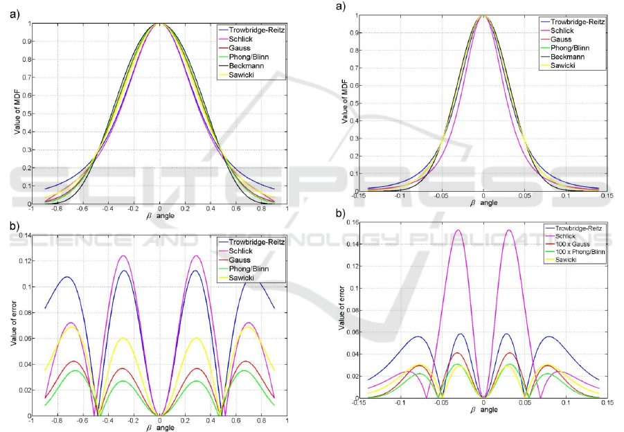
Figs. 1a and 2a show the graphs of the MDFs
discussed for different sets of parameters. Figs. 1b
and 2b show the differences—the relative error
concerned to the maximum value of the function in
relation to Beckmann distribution for the same values
of parameters as in Figs. 1a and 2a.
Figure 1: Graphs of different distribution functions for
parameters calculated based on m
B
=0.4 (N=10, m
G
=0.4364,
C
TR
=0.4456, N
DS
=12.04). a) Values of MDF as a function
of the
β
angle. b) The relative error (as a function of the
β
angle) pertaining to the maximum value of the function in
relation to Beckmann distribution.
Phong’s proposal is a surprisingly good
approximation of the Beckmann distribution. The
max relative error decreases in this case when the N
Phong parameter increases: for N=10, the maximum
relative error is on the level of 3.5%, for N=40 it is
1%, for N=100 is 0.4% and for N=1000 it decreases
to 0.03%. At the same time, it is worth remembering
that MDF is used in modeling of specular reflection
and in practice there are usually values from the range
of N>100.
However, it is noteworthy that a very small
relative error is obtained after replacing the
Beckmann function with the Gauss function (Figs. 1b
and 2b). Many effective approximations of the Gauss
function are well-known, for example, Lee’s
polynomial cubic function (Lee, 2000), the tricube
function (Cleveland and Loader, 1995), and the
Wendland solution (Wendland, 1995). However,
practically, none of these approximations are useful
for the description of the MDF function.
Figure 2: Graphs of different distribution functions for
parameters calculated based on m
B
=0.04464 (N=1000,
m
G
=0.04471, C
TR
=0.05354, N
DS
=1174.3). a) Values of
MDF as a function of the
β
angle. b) The relative error (as
a function of the
β
angle) pertaining to the maximum value
of the function in relation to Beckmann distribution.
In all cases, the functions of Beckmann,
Blinn/Phong, and Gauss are indeed very similar. In
particular, it is noticed for the smooth surface
(N ≥ 1000), when the relative error for Gauss and
Blinn/Phong MDFs are less than 0.05%. Comparing
the graphs (Figs. 1 and 2) and value of RMSE
GRAPP 2021 - 16th International Conference on Computer Graphics Theory and Applications
216

presented in Table 2, it is noteworthy that the
approximation by the Blinn/Phong function is always
better than by the Gauss function. Although both
approximations are very good.
The behavior of the Trowbridge-Reitz distribution
is noteworthy. Its function graph differs considerably
from the Beckmann function. As it shows, the
assumed models of roughness differ from one
another. The unquestionable advantage of the
Trowbridge-Reitz distribution is gentle change in
value for larger angles—“long tail” (Burley, 2012). It
was used in GGX/GTR MDFs. In addition, advantage
is the simplicity of the calculation and the fact that the
integral of the distribution can be analytically
calculated in a simple way, which is sometimes quite
useful in the computational application.
Figure 3: The light reflection from the sphere surface and
graph of luminance on the line of “cross section” through
the spot of light.
In this study, two other MDF representations in a
polynomial/rational form were considered: Schlick
and Sawicki MFD. Both are computationally
attractive. However, both do not give a good
approximation of Beckmann function. The Schlick
function differs significantly from the other MDFs in
all cases. It is the worst solution especially for smooth
surfaces: the maximum relative error of Schlick MDF
is at a level of 13%–15% (in cases presented in Figs.
1b and 2b). A much better result is achieved by
Sawicki MDF, with a relative error of about 3%–7%
(Figs. 1b and 2b).
The evaluation of the implementation of speed of
the MDF functions is worthy of discussion. Blinn
(Blinn, 1977) suggested the Trowbridge-Reitz
polynomial/rational function because of the
improvement in the effectiveness of calculations;
however, in the book (Akenine-Möller et al., 2008),
we can read that such an approximation was
important and relevant while the article was being
written (1977). In my opinion, today this will not be
the main factor determining the choice of MDFs for
the general usage.
4.2 Comparison of Formulas
Graphical Experiments
Experiments with the Ashikhmin-Shirley reflection
model (Ashikhmin and Shirley, 2000) have been
conducted, where different MDFs were used. To
show the differences between the MDFs, the simplest
object has been chosen to make the visual effects and
their interpretation dependent only on the distribution
function used.
A comparison of the visual properties of applying
different MDFs was conducted using an example in
which the light reflection from the sphere surface was
simulated (Fig. 3). To reduce the influence of the
subjective perceptual assessment, the graph of
brightness changes on the line of “cross section”
through the spot of light.
In Fig. 4, the implementation of different MDFs
and graphs of the luminance on the cross section is
shown with the assumption that there was a less
smooth surface (rough), whereas in Fig. 5, different
MDFs are shown with the assumption of very smooth
character. The graph of luminance has been presented
similar to the cross section in Fig. 3, but in order not
to cover stains of light, the line segment is not marked
in Figs. 4 and 5.
As can be seen, according to the expectations,
differences in the appearance of light reflection for
the function of Gauss, Beckmann, and Blinn/Phong
are very small. It is, practically, unnoticeable in the
picture. There are visible changes of colors at
applying the Schlick and Trowbridge-Reitz function:
Schlick because of approximation, Trowbridge-Reitz
because of different model of MDF. The result of the
comparison of the pictures is not surprising if the
differences between shapes of functions are analyzed
(Figs. 1b and 2b). However, these differences do not
change the character of reflection but insert subtle
changes in the reflective properties.
The impact of the Trowbridge-Reitz MDF is
noteworthy, especially for very smooth surface
(Fig. 5). Despite correct conversion of coefficients,
the reflection drawn with the use of the Trowbridge-
Reitz MDF has gentler edges. This fact is used as a
more realistic reflection in the GGX/GTR models.
Microfacet Distribution Function: To Change or Not to Change, That Is the Question
217
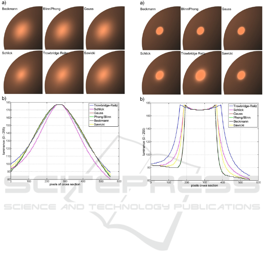
Figure 4: Light reflection from the sphere surface with the
assumption that the surface is rough (less smooth)—
according to Figure 1. a) The view for different microfacet
distribution functions (MDFs). b) The graphs of luminance
on the cross section for used MDFs. Cross section is made
similar to Fig. 3. Graphs for Gauss, Blinn/Phong, and
Beckmann MDFs are so similar that only one line (black) is
visible.
5 CONCLUSIONS
In this article, review of the most important properties
of the MDF that is applied in the BRDF and reflection
models has been presented. Furthermore, the
advantages and disadvantages of those different
MDFs have been considered. The normalized form
for Gauss and Trowbridge-Reitz distribution has been
proposed. Various versions of the rational MDF form
were also analyzed. After RMSE analysis the
mathematical dependencies, that allow for the
exchange of one MDF with the other, have been
proposed.
The answer to the question posed in the title of this
article (to change or not to change) is not so simple.
Figure 5: Light reflection from the sphere surface with the
assumption that the surface is smooth—according to
Figure 1. a) The view for different microfacet distribution
functions (MDFs). b) The graphs of luminance on the cross
section for used MDFs. Cross section is made similar to
Fig. 3. Graphs for Gauss, Blinn/Phong and Beckmann
MDFs are so similar that only one line (black) is visible.
A comparison of different functions shows the
possibility of exchanging one distribution function by
another without the loss of the image quality;
however, it is not always a trivial task. An
examination of Figs. 4 and 5 reveals that reflections
modeling using different MDFs shows very close
effects. Proper conversion of functions parameters is
significant in this case. The introduced and presented
equations and relationship between the parameters of
different MDFs help in this task. However, a deeper
analysis shows a certain small change—subtle
differences. It is particularly visible if the cross
section of the light spot is analyzed (Figs. 4 and 5).
Differences between functions of Beckmann,
Gauss, and Blinn/Phong are unnoticeable, and these
three functions can be used interchangeably in
practically all situations—which is a very important
conclusion from presented here analysis. However,
for these MDFs, it is worth paying attention to the
GRAPP 2021 - 16th International Conference on Computer Graphics Theory and Applications
218

more important problem. Equations (12) – (14)
describe the relationships between the parameters of
these MDFs. For very smooth surfaces,
N
takes
values from a very wide range from about 1000 to
infinity. This corresponds to changes of m
B
(m
G
) in a
very small range. At the same time, for a less smooth
surface (rough surface), we have a relatively larger
range of changes m
B
(m
G
) than
N
. This is due to the
nature of the rational function. This determines a very
practical proposal for its application. For very smooth
surfaces (well reflective), it is worth to use
Blinn/Phong MDF because it is easier to control
reflective properties (subtle changes) with a
parameter in a wider range. In contrast, the Beckmann
(Gauss) MDF is worth using for less smooth surfaces
(poorly reflective).
However, replacing one MDF with another one
can be intentional—to get the proper visual effect.
The application of the Trowbridge-Reitz distributions
causes significant differences in the created
pictures—the visible effect of “long tail” for smooth
surfaces (Fig. 5). This is a significant difference
compared to Beckmann (Gauss, Blinn/Phong) MDF
assuming a similar general nature of changes—
resulting from the conversion of coefficients. This is
a very important advantage of this MDF for modern
applications where GGX/GTR is used. This has also
been confirmed in the publications discussed. A
similar effect to Beckmann, but with subtle “long tail”
for smooth surfaces (Fig. 5) can be obtained with
Sawicki MDF. However, it does not seem that this
MDF can compete with GGX/GTR applications.
Especially if we consider the development of GGX
toward GTR in contemporary studies (Burley, 2012).
Not all MDFs are easy to implement to the same
extent. The Schlick MDF can cause significant
problem because of the range of approximation. The
conversion of Beckmann MDF to Gauss MDF seems
to be justified only in specific situations, if it could
speed up the calculation (which could result from the
use of appropriate similar functions to describe the
material properties). The computational complexity
and the visual properties of both these functions are
practically identical. However, if a function similar to
Beckmann would be needed, but in a
polynomial/rational form, none of the discussed here
two functions make a good approximation.
About MDF, Hall wrote in his book (Hall, 1989)
that “no comparative study has been performed with
these distribution functions.” After approximately 30
years, there is a hope that this article will fill this gap.
REFERENCES
Akenine-Möller, T., Haines, E., Hoffman, N., 2008. Real-
Time Rendering. Third Edition. A K Peters.
Ashikhmin, M., Premože, S., Shirley, P., 2000. A
Microfacet-based BRDF Generator. In: Proc. of
SIGGRAPH’00. 65-74.
Ashikhmin, M., Shirley, P., 2000. An Anisotropic Phong
BRDF Model. Journal of Graphics Tools. 5(2), 25-32.
Bagher, M.M., Soler, C., Holzschuch, N., 2012. Accurate
fitting of measured reflectances using a Shifted Gamma
micro‐facet distribution. Computer Graphics Forum,
31(4). 1509-1518.
Barla, P., Pacanowski R., Vangorp P., 3028. A Composite
BRDF Model for Hazy Gloss. Computer Graphics
Forum. 37(4), 55-56.
Beckmann, P., Spizzichino, A., 1963. The Scattering of
Electromagnetic Waves from Rough Surfaces.
Macmillan, reprint: Artech House (1987).
Bishop, G., Weimer, D., 1986. Fast Phong Shading.
Computer Graphics. 20(4), 103-106.
Blinn, J.F., 1977. Models of Light Reflection for Computer
Synthesized Pictures. In: Proc. of SIGGRAPH’77.
pp.192-198.
Bringier, B., Ribardière, M., Meneveaux, D., Simonot L.,
2020. Design of rough micro-geometries for numerical
simulation of material appearance, Applied Optics
(OSA), 59(16), 4856-4864.
Burley, B., 2012. Physically-Based Shading at Disney. In:
SIGGRAPH 2012 Course: Practical Physically Based
Shading in Film and Game Production.
Chen L., Zheng Y., Shi B., Subpa-Asa A., Sato I., 2017. A
Microfacet-Based Reflectance Model for Photometric
Stereo with Highly Specular Surfaces. In: Proc. of 2017
IEEE International Conference on Computer Vision
(ICCV), 22-29 Oct. 2017. Venice, Italy.
Cleveland, W.S., Loader, C.L., 1995. Smoothing by Local
Regression: Principles and Methods. In: Statistical
Theory and Computational Aspects of Smoothing.
edited by Heardle, W., Schimek, M.G. pp. 10-49.
Springer-Verlag.
Cook, R.L., Torrance, K.E., 1981. Reflectance Model for
Computer Graphics. In: Proc. of SIGGRAPH’81.
pp.307-316.
Dong, Z., Walter, B., Marschner, S., Greenberg, D.P., 2015.
Predicting Appearance from Measured Microgeometry
of Metal Surfaces, ACM Transactions on Graphics
35(1). December 2015.
Dorsey, J., Rushmeier, H.E., Sillion, F.X., 2008. Digital
Modeling of Material Appearance. Morgan Kaufmann.
Embrechts, J.J., 1995. Etude et modélisation de la réflexion
lumineuse dans le cadre de l’éclairage prévisionnel
(English text). PhD thesis. Universite de Liege.
Embrechts, J.J., 1999. Progress in the Modelization of Light
Reflection for Lighting Calculation. In: Proc. of CIE
24th Session – Warsaw’99. pp.194-196.
Hall, R., 1989. Illumination and Color in Computer
Generated Imagery. Springer-Verlag.
He, X.D., 1994. Minor alterations to HTSG model. email
from X.D.He to G.J.Ward, quoted by G.J.Ward in 1994.
Microfacet Distribution Function: To Change or Not to Change, That Is the Question
219

http://groups.google.pl/group/comp.graphics/msg/bc31
74f3df05d9fe?hl=en&. (Accessed 10 January 2020).
He, X.D., Heynen, P.O., Phillips, R.L., Torrance, K.E.,
Salesin, D.H., Greenberg, D.P., 1992. A Fast and
Accurate Light Reflection Model. In: Proc. of
SIGGRAPH’92. pp. 253-254. With related multimedia
paper:
http://www.graphics.cornell.edu/~westin/multimedia-
paper/index.html. (Accessed 10 January 2020).
He, X.D., Torrance, K.E., Sillion, F.X., Greenberg, D.P.,
1991. A Comprehensive Physical Model for Light
Reflection. In: Proc. of SIGGRAPH’91. pp. 175-186.
Heitz, E., 2014. Understanding the Masking-Shadowing
Function in Microfacet-Based BRDFs, Journal of
Computer Graphics Techniques. 3(2). 48-107.
Holzschuch, N., Pacanowski, R,. 2017. A Two-Scale
Microfacet Reflectance Model Combining Reflection
and Diffraction. ACM Transactions on Graphics. 36(4),
Article 66.
Kang, Y.M., Lee, D.H., Cho, H.G., 2015. Multipeak
aniostropic microfacet model for iridescent surfaces.
Multimed Tools Appl. 74(Issue 16), 6229-6242.
Kuijk, A.A., Blake, E.H., 1989. Faster Phong Shading via
Angular Interpolation. Computer Graphics Forum.
8(4), 315-324.
Kurt, M, Edwards, D., 2009. A survey of BRDF models for
computer graphics. ACM SIGGRAPH Computer
Graphics. 43(2), 1-7.
Kurt, M, Szirmay-Kalos, L., Křivánek, J., 2010. An
anisotropic BRDF model for fitting and Monte Carlo
rendering. ACM SIGGRAPH Computer Graphics.
44(1), 1-15.
Lafortune, E.P., Willems, Y.D., 1994. Using the Modified
Phong Reflectance Model for Physicaly Based
Rendering. Tech. Report CW197. Dep. of Computer
Science. Katholieke Universiteit Leuven.
Lee, I.K.,2000. Curve Reconstruction from Unorganized
Points. Computer Aided Design. 17(2), 161-177.
Lengyel, E., 2002. Mathematics for 3D Game
Programming and Computer Graphics. Charles Rover
Media Inc.
Lewis, R.R., 1994. Making Shaders More Physically
Plausible. Computer Graphics Forum. 13(2), 109-120.
Mac Manus, L., Iwasaki, M., Kanamori, K., Sato, S.,
Dodgson, N.A., 2009. Inherent limitations on specular
highlight analysis. The Visual Computer. DOI
10.1007/s00371-009-0331-7
Nicodemus, F.E., 1970. Reflectance Nomenclature and
Directional Reflectance and Emissivity. Applied
Optics. 9(6), 1474-1475.
Nicodemus, F.E., Richmond, J.C., Hsia, J.J., Ginsberg,
I.W., Limperis, T., 1977. Geometrical considerations
and nomenclature for reflectance. NBS Monograph,
NBS (now NIST) October 77.
Neumann, L., Neumann, A., Szirmay-Kalos, L., 1999.
Compact Metallic Reflectance Models. Computer
Graphics Forum. 18(3), 161-172.
Ngan, A., Durand, F., Matusik, W., 2004. Experimental
Validation of Analytical BRDF models, In. Proc. of
SIGGRAPH’04. Technical Sketch.
Ngan, A., Durand, F., Matusik, W., 2005. Experimental
Analysis of BRDF models. In: Eurographics
Symposium on Rendering. pp.117-126. With related
www site:
http://people.csail.mit.edu/addy/research/brdf/index.ht
ml. (Accessed 19 December 2019).
Pharr, M., Jakob, W., Humphreys, G., 2016. Physically
Based Rendering: From Theory to Implementation.
Third Edition. Morgan Kaufmann Publishers Inc.
Phong, B.T., 1975. Illumination for Computer Generated
Pictures. Communications of the ACM. 18(6), 311-317.
Poulin, P., Fournier, A., 1990. A Model for Anisotropic
Reflection. Computer Graphics (SIGGRAPH’90
Proceedings). 24(4), 273-282.
Ribardière, M., Bringier, B., Meneveaux, D., Simonot, L.,
2017. STD: Student's t-Distribution of Slopes for
Microfacet Based BSDFs. Computer Graphics Forum.
36(2), 421-429.
Ribardière, M., Bringier, B., Simonot, L., Meneveaux, D.,
2019. Microfacet BSDFs Generated from NDFs and
Explicit Microgeometry. ACM Transactions on
Graphics, 38(5), Article 143.
Rusinkiewicz, S., 1997. A Survey of BRDF Representation
for Computer Graphics. Report CS348c. Stanford
University.
Sawicki, D., 2006. The New Form of the Microfacet
Distribution Function for the BRDF and Reflection
Models. Przeglad Elektrotechniczny. 82(10), 15-18.
Schlick, Ch., 1994a. A Fast Alternative to Phong's Specular
Model. In: Heckbert P. (ed), Graphics Gems. Vol 4,
pp.363-366. Academic Press.
Schlick, Ch., 1994b. A Survey of Shading and Reflectance
Models. Computer Graphics Forum. 13(2), 121-132.
Schlick, Ch., 1994c. An Inexpensive BRDF Model for
Physically-Based Rendering. Computer Graphics
Forum. 13(3), 233-246.
Strauss, P.S., 1990. A Realistic Lighting Model for
Computer Animators. IEEE Computer Graphics &
Applications. 10(6), 56-64.
Torrance, K.E. Sparrow, E.M., 1967. Theory for Off-
specular Reflection from Roughened Surfaces. Journal
of the Optical Society of America. 57(9), 1105-1114.
Trowbridge, T.S., Reitz, K.P., 1975. Average Irregularity
Representation of a Rough Surface for Ray Reflection.
Journal of the Optical Society of America. 65(5), 531-
536.
Walter, B., Marschner, S.R., Li, H., and Torrance, K.E.,
2007. Microfacet Models for Refraction through Rough
Surfaces. In: Proc. of Eurographics Symposium on
Rendering. pp. 195-206.
Ward, G.J., 1992. Measuring and modeling anisotropic
reflection. ACM SIGGRAPH Computer Graphics
26(2), 265-272.
Ward, G. The Materials and Geometry Format, ver.1.1,
February 1996, http://radsite.lbl.gov/mgf/. (Accessed
15 February 2018)
Wendland, H., 1995. Piecewise polynomial, positive
definite and compactly supported radial functions of
minimal degree. Advances in Comp. Mathematics. 4(1),
389-396.
GRAPP 2021 - 16th International Conference on Computer Graphics Theory and Applications
220
