
A Discrete SIR Model with Spatial Distribution on a Torus for COVID-19
Analysis using Local Neighborhood Properties
Reinhard Schuster
1
, Klaus-Peter Thiele
2
, Thomas Ostermann
3
and Martin Schuster
4
1
Chair of Department of Health Economics, Epidemiology and Medical Informatics, Medical Advisory Board of Statutory
Health Insurance in Northern Germany (MDK Nord), 23554 L
¨
ubeck, Germany
2
Medical Director of the Medical Advisory Service Institution of the Statutory Health Insurance in North Rhine (MDK
Nordrhein), 40212 D
¨
usseldorf, Germany
3
Chair of Research Methodology and Statistics in Psychology, Witten/Herdecke University, Alfred-Herrhausen-Straße 50,
58448 Witten, Germany
4
Faculty of Epidemiology, Christian-Albrechts University Kiel, 24105 Kiel, Germany
martin.schuster@epi.uni-kiel.de
Keywords:
COVID-19, SIR Model, Torus, Differential Equation, Laplace Operator, Mean Value Operator.
Abstract:
The ongoing COVID-19 pandemic threatens the health of humans, causes great economic losses and may
disturb the stability of the societies. Mathematical models can be used to understand aspects of the dynamics of
epidemics and to increase the chances of control strategies. We propose a SIR graph network model, in which
each node represents an individual and the edges represent contacts between individuals. For this purpose, we
use the healthy S (susceptible) population without immune behavior, two I-compartments (infectious) and two
R-compartments (recovered) as a SIR model. The time steps can be interpreted as days and the spatial spread
(limited in distance for a singe step) shell take place on a 200 by 200 torus, which should simulate 40 thousand
individuals. The disease propagation form S to the I-compartment should be possible on a k by k square (k=5
in order to be in small world network) with different time periods and strength of propagation probability in
the two I compartments. After the infection, an immunity of different lengths is to be modeled in the two R
compartments. The incoming constants should be chosen so that realistic scenarios can arise. With a random
distribution and a low case number of diseases at the beginning of the simulation, almost periodic patterns
similar to diffusion processes can arise over the years. Mean value operators and the Laplace operator on the
torus and its eigenfunctions and eigenvalues are relevant reference points. The torus with five compartments is
well suited for visualization. Realistic neighborhood relationships can be viewed with a inhomogeneous graph
theoretic approach, but they are more difficult to visualize. Superspreaders naturally arise in inhomogeneous
graphs: there are different numbers of edges adjacent to the nodes and should therefore be examined in an
inhomogeneous graph theoretical model. The expected effect of corona control strategies can be evaluated by
comparing the results with various constants used in simulations. The decisive benefit of the models results
from the long-term observation of the consequences of the assumptions made, which can differ significantly
from the primarily expected effects, as is already known from classic predator-prey models.
1 INTRODUCTION
The Covid-19 pandemic is a major challenge for phy-
sicians, politicians, scientists and much other groups.
Models are useful to discuss possible scenarios and
implications of interventions to expand background
knowledge and to design policy impact research, cf.
(Chinazzi et al., 2020), (Rosenbaum, 2020), (Pan
et al., 2020), (Behrens et al., 2020), (Tang et al.,
2020).
The contextual selection of adequate models
should be able to generate all known actual and hi-
storic observations by choosing suitable model clas-
ses and parameters, cf. (Bailey, 1975), (Keener and
Sneyd, 1998), (Xue et al., 2020), (Kucharski et al.,
2020). As an intermediate step, the advantages and
disadvantages of known mathematical models in me-
dicine and biology and their implementations in infor-
matics using different classes of parameters should be
analyzed, cf. (Kermack and McKendrick, 1933).
The biomathematical analysis of epidemiological
systems has a long history, cf. (Arnautu et al., 1989),
Schuster, R., Thiele, K., Ostermann, T. and Schuster, M.
A Discrete SIR Model with Spatial Distribution on a Torus for COVID-19 Analysis using Local Neighborhood Properties.
DOI: 10.5220/0010252504750482
In Proceedings of the 14th International Joint Conference on Biomedical Engineering Systems and Technologies (BIOSTEC 2021) - Volume 5: HEALTHINF, pages 475-482
ISBN: 978-989-758-490-9
Copyright
c
2021 by SCITEPRESS – Science and Technology Publications, Lda. All rights reserved
475

(Aronson, 1985), (Beretta and Capasso, 1986). The
family of SIR models with various generalizations of
the status elements S (susceptible), I (infected or in-
fectious) and R (removed or recovered) with respect
to other status elements as E (exposed) and subpopu-
lations use ordinary differential equations, cf. (Ahmed
and Agiza, 1998), (Andersen and May, 1979), (Capas-
so, 1993), (Redheffer and Walter, 1984).
The variables are fractions of the population mo-
delled as positive real numbers as in the mass acti-
on law supposing homogeneous distributions. Peri-
odic solutions of first order ordinary differential equa-
tions are unstable with respect to system parameters.
A large number of SIR models use bilinear differenti-
al equations, cf.(R
¨
udiger et al., 2020).
We propose a model which could be presented as
a cellular automata. In order to use methods of par-
tial differential equations and mean value operators
in differential geometry we use differential manifolds
as a general modelling background and its discreti-
zation which generalizes the Euclidean structure of
cellular automata, cf. (Mikeler et al., 2005), (G
¨
unther
and Pr
¨
ufer, 1999), (Schuster, 1988), (Schuster, 1997),
(Wang et al., 2015), (Welch et al., 2011).
An essential feature will be the visualization of de-
velopment of the pandemic with special structures, cf.
(Murray, 2002), (Murray, 2003), (Barrat and Vespig-
nani, 2008), (Andersen and May, 1979). This will be
realized with Mathematica from Wolfram Research
which also allows to use a syntax without coordinates.
A visualization of the pandemic status of 40 thousand
individual can be reached with some hours of calcula-
tion time. The results to be considered in the followi-
ng have proven to be the optimal solution within the
used simulations with regard to the target variable that
is still to be discussed.
If one would change the discretization of the torus
structure of the used differential manifold by a graph
structure (cf. (Solimano and Bretta, 1982), (R
¨
udiger
et al., 2020), (Welch et al., 2011), (Boguna et al.,
2003)) much less individuals could be visualized.
Cyclical structures in the sense of a boundary cy-
cle or a cyclical band were discussed in chemical
and biological examples, where there are fundamen-
tal theoretical differences, but also commonalities bet-
ween discrete and continuous systems, cf. (Capas-
so and Maddalena, 1983), (Field and Burger, 1985).
When modeling exponential growth, there are not on-
ly differences between continuous and discrete sy-
stems, but also between spatially bounded and un-
bounded systems (compact and non-compact mani-
folds in differential geometry), cf. (Murray, 2002),
(Murray, 2003), (Barrat and Vespignani, 2008), (Be-
retta and Capasso, 1986), (Boguna et al., 2003), (So-
limano and Bretta, 1982). In this context, the r-value
plays a role in the current Covid-19 discussion that
has already been analyzed earlier in various contexts,
cf. (Dieckman et al., 1990). The r-value should de-
scribe the prevailing value of an exponential spread.
The exponential mapping provides the crucial relati-
onship between Lie algebras and Lie groups in diffe-
rential geometry. This goes far beyond the exponen-
tial function on real numbers, which already shows a
completely different qualitative behavior on complex
numbers. Using the exponential function to describe
the spread of Covid-19, which could practically ne-
ver be sensibly modeled with an exponential spread,
leads to theoretical and practical problems. The expo-
nential map on a discretized torus leads to a growth in
which the saturation value has to be estimated, which
is in principle impossible from short initial data. The
actual paper is a first step in the stated context.
2 MATERIAL AND METHODS
Individuals are the elements of an n by m array (in the
examples we use the special values n = m = 200). In-
dividuals can be in the status S (susceptible: healthy
without immune behavior), I
1
or I
2
(infected or infec-
tious after incubation period) and R
1
or R
2
(recovered
with immune behavior) for each day after initializa-
tion. Further on for every individual in the I
1
, I
2
, R
1
or R
2
status the number of days being in that status is
considered, cf. Figure 1. It is also possible to model
different immune behavior specifically related to the
infectious disease in different S compartments, here
this is be done in the R compartments.
The right and left hand as well as the upper and
lower elements of the array resulting from the dis-
cretization of the torus are connected. If one would
change the upper and lower side of the right and left
sides of the array and respectively for the upper and
lower side we would get the discretization of double
M
¨
obius strip which can’t be realized in three dimen-
sional geometry. With an other boundary identificati-
on one also could reach the topology of a sphere.
As a local neighborhood of the array element (i, j)
we consider all elements (i + k, j + k) mod n with
−m ≤ k ≤ m (m = 5 in the examples). An S indivi-
dul in the local neighborhood of a I individual is in-
fected randomly with equal probability with the pro-
perty that during the infectious period r individuals (r
as the theoretical reproduction number) are infected.
This theoretical reproduction number supposes that
all other individuals in the local neighborhood are in
the S status.
The individuals of the I
2
compartment are less in-
HEALTHINF 2021 - 14th International Conference on Health Informatics
476

S
I
2
I
1
R
1
R
2
p
1
p
2
p
5
p
6
p
7
p
8
p
3
p
4
p
9
p
10
2
Figure 1: SIR compartments and transitions p.
fectious than those of the I
1
compartment but over a
longer period of time, both lead to the same resulting
reproduction number in the used simulation. This as-
sumption can be modified.
The individuals of the R
2
compartment should be
immune longer than those individual of the R
1
com-
partment. At the beginning of the simulation, all indi-
viduals should belong to the S compartment with the
exception of i
1
and i
2
individuals, respectively, ran-
domly determined individuals of the I
1
and I
2
com-
partments. The previous time in the I
1
or I
2
compart-
ment should also be chosen randomly. This means
that at the beginning of the observation of the spread
there is no immune behavior. With regard to measures
to be taken to limit the spread of the infection, this is
the most unfavorable option. Alternatively, one could
start with an initial distribution of individuals in R
1
and R
2
compartments. Since simulations have shown
that the same dynamic behavior will occur in the me-
dium term, it was easier to choose comparable initial
conditions.
After the infectious period of individuals of I
1
or
I
2
they change to R
1
or R
2
individuals by transiti-
on parameters. After immunity, the individuals switch
back to the S compartment. There also may be a
switch between I
1
and I
2
individuals. The transitions
p
i
(i=1,...10) between the compartments are shown
in Figure 1. In the considered context the p
i
are sto-
chastic processes depending on the previous length of
stay of the individuals of the compartments. In an ana-
log Markov model, these are only transition probabi-
lities.
The daily steps are simultaneously using the pre-
vious day’s conditions for all transitions. This inclu-
des that an individual in an R-compartment which
changes to the S-compartment can not change from
another individual to an S-compartment through in-
fection during this step. In this way, an overall effect
of all other individuals in the local contagious neigh-
borhood is achieved.
S individuals may be infected by all I
1
or I
2
indi-
viduals in the related local neighborhood with resul-
ting increasing probability with the number of these
individuals, similar to a bilinear infection in SIR mo-
dels without spacial structure. Thereby the new I
1
or
I
2
individuals are determined. After that step R
1
or R
2
individuals may switch to S individuals and I
1
or I
2
individuals may switch to R
1
or R
2
individuals. The
parameters of the simulation should be determined in
such a way that
1. the I
1
compartment is as small as possible
2. the transition probability from the S compartment
to the I
2
compartment (long infectious) is smal-
ler than that into the I
1
compartment (short infec-
tious) and
3. a large proportion of the population reaches the R
1
or R
2
compartment.
Small I compartments and large R compartments are
opposing objectives, since only I individuals can be-
come R individuals. I
1
individuals can be interpreted
as symptomatic cases or as individuals with stronger
disease symptoms and I
2
individuals as asymptoma-
tic cases or with lower disease symptoms. We want
to reach large immunity with low treatment cases as a
target. The system should be able to generate appro-
ximately stable cyclical behavior (including a cyclic
band with chaotic behavior in the inner band part),
because states of equilibrium can be unstable possib-
ly solely through external influences.
Of central interest is how the system settles. If the
first or second oscillation (first or second wave) is si-
gnificantly higher than later oscillations of small am-
plitude for the diseases, a new infection from outside
is a high risk as immunity declines. A small regular
rate of contamination from outside should realistical-
ly be included in the model.
The approach considered is a discretization of a
partial integro-differential equation with an additional
time delay. The effect of the local environment can be
viewed as a mean value operator. It is known from
differential geometry that the eigenvalues of the La-
place operator are also eigenvalues of the mean value
operators and that eigenfunctions of the mean value
operators and can be calculated from those of the La-
place operator, with no time delays being included in
the considerations of differential geometry. Instead of
the time delays, as is usual in SIR models, transition
probabilities can be replaced, which can be modeled
as reciprocal values of the expected value of remai-
ning time in the compartment.
A Discrete SIR Model with Spatial Distribution on a Torus for COVID-19 Analysis using Local Neighborhood Properties
477

3 RESULTS
We start with 10 randomly infected individuals of the
I population, all other individuals should initially be
in the S compartment. This number is important with
regard to the number of initial clusters of the infection
and should initially model a low external influence. A
small number extends the initial phase, a high number
induces a dynamic that has to be synchronized with an
approximately periodically stable internal system dy-
namic. Half of the individuals in the I compartment
should initially be in the I
1
compartment, the other in
the I
2
compartment. An incubation period is not inclu-
ded in the results considered here, but in the previous
simulations they have not led to any other qualitative
results. These only show changes in the initial phase
of the development of the infection.
The results of this section are calculated with the
optimal parameters with respect to the mentioned goal
to reach low infections over the time including the in-
itial phase and a large number of immune individuals
over the time out of over 100 long time simulations.
In addition to the spatial distributions and progress fi-
gures in the individual compartments, we will provi-
de qualitative comparisons with the other simulations
carried out.
Individuals in the I
1
compartment should be con-
tagious for two weeks, and individuals in the I
2
com-
partment for 10 weeks, this is a ratio of 5. Other ratios
have shown less stable results or worse results in re-
lation to the main target.
Due to the large number of incoming parameters,
the search for an optimum was only able to find a lo-
cally optimal version. Further theoretical analyzes are
necessary at this point.
The time unit primarily used is also to be regarded
as provisional. The need for an adjustment may arise
from the cycle durations resulting from the long-term
behavior.
The r-value of the RKI (Robert Koch institute) of-
ten used in Germany results from ratios of two latest
available consecutive three day incidence numbers. If
the used time step is shorter than a day the r-value
becomes more stable.
Every individual of the I
1
population shall have
a theoretical (initial) r-value of 3. This shall men,
that this individual would infect 3 other individuals
throughout his infection period, if all individuals in
the considered local neighborhood under considerati-
on belonged to the S compartment. Half of the newly
infected individuals should get into the I
1
and I
2
com-
partments.
One could assume that smaller theoretical initial
r-values would be desirable. As a result of the mo-
re slowly developing immunity, however, they lead to
more diseases in the initial phase and to higher long-
term stability with repeated high numbers of diseases.
High initial r-values lead to high values in the I
1
com-
partment, with an interpretation that leads to high ca-
se numbers in hospital care and should therefore be
avoided as a priority. The proportion of hospital cases
within the I
1
compartment is not considered here, as it
has at most a marginal effect on the spread dynamics.
Individuals in the I
2
compartment should only be
5% as contagious as individuals in the I
1
compart-
ment, with half of the new infections reaching the I
1
and I
2
compartments. But this I
2
compartment has a
major influence on the dynamics of the spread, as the
longer residence time in this compartment has a sta-
bilizing effect on the spatial distribution of the com-
partments. If dynamic differences between the I
1
and
I
2
compartments are too small, there is no spatial sta-
bilization effect. If the differences are too large, the
overall effect of the I
2
compartment is too small. In
between there is at least a local optimum with regard
to the central target variable with regard to the ratio
considered here.
In addition, there should be an external possibili-
ty of infection. Complete isolation of a region is an
illusion, especially with regard to asymptotic cases,
and would only lead back to the unfavorable settling
phase.
Every fifth day a randomly selected individual is
infected if this is in the S compartment. This results
in a slight acceleration in the initial phase of the dy-
namics of the epidemic and has almost no effect if the
immune behavior is widespread. This approach pre-
vents the infection from escalating under the illusion
that a region can be completely isolated from the out-
side world.
R-value = 1.10, day = 91
0 → 38 899
1 → 204
2 → 808
3 → 613
4 → 78
R-value = 0.99, day = 182
0 → 32 755
1 → 580
2 → 2545
3 → 4347
4 → 375
R-value = 0.97, day = 273
0 → 25 510
1 → 349
2 → 2497
3 → 11 392
4 → 854
R-value = 0.98, day = 365
0 → 22 634
1 → 119
2 → 918
3 → 15 851
4 → 1080
Figure 2: S-I-R compartments at day 91, 182, 273 and 365
(from top left to bottom right).
HEALTHINF 2021 - 14th International Conference on Health Informatics
478
After the contagion phase, 90% of the individuals
in the I
1
compartment should be randomly selected to
move to the R
1
compartment, the rest to the R
2
com-
partment. Based on the I
2
compartment, it should be
80% respectively. A thoroughly interesting interacti-
on between the I
1
and I
2
compartments is initially not
considered here, since this results in a strong interac-
tion with regard to a meaningful determination of the
parameters to be used and significantly extends the
search process for meaningful combinations. The in-
dividuals in the R
1
compartment should remain there
for 180 days (about half a year), those in the R
2
com-
partment for three times that time. With these parame-
ters, after one quarter (91 days), the division into the
S-I-R compartments is shown in Figure 2 top left. The
colors are those used in Figure 1. The S compartment
with value 1 is shown in yellow. The I
1
compartment
is shown in lighter red (value 2) and I
2
in darker red
(value 3). Intuitively, red should act as a warning color
according to the traffic light symbols. The temporari-
ly immune compartment is shown in green, the lighter
green (value 4) with shorter immunity than the darker
green (value 5).
The specified r-value in the figure is the value
used by the RKI (Robert-Koch Institute in Germany),
which describes the ratio of new infections from two
consecutive 3-day periods. If you follow the results
in detail, you can quickly see that this value descri-
bes the development of the infection very poorly and
misleadingly in the used simulation.
The epidemiological situation of the next quarter
(day 182) is described in Figure 2 top right.
In this simulation, over 75% of the population is
not yet affected by the epidemic. It can be seen to
a large extent through the strong creative power of
random processes caused the emergence of distribu-
tion patterns. Pattern creation has been discussed in
mathematical modeling in chemical, biological and
medical applications for many decades, especially in
the case of diffusion effects, and is relevant to the
approach considered here, cf. (Murray, 2002), (Mur-
ray, 2003), (Aronson, 1985), (Capasso and Madda-
lena, 1983). The Laplace operator already discussed
plays a decisive role in diffusion processes. Spectral
results (eigenvalues and eigenvectors) of the Laplace
operator are relevant for pattern formation.
Regarding the strong design ability of random
processes, it should be noted that with random primes
it was possible to depict properties of prime numbers
as motivated, the proof of which has not been suc-
cessful for hundreds of years. Why this is so is largely
unclear and is a challenge for future research. These
considerations are not based on simulations, but on
calculations using the stochastic approach. Such an
approach is also useful for the present topic.
The epidemiological situation of the next quarter
(day 273) is described in Figure 2 bottom left.
About half of the population is affected by the epi-
demic. The pattern emergence is largely shaped by the
previous quarter. One year after the start of the simu-
lation, a high level of immunity is achieved, although
this is associated with few new infections.
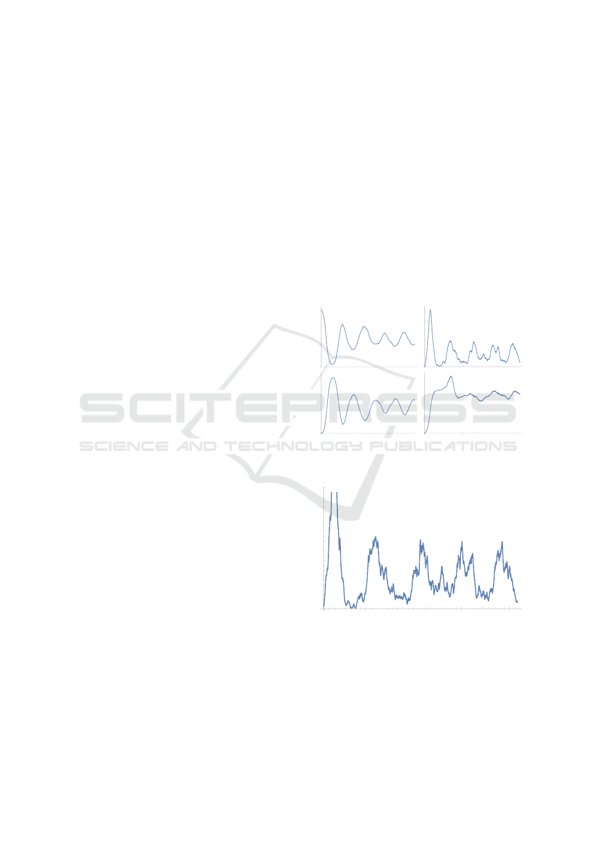
Before details of the next few years are presented,
the time series in the compartments should be consi-
dered in Figure 3. After a large initial swing, the S-
compartment stabilizes at approx. 75% of the popula-
tion with a variation of approx. 25% of the population
in the considered simulation.
As shown in Figure 3 the I
2
compartment shows
significantly lower amplitudes than the I
1
compart-
ment.
500 1000 1500 2000 2500 3000 3500
25 000
30 000
35 000
40 000
S compartment
500 1000 1500 2000 2500 3000 3500
500
1000
1500
2000
2500
3000
I2 compartment
500 1000 1500 2000 2500 3000 3500
5000
10 000
15 000
R1 compartment
500 1000 1500 2000 2500 3000 3500
500
1000
1500
R2 compartment
Figure 3: Time series of the S compartment (top left), I
2
compartment (top right), R
1
compartment (bottom left) and
R
2
compartment (bottom right).
500 1000 1500 2000 2500 3000 3500
100
200
300
400
500
I1 compartment
Figure 4: Time series of the I
1
compartment.
While the I
1
and I
2
compartments show a high de-
gree of correspondence over time, there are signifi-
cant qualitative differences for the R
1
and R
2
com-
partments.
After some years, the epidemic system is still in
the settling phase.
In the years nine and ten after the start of the simu-
A Discrete SIR Model with Spatial Distribution on a Torus for COVID-19 Analysis using Local Neighborhood Properties
479

R-value = 0.80, day = 730
0 → 32 374
1 → 47
2 → 266
3 → 6713
4 → 1202
R-value = 1.03, day = 1095
0 → 28 773
1 → 171
2 → 919
3 → 9379
4 → 1360
R-value = 1.01, day = 3285
0 → 32 635
1 → 233
2 → 1001
3 → 5762
4 → 971
R-value = 1.04, day = 3650
0 → 29 073
1 → 32
2 → 231
3 → 10 233
4 → 1033
Figure 5: S-I-R compartments after 2, 3 9 and 10 years
(from top left to bottom right).
lation, the epidemic essentially shows the long-term
dynamics.
If the time step is really shorter than one day, then
the number of years for the settling process is corre-
spondingly shorter. For long-term observations, annu-
al influences on the assumed constants of infection are
relevant. This process of synchronization between the
internal clock and the external clock has long been
discussed in the biomathematical literature and will
be taken up in a later paper.
4 DISCUSSION AND
CONCLUSIONS
The dynamics of the development of the epidemic is
influenced by the interaction of all parameters used.
Only then does it become apparent whether the time
unit used is compatible with the observation. The re-
sults suggest that the time unit used is significantly
shorter than a day and thus the observation period is
shorter than ten years. This implies that the given RKI
r-value becomes more stable without its fundamen-
tal problem changing. The r-value varies at relative-
ly short intervals between values below and above 1.
The simulations show that it has no significance for
the formation of new regional clusters. Regional clu-
sters can trigger regional interventions with a suitable
scaling, which, however, as already mentioned, can
be counterproductive to the development of immune
behavior. To make matters worse, only the I
1
com-
partment is visible, but the dynamics are essentially
determined by the entire I compartment. This natu-
rally also raises the question of whether the r-value
(real and in the simulation) should be calculated with
the entire I compartment or only with the I
1
compart-
ment. The entire I compartment is useful for the si-
mulation, but only the I
1
compartment is practical-
ly measurable. A further complication arises becau-
se there are no representative estimated values for the
population, but Covid-19 test results are only availa-
ble through measures that are essentially politically
selective. Tracking Covid-19 contact chains with ex-
tensive quarantine can limit the positive development
of immunity by the I
2
population. Since this happens
predominantly, only selectively, it will only lead to a
few spatial disparities that are already present through
pattern creation processes.
Infectious diseases often vary from season to sea-
son. This can be implemented in the model in that the
transition probability used are subject to a seasonal
course. However, this only makes sense if the time
unit resulting from the combination of the parameters
used has been adapted sufficiently reliably to real ti-
me units. The synchronization of different time sca-
les poses is a challenge for future research. The mo-
deling on the torus could be extended by bifurcation
at certain points or intervals, which leads to a direc-
ted graph in the graph-theoretical interpretation. This
could be used to model the interaction of distant con-
tinents.
We considered a delay model in the simulation un-
der consideration. In a subsequent analysis it is ex-
amined whether the qualitative behavior of the simu-
lation is retained if the length of stay in the compart-
ments is replaced by transition probabilities. In mo-
dels of ordinary and partial differential equations, de-
lays generally lead to qualitatively significantly diffe-
rent results.
If Markov models lead to qualitatively similar re-
sults in the context used for the epidemiological situa-
tion under consideration, eigenvalues and eigenfunc-
tions of the corresponding analytical manifolds could
be helpful for analyzing the stability of the parameters
used.
With suitable boundary conditions, eigenvalues
and eigenfunctions of the Laplace operator are well
known for the torus under consideration. The Laplace
operator is decisive for diffusion processes that play
a decisive role and leads to morphological develop-
ments in pattern formation, cf. (Murray, 2002), (Mur-
ray, 2003). Mean value operators in the sense of diffe-
rential geometry have not yet been used in mathemati-
cal biology. In differential geometry and the theory of
relativity, they are used to characterize spatial structu-
res, cf. (G
¨
unther and Pr
¨
ufer, 1999), (Schuster, 1988),
(Schuster, 1997). In the simulation under considerati-
on, we used mean value operators with a uniform dis-
tribution in the maximum metric used. The equal dis-
HEALTHINF 2021 - 14th International Conference on Health Informatics
480

tribution can be replaced by other distributions which,
in a possibly more realistic way, reduce the risk of in-
fection with increasing distance. Again, this is only
partially realistic because life does not take place on
a torus and there are different near-far relationships
that can be analyzed with graph-theoretic methods, cf.
(Solimano and Bretta, 1982), (R
¨
udiger et al., 2020),
(Welch et al., 2011), (Boguna et al., 2003), (Barrat
and Vespignani, 2008).
It is also of essential importance in which way the
”
small world model“ is used, in which it is described
in which
”
small“ number of steps each individual can
be reached by any other individual, here relevant for
chains of infection. In the present context, however,
a theoretically possible path must be supplemented
with a probability with which this path will be im-
plemented in practice.
In a subsequent paper we will analyze the consi-
dered epidemiological development on real life graph
networks. As a small network we will use anonymi-
zed physicians as nodes of the graph, the edges are gi-
ven by a through a neighborhood relationship in terms
of the number of common patients. As a large network
we will use anonymized patients related by physicians
visited by both patients using a random selection. In
graph theory one also can use the Laplace operator
and mean value operators.
Current virological results on Covid-19, as stated
in (Chinazzi et al., 2020), (Rosenbaum, 2020), (Pan
et al., 2020), (Behrens et al., 2020), (Tang et al.,
2020), (Xue et al., 2020), (Kucharski et al., 2020) may
influence the spatial-temporal modeling on the level
of individuals in future and will give new insights in
the dynamics of propagation. But the dynamic of the
contagion occurs to a certain extent independently of
the knowledge of the known details on an individual
level. The influence of measurable variables in indivi-
dual contacts on global expansion and their validation
is a challenge for future research.
It could be that the currently predominantly used
PCR tests identify the individuals in the I
1
compart-
ment in our interpretation or the individuals that have
already passed into the R compartment. The dynamics
observed could indicate that, due to cross immunity
or other immunological mechanisms, that the I
2
com-
partment, which could be very important for the dy-
namics of spread, has so far been little identified in
practice.
In different countries there were different drama-
tic initial situations in the early phase of Covid-19.
So far, this has been largely discussed as the result of
various politically decided preventive measures. But
it could also be that different initial conditions exi-
sted with regard to the R-compartment as a result of
pre-existing immunity. As already stated, an overar-
ching cross-immunity with regard to Covid-19 could
also be modeled in the S compartment. This would ha-
ve theoretical advantages, but would make the search
for meaningful parameters for modeling based on the
current state of knowledge more difficult.
Differing spreading dynamics, regardless of the
measures taken, may also have played a role.
If measures are aimed at greatly reducing the con-
tagion, this subsequently leads to poor immunity at
least without effective vaccinations. Since the contact
restriction was practically inconsistent, sufficient im-
munity was nevertheless not prevented with the ex-
ception of very restrictive measures in some coun-
tries, which may have since led to a high second wave.
The amount of people in overcrowded local transport
means may be seen in different interpretations. Cur-
rent observations can be interpreted to the effect that
particularly drastic contact restrictions due to immu-
nity not being achieved could lead to a second wave.
The compartment status has a discrete value (S, I
1
,
I
2
, R
1
, R
2
), while eigenfunctions and their discretiza-
tions have a real values. If one intends to use the me-
thod of separating the variables to carry out a series
expansion using the eigenvalues of the Laplace opera-
tor, additional considerations are necessary. A similar
problem arises in the bisection problem of graphs. A
good starting solution is to separate the eigenfunction
for the largest non-trivial eigenvalues into points with
positive and negative values. In this respect, it could
be a sensible approach to use the eigenfunctions for
suitable eigenvalues in a hierarchical procedure (since
there are more than two discrete states) for the identi-
fication of inherently periodic solutions.
REFERENCES
Ahmed, E. and Agiza, H. (1998). On modeling epidemics,
including latency, incubation and variable susceptibi-
lity. Physica A, 253:347–352.
Andersen, R. and May, R. (1979). Population biology of
infectious diseases. Part I. Nature, 280:361–367.
Arnautu, V., Barbu, V., and Capasso, V. (1989). Controlling
the spread of epidemics. Appl.Math.Optimiz., 20:297–
317.
Aronson, D. (1985). The role of diffusion in mathematical
population biology: Skellam revisited. Lecture Notes
in Mathematics 57 (eds. Capasso, V., Grosso, E. and
Paveri-Fontana, S.L.).
Bailey, N. (1975). The Mathematical Theory of Infectious
Diseases. Griffin, London.
Barrat, R. and Vespignani, M. (2008). Dynamical Processes
on Complex Networks. Cambridge University Press.
Behrens, G., Cossmann, and A. Stankov, M. V. e. (2020).
A Discrete SIR Model with Spatial Distribution on a Torus for COVID-19 Analysis using Local Neighborhood Properties
481

Perceived versus proven SARS-CoV-2-specific im-
mune responses in health-care professionals. Infec-
tion, pages 631–634.
Beretta, E. and Capasso, V. (1986). On the general struc-
ture of epidemic systems. global asymptotic stability.
Comp. and Maths. with Apps., 12A:677–694.
Boguna, M., Pastor-Satorras, A., and Vespignani, A. (2003).
Epidemic spreading in complex networks with de-
gree correlations, in: Statistical Mechanics of Com-
plex Networks. Lecture Notes in Physics, vol. 625.
Capasso, V. (1993). Mathematical Structures of Epidemic
Systems. Lecture Notes in Biomathematics 97.
Capasso, V. and Maddalena, L. (1983). Periodic solutions
for reaction-fiffusion system modelling the spread of a
class of endemics. SIAM J. Appl. Math., 43:417–427.
Chinazzi, M., Davis, J., and Ajelli, M. e. a. (2020). The ef-
fect of travel restrictions on the spread of the 2019 no-
vel coronavirus (COVID-19) outbreak. Science, 368
(6489):395–400.
Dieckman, O., Heesterbeek, J., and Metz, J. (1990). On the
definition and the computation of the basic reproduc-
tion ratio R0 in models for indectious diseases in he-
terogeneous populations. J.Math.Biol., 28:365–382.
Field, R. and Burger, M. E. (1985). Oscillations and Tra-
veling Waves in Chemical Systems. John Wiley, New
York.
G
¨
unther, P. and Pr
¨
ufer, F. (1999). Mean Value Operators,
Differential Operators and D’Atri Spaces. Annals of
Global Analysis and Geometry, 17:113–127.
Keener, J. and Sneyd, J. (1998). Mathematica Physiology.
Springer, New York.
Kermack, W. and McKendrick, A. (1933). Contri-
butions to the mathematical theory of epidemics.
Proc.R.Soc.Lond.A, pages 94–122.
Kucharski, A., Russell, T., and Diamond, C. e. (2020). Early
dynamics of transmission and control of COVID-19: a
mathematical modelling study. The Lancet infectious
diseases.
Mikeler, A., Venkatachalam, S., and Abbas, K. (2005). Mo-
delling Infectious Diseases Using Global Staochastic
Cellular Automata. Journal of Biological Systems,
13:421–439.
Murray, J. (2002). Mathematical Biology, I: An Introducti-
on. Springer New York Berlin Heidelberg.
Murray, J. (2003). Mathematical Biology, II:Spacial Mo-
dels and Biomedical Applications. Springer New York
Berlin Heidelberg.
Pan, A., Liu, L., and Wang, C. e. a. (2020). Association
of publichealth interventions with the epidemiology
of the COVID-19 outbreak in Wuhan, China. JAMA,
323:1–9.
Redheffer, R. and Walter, W. (1984). Solution of the stabi-
lity problem for a class of generalized volterra prey-
predator systems. J.Diff.Equations, 52:245–263.
Rosenbaum, L. (2020). Facing Covid-19 in Italy - ethics,
logistics, and therapeutics on the epidemic’s frontline.
N Engl J Med., 382:1873–1875.
R
¨
udiger, S., Plietzsch, F., Sokolov, I., and Kurths, J. (2020).
Epidemics with mutating infectivity on small-world
networks. Scientific Reports, 10 (1):1–11.
Schuster, R. (1988). On differential equations related to
mean value operators for differential forms in hyper-
bolic spaces and applications to problems in spectral
geometry. Prace Naukowe Politechniki Szczecinskiej,
380:225–251.
Schuster, R. (1997). About Systems of Differential Equa-
tions related to geodesic differential forms. Mean va-
lues and harmonic spaces. Part I. Journal for Analysis
and its Applications, pages 83–106.
Solimano, F. and Bretta, E. (1982). Graph theoretical crite-
ria for stability and boundedness of predator-prey sy-
stems. Bull Math. Biol., 44:579–585.
Tang, B., Wang, X., and Li, Q. e. a. (2020). Estimation of
the transmission risk of the 2019-ncov and its implica-
tion for public health interventions. Journal of clinical
medicine, 9 (2):462.
Wang, Y., Cao, J., and Alofi, A. e. (2015). Revisiting node-
based sir models in complex networks with degree
correlations. Physica A, 437:75–88.
Welch, D., Bansal, S., and Hunter, D. (2011). Statistical
inference to advance network models. Epidemics, 3
(1):38–45.
Xue, F., Jing, S., and et.al., M. J. (2020). A data-driven net-
work model for the emerging COVID-19 epidemics in
wuhan, toronto and italy. Mathematical Biosciences,
326:108391.
HEALTHINF 2021 - 14th International Conference on Health Informatics
482
