
Beneficial Effect of Combined Replay for Continual Learning
M. Solinas
1
, S. Rousset
2
, R. Cohendet
1
, Y. Bourrier
2
, M. Mainsant
1
, A. Molnos
1
, M. Reyboz
1
and M. Mermillod
2
1
Univ. Grenoble Alpes, CEA, LIST, F-38000 Grenoble, France
2
Univ. Grenoble Alpes, Univ. Savoie Mont Blanc, CNRS, LPNC, Grenoble, France
{yannick.bourrier, stephane.rousset, martial.mermillod}@univ-grenoble-alpes.fr
Keywords:
Incremental Learning, Lifelong Learning, Continual Learning, Sequential Learning, Pseudo-rehearsal,
Rehearsal.
Abstract:
While deep learning has yielded remarkable results in a wide range of applications, artificial neural networks
suffer from catastrophic forgetting of old knowledge as new knowledge is learned. Rehearsal methods over-
come catastrophic forgetting by replaying an amount of previously learned data stored in dedicated memory
buffers. Alternatively, pseudo-rehearsal methods generate pseudo-samples to emulate the previously learned
data, thus alleviating the need for dedicated buffers. Unfortunately, up to now, these methods have shown
limited accuracy. In this work, we combine these two approaches and employ the data stored in tiny mem-
ory buffers as seeds to enhance the pseudo-sample generation process. We then show that pseudo-rehearsal
can improve performance versus rehearsal methods for small buffer sizes. This is due to an improvement in
the retrieval process of previously learned information. Our combined replay approach consists of a hybrid
architecture that generates pseudo-samples through a reinjection sampling procedure (i.e. iterative sampling).
The generated pseudo-samples are then interlaced with the new data to acquire new knowledge without forget-
ting the previous one. We evaluate our method extensively on the MNIST, CIFAR-10 and CIFAR-100 image
classification datasets, and present state-of-the-art performance using tiny memory buffers.
1 INTRODUCTION
Machine learning is being increasingly used to pro-
cess information generated by standalone devices
which operate at the edge of operators’ networks
and have limited or no access to centralized services.
Thanks to edge computing, which brings computation
and data storage closer to where data is generated,
data can be processed faster thus reducing costs and
enabling smarter local decision-making. In this con-
text, edge computing performs continuous operations
and requires continual learning (CL) machine learn-
ing models that gradually extend acquired knowledge
for future decision-making.
While the human brain exemplifies such dynamic
behavior by continuously learning new concepts,
this major feature becomes impracticable for clas-
sic learning models based on neural networks. In-
deed, artificial neural networks (ANNs) are not able
to learn incrementally because they suffer from catas-
∗
This work has been partially supported by
MIAI@Grenoble Alpes, (ANR-19-P3IA-0003).
trophic forgetting of old knowledge as new knowl-
edge is learned (McCloskey and Cohen, 1989). Thus,
ANNs are incapable of updating their knowledge over
time without forgetting previously learned informa-
tion.
In continual learning, the easiest way to overcome
catastrophic forgetting is to learn new training sam-
ples jointly with old ones. The best and simplest solu-
tion is to store all the previously seen samples; how-
ever, this solution is unrealistic and requires a large
memory footprint often impracticable for edge or em-
bedded devices. Replay methods, which consist in
replaying old samples while learning new ones, were
proposed several years ago to solve the catastrophic
forgetting problem in sequential learning scenarios
(Robins, 1995). They were originally divided into re-
hearsal and pseudo-rehearsal methods depending on
the way the old samples were acquired.
Rehearsal methods using only a fraction of old
samples have recently been found to be one of the best
solutions to alleviate the catastrophic forgetting prob-
lem (De Lange et al., 2019; Chaudhry et al., 2019;
Prabhu et al., 2020) due to their ability to succes-
Solinas, M., Rousset, S., Cohendet, R., Bourrier, Y., Mainsant, M., Molnos, A., Reyboz, M. and Mermillod, M.
Beneficial Effect of Combined Replay for Continual Learning.
DOI: 10.5220/0010251202050217
In Proceedings of the 13th International Conference on Agents and Artificial Intelligence (ICAART 2021) - Volume 2, pages 205-217
ISBN: 978-989-758-484-8
Copyright
c
2021 by SCITEPRESS – Science and Technology Publications, Lda. All rights reserved
205

sively integrate new knowledge (i.e. limitless plas-
ticity) (De Lange et al., 2019) and to their superior
performance compared to other CL methods given a
similar amount of computational resources. To main-
tain previous information, rehearsal methods require
a buffer to store previously seen samples and, surpris-
ingly, they still work well when using only a tiny frac-
tion of the previous samples (Chaudhry et al., 2019),
which we denote as tiny memory buffers. The small
memory footprint of theses solutions justifies their el-
igibility for embedded applications.
Alternatively, pseudo-rehearsal methods (Robins,
1995; Ans and Rousset, 1997; Lavda et al., 2018;
Lesort et al., 2019) were conceived to avoid the uti-
lization and storage of previously learned samples.
Instead of replaying past training data from buffers,
a complementary learning system approximates pre-
vious knowledge through another ANN (e.g. a gen-
erative neural network). This second ANN generates
pseudo-samples that become inputs together with the
new samples during the incremental training. The
term pseudo denotes the fact that the samples repre-
senting previous knowledge are often artificially gen-
erated by employing a sampling procedure and ran-
dom noise. The sampling procedure can be divided
into ancestral sampling and iterative sampling. An-
cestral sampling (Robins, 1995; Kingma and Welling,
2014; Shin et al., 2017; Atkinson et al., 2018) gener-
ates samples from an ANN by performing a single in-
ference over the model parameters. Iterative sampling
(Ans and Rousset, 1997; Bengio et al., 2013) consists
in injecting an input sample in a replicator ANN (e.g.
an autoencoder) and in reinjecting its output multiple
times until a stop condition is reached. It has been
shown that this reinjection sampling procedure can it-
eratively improve the quality of the pseudo-samples
in CL scenarios (Ans and Rousset, 1997).
In this study, we combine the core ideas of re-
hearsal and pseudo-rehearsal methods to provide a
hybrid approach which improves the information re-
trieval process using tiny memory buffers. Our idea
consists in using the generative property of pseudo-
rehearsal methods to generate variations of the sam-
ples stored in tiny memory buffers. Instead of us-
ing directly the real samples from the tiny memory
buffers, we feed them in an iterative sampling loop
to generate new learning items, which we named
pseudo-samples. These pseudo-samples are then in-
terleaved with real samples of a new set of classes to
incrementally integrate new knowledge without for-
getting previous one. We show that, when learning
the pseudo-samples, the performance is superior to
that obtained when only real samples from memory
buffers are learned.
The pseudo-rehearsal method proposed in this
work is built on a hybrid architecture that bene-
fits from an iterative sampling procedure to generate
pseudo-samples directly inspired by (Ans and Rous-
set, 1997). We are interested in three main features
of this approach: i. the auto-hetero associative neu-
ral network architecture, which is a hybrid architec-
ture that performs both the replication and classifica-
tion (i.e. similar to an autoencoder with extra neu-
rons to perform classification); ii. the reinjection sam-
pling procedure (i.e. iterative sampling) which is ca-
pable of generating a sequence of pseudo-samples of
previously learned classes; iii. the property of this
auto-hetero architecture to capture previously learned
knowledge through pseudo-samples.
We show that the reinjection sampling procedure
in this hybrid architecture generates useful pseudo-
samples from the real ones stored in tiny memory
buffers. To generate pseudo-samples and their corre-
sponding pseudo-labels, we use real samples from the
tiny memory buffers instead of using random noise.
This results in an improved information retrieval pro-
cess. To evaluate the impact of the use of the pro-
posed pseudo-samples vs real-samples, we compare
the performance of existing replay models such as
ICARL (Rebuffi et al., 2017) and Tiny Episodic Mem-
ory Replay (ER) (Chaudhry et al., 2019) with our
method (combined replay). Our experiments fo-
cus on CL scenarios applied to classification tasks.
In particular, we evaluate the impact of our com-
bined replay method on classification accuracy for
different datasets: MNIST (LeCun et al., 2010) ,
CIFAR-10 (Krizhevsky et al., 2009) and CIFAR-100
(Krizhevsky et al., 2009).
This work is structured as follows. Related work
is presented in Section 2. The background on which
we build our CL method is presented in Section 3.
Next, combined replay is described in Section 4. The
evaluation and results of our experiments are pre-
sented in Section 5. We discuss our findings in Sec-
tion 6. Finally, the conclusion and the perspectives
are drawn in Section 7.
2 RELATED WORK
Catastrophic forgetting is one of the most challenging
problems when working with data streams in dynamic
environments and real-world scenarios. In these
cases, ANNs learn to perform a task (e.g. the pro-
cess of categorizing a given set of data into classes)
by finding an “optimal” point in the parameter-space.
When ANNs subsequently learn a new task (e.g. the
process of categorizing a new set of data into a new
ICAART 2021 - 13th International Conference on Agents and Artificial Intelligence
206
class), their parameters will move to a new solu-
tion point that allows the ANNs to perform the new
task. Catastrophic forgetting (McCloskey and Co-
hen, 1989) arises when the new set of parameters is
completely inappropriate for the previously learned
tasks. The latter is mainly a consequence of the
gradient descent algorithm that is typically used to
find the ANN parameters during training. This al-
gorithm is too greedy and changes all ANN param-
eters for the new task without taking into account
previous knowledge. Catastrophic forgetting is re-
lated to the stability-plasticity dilemma (Abraham and
Robins, 2005), which is a more general problem in
neural networks, due to the fact that learning mod-
els require both: plasticity to learn new knowledge
and stability to prevent the forgetting of previously
learned knowledge. The objective, in CL, is to over-
come the catastrophic forgetting problem by looking
for a trade-off between stability and plasticity.
The catastrophic forgetting problem has been ad-
dressed in cognitive sciences since the early 90’s (Mc-
Closkey and Cohen, 1989; Robins, 1995; Ans and
Rousset, 1997) in multilayer perceptrons. In the ma-
chine learning community, the recent development of
deep neural networks has led to a high interest in this
field. This challenge is now addressed as continual
learning (Shin et al., 2017; Parisi et al., 2019), sequen-
tial learning (McCloskey and Cohen, 1989; Aljundi
et al., 2018), lifelong learning (Rannen et al., 2017;
Aljundi et al., 2017; Chaudhry et al., 2018b) and in-
cremental learning (Rebuffi et al., 2017; Chaudhry
et al., 2018a). These fields aim at learning new in-
formation from a continuous stream of data without
erasing previous knowledge (i.e. the performance on
previously learned tasks must not be degraded signif-
icantly over time as new tasks are learned). For clar-
ity, we simplify the terminology by referring to these
fields as continual learning. Continual learning state-
of-the-art approaches might be divided into three
paradigms (De Lange et al., 2019): regularization-
based, parameter isolation and replay methods. Fig-
ure 1 gives a brief overview of the CL methods re-
garding their plasticity-stability abilities.
Regularization-based methods introduce an extra
regularization term in the loss function that can be
computed in an online (Zenke et al., 2017) or offline
(Kirkpatrick et al., 2017) fashion. The regularization
term is implemented locally at each synapse by penal-
izing important changes in the weights which were
particularly influential in the past. In terms of stor-
age, regularization-based methods are not demand-
ing because they do not require memory buffers or a
second ANN to maintain previous knowledge. How-
ever, when many tasks must be performed, the penalty
Continual
Learning
Replay
High stability and good
scalability
but resource-hungry
Regularization
Good stability but
diminished plasticity
and limited scalability
Parameter
isolation
Good controllability and
good scalability but privacy
issues
Plasticity
High
Good
Low
Stability
High
Good
Low
Memory foorprint
Low
Medium
Large
Dynamic
Extra parameters are
added as new tasks are
learned
Static
Parameters are "freezed"
as new tasks are learned
Samples from old tasks are
stored in buffers
Offline
The parameter regularizer
is computed after the
learning phase
The parameter regularizer
is computed during the
learning phase
Online
Rehearsal
Pseudo-rehearsal
Comb-
ination
Samples from old tasks are
generated
Combined-replay
Samples from old tasks are
generated using real
samples from buffers
Our work
Figure 1: Continual learning methods indexed regarding
their plasticity-stability ability.
introduced to increase stability might not be suffi-
cient to overcome catastrophic forgetting as shown in
previously published experiments (Farquhar and Gal,
2018; De Lange et al., 2019). Moreover, the main
risk of these approaches is to trade plasticity for sta-
bility. The plasticity is limited when the parameters of
ANNs are “frozen” to maintain previous knowledge.
Parameter isolation methods cover approaches
that freeze the ANNs parameters when learning a new
task. These methods can be sub-classified into dy-
namic (Rusu et al., 2016; Xu and Zhu, 2018) or static
(Mallya and Lazebnik, 2018; Fernando et al., 2017).
Dynamic architectures add new parameters to the ar-
chitecture of an ANN for each learned task. They
are stable enough in a system comprising large mem-
ory resources and where high performance is the pri-
ority. However, they only partially circumvent the
catastrophic forgetting problem since extra architec-
ture is added to learn new tasks. Indeed, there is no
model with global structural plasticity for any of the
tasks learned so far, but small specific blocks for each
learned task (Hocquet et al., 2020). Static architec-
tures gradually reduce the model plasticity by ”freez-
ing” a set of parameters for each new learning task.
Regarding the memory footprint, deep and large mod-
els are often needed to extend the number of tasks that
can be learned.
Replay methods exploit the inner plasticity of
ANNs by rehearsing old knowledge when learning
new tasks instead of diminishing this ability. Re-
play methods can be sub-classified into rehearsal
(Chaudhry et al., 2019; Prabhu et al., 2020) and
pseudo-rehearsal (Ans and Rousset, 1997; Wu et al.,
Beneficial Effect of Combined Replay for Continual Learning
207
2018).
Rehearsal methods (Rebuffi et al., 2017; Castro
et al., 2018; Chaudhry et al., 2019) explicitly retrain
on a subset of stored samples from previous tasks
and the performance is usually constrained by a fixed
memory budget. The larger the memory buffer, the
greater the stability, so the less the forgetting. That is,
the parameter that controls the stability of old knowl-
edge is often determined by the memory buffer size
employed to store old samples. The usual way to ex-
ploit the memory buffers is to train the models on a
new task along with old samples from tiny buffers
(Chaudhry et al., 2019; Prabhu et al., 2020). How-
ever, the buffer size to store old data and the way the
data are used vary with each rehearsal CL implemen-
tation. For example, ICARL (Rebuffi et al., 2017)
is a double-memory system that employs a memory
buffer size of 2000 samples and a second model to
retrieve previously learned knowledge. The captured
knowledge is replayed when learning a new task.
Pseudo-rehearsal methods have been recently im-
proved with the development of powerful generative
models capable of modeling complex data distribu-
tions such as generative adversarial networks (Good-
fellow et al., 2014) and variational autoencoders
(Kingma and Welling, 2014). The performance of
pseudo-rehearsal methods rely on both the genera-
tive power and the quality of the synthetic data set
provided by the generative model. In fact, these two
characteristics play a key role in the stability of previ-
ously learned knowledge. Pseudo-rehearsal methods
are often outperformed by rehearsal methods when
many tasks must be learned. Thus, the main chal-
lenge facing pseudo-rehearsal methods is to be sta-
ble enough to produce optimal pseudo-data as the
ANN continuously learns a growing number of tasks.
Among the generative models, auto-associative neu-
ral networks (i.e. autoencoders) are often employed
to generate samples from previous tasks (Kemker and
Kanan, 2018; Lesort et al., 2019; Jeon and Shin,
2019). In these works, ancestral sampling is per-
formed to generate samples from the latent space of
autoencoders. Alternatively, the approach in (Ans and
Rousset, 1997) differs from this research area because
it does not sample from the latent space of the autoen-
coder but from the input space. Their work generates
pseudo-samples from the input space by performing
a reinjection sampling procedure (i.e. iterative sam-
pling).
This present work combines the tiny memory
buffers of rehearsal methods with the reinjection sam-
pling procedure of a specific pseudo-rehearsal method
as in (Ans and Rousset, 1997). We show that the
samples from very small memory buffers can be em-
ployed to generate pseudo-samples through a rein-
jection sampling procedure. The generated pseudo-
samples enhance the process of retrieving previously
acquired knowledge.
3 SET-UP
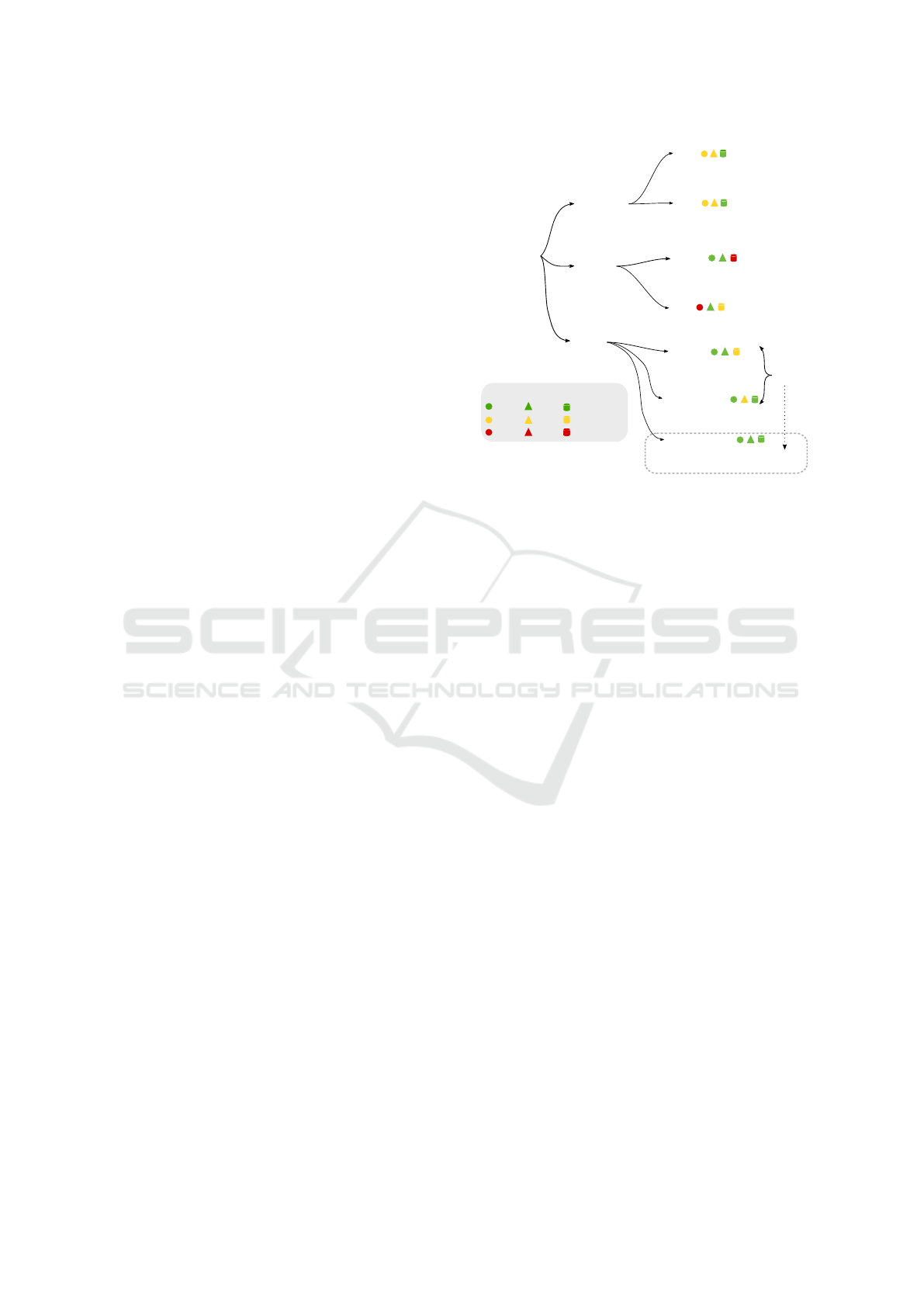
In this study, we build on a previously proposed CL
approach that utilizes two ANNs (Ans and Rousset,
1997). Figure 2 illustrates the two ANNs and the
two learning phases of this approach. During the first
learning phase 1 , the knowledge from the first ANN,
named Net 1, is “transferred” to the second ANN,
named Net 2, through pseudo-samples. That is, Net 2
is trained with the knowledge of Net 1, Net 1 being
the model used to generate a pseudo-dataset that rep-
resents the knowledge we want to transfer. As both
ANNs are identical, we use a simpler way than the
one proposed in (Ans and Rousset, 1997) to trans-
fer the knowledge. We duplicate the parameters of
Net 1 into Net 2 instead of using pseudo-samples in
the phase 1 . During the second learning phase 2 ,
new classes have to be integrated without degrad-
ing previously learned knowledge. Net 1 learns the
new classes, but also the pseudo dataset generated by
Net 2. In this section, we present the ANN architec-
ture employed in the dual-memory system of Figure
2, the sampling procedure used to generate pseudo-
data and the knowledge transfer procedure that em-
ploys distillation to transfer the knowledge from one
ANN to another. The incremental learning procedure
is explained in the next Section.
Figure 2: Dual-memory system. Knowledge transfer: Net 2
acquires Net 1 knowledge by learning the pseudo-samples
generated by Net 1. Consolidation: Net 1 searches for a pa-
rameter set for new tasks and old tasks by replaying pseudo-
samples from the previously learned tasks.
ICAART 2021 - 13th International Conference on Agents and Artificial Intelligence
208
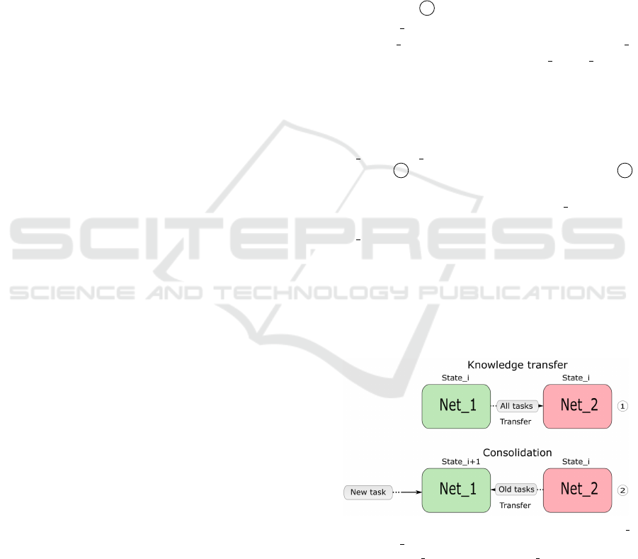
Figure 3: Auto-Hetero associative architecture.
3.1 The Auto-Hetero Associative
Architecture
Since the dual-memory system described above con-
sists of two identical ANNs, the description that fol-
lows is of only one ANN. The employed hybrid archi-
tecture is called Auto-Hetero (AH) associative ANN
because it is trained with a two-fold aim: replica-
tion and classification. The first aim is referred to as
“replication”, where for an input x
i
, the goal is to out-
put a ˆx
i
as close as possible to the input x
i
. The second
aim is referred to as “classification”, where for the in-
put x
i
, the goal is to output a label ˆy
i
as close as pos-
sible to the ground-truth label y
i
. Let us note that for
a dataset D with C classes, x
i
represents the ith sam-
ple and y
i
represents the ith label. The ground-truth
label y
i
is a one-hot C-dimensional vector and ˆy
i
is
a C-dimensional vector, whose values are in between
0 and 1. The samples x
i
and ˆx
i
are F-dimensional
vectors also in between 0 and 1. We employ the no-
tation [., .] to refer to the concatenation of two vec-
tors. For example, [x
i
,y
i
] is the P-dimensional vector
(P = F +C) that concatenates the F-dimensional vec-
tor x
i
and the C-dimensional vector y
i
.
The architecture of the AH associative ANN com-
prises an input layer which receives inputs x
i
, a cer-
tain number of hidden layers which transform x
i
from
the input layer and an output sigmoid layer. The out-
put sigmoid layer deliver the P-dimensional vector
([x
i
,y
i
]). An example of our AH associative ANN ar-
chitecture is presented in Figure 3.1. The proposed ar-
chitecture fulfills three main procedures: the training,
the inference and the generation of pseudo-samples.
The first procedure, the training, is performed by
minimizing the binary cross-entropy loss between the
output of the AH network [ ˆx
i
, ˆy
i
] and the ground-truth
outputs [x
i
,y
i
] using gradient descent. Equation (1)
defines this binary cross-entropy loss.
`
total
= −
∑
(x
i
,y
i
)∈D
h
P
∑
p=1
[x
i
,y
i
]
p
log([ ˆx
i
, ˆy
i
]
p
)
− (1 − [x
i
,y
i
]
p
)log(1 − [ ˆx
i
, ˆy
i
]
p
)
i
, (1)
where P is the dimension of the output of the neural
network, [x
i
,y
i
]
p
represents the pth element of the P-
dimensional vector [x
i
,y
i
] and [ ˆx
i
, ˆy
i
]
p
represents the
pth element of the P-dimensional vector [ˆx
i
, ˆy
i
].
In this way, the AH architecture is a hybrid model
that performs classification and replication. The sec-
ond procedure, the inference, employs the knowledge
gained during the training to infer the replication and
the label of a given input. While the auto-associative
output indicates how well the model is capable of re-
producing a given input, the hetero-associative output
indicates how well the model has built the decision
boundaries for classification. Finally, the generaliza-
tion ability of the model is always measured only by
taking into consideration the hetero-associative out-
put for the classification task. That is, the accuracy of
the model on the training and testing sets is computed
using the classification output. The third procedure,
the pseudo-sample generation procedure, is described
in the next subsection.
3.2 Reinjection Sampling Procedure
The pseudo-sample generation procedure, referred to
as reinjection (Ans and Rousset, 1997), employs the
Auto-associative component of the AH ANN to per-
form several inferences.
Figure 4: Reinjection sampling procedure.
The reinjection sampling procedure consists in cre-
ating a sequence of pseudo-samples with the auto-
associative output by following two steps: i. injecting
a random sample x
0
into the input layer of the auto-
associative component to infer its replication vector
x
1
; ii. reinjecting the replication vector x
1
in the in-
put layer to infer the next replication vector x
2
. The
process of bringing the replication vector in the in-
put layer is illustrated by the dot arrow in Figure 4
and it is referred to as reinjection. Therefore, a se-
quence of length one consists in ((x
0
) → [x
1
,y
0
]), a
sequence of length two consists in ((x
0
) → [x
1
,y
0
]
Beneficial Effect of Combined Replay for Continual Learning
209

; (x
1
) → [x
2
,y
1
]) and so on. Note that the hetero-
associative output provides only the label of each in-
put sample. For each reinjection, we gather three vec-
tors: the starting point, its corresponding label and
the replication of the starting point. The reinjection
sampling procedure mimics a non-conditional gener-
ative process where the samples are not conditioned
by the labels but by the starting point of the gener-
ated sequence. After each reinjection, the replica-
tion function corresponds, at first order, to a small
displacement towards higher densities in the train-
ing distribution (Bengio et al., 2013). Originally,
this procedure was implemented to generate pseudo-
samples that capture the knowledge of ANNs (Ans
and Rousset, 1997). In the original work, the authors
only take the last pseudo-sample of the generated se-
quence, which is the closest one to the learned distri-
bution concerning. In this work, we do not burn-in
(i.e discard iterations) the first samples of the begin-
ning of the sequence because the starting points are
samples from the tiny memory buffers instead of ran-
dom points. Thus, all the generated pseudo-samples
are gathered, hence generating the pseudo-sample se-
quence.
3.3 Knowledge Transfer
We employ the terminology introduced in (Hinton
et al., 2015), where the knowledge of a trained ANN
is defined by the mapping from input vectors to output
vectors. This abstract view of the knowledge is free
from any particular ANN implementation. In these
lines, a simple way to transfer the knowledge from a
trained ANN classifier to an untrained ANN classifier
is to employ the real samples and the so called soft
labels (logits), which are inferred by the trained ANN
classifier. The inferred labels, the soft labels, corre-
spond to the relative class probabilities delivered by
the trained classifier whereas the ground-truth labels
correspond to those given by the real dataset. For in-
stance, when an ANN classifier infers the soft label
of a sample, the classifier delivers probabilities for all
the classes. The information delivered by the proba-
bilities of all the classes is useful because a new clas-
sifier can build similar decision boundaries by learn-
ing the real samples and their corresponding soft la-
bels.
The latter knowledge transfer procedure is called
distillation and was originally proposed to transfer
the mapping function between different neural net-
works (Robins, 1995; Ans and Rousset, 1997; Hinton
et al., 2015). Distillation in CL is a common practice
that ensures that the information previously learned
is maintained during a new learning step. In com-
bined replay the set of generated inputs (x
i
) and out-
puts [x
i+1
,y
i
] defines the knowledge of a trained AH
ANN (see Figure 4). This knowledge is used to re-
duce forgetting when learning a new task as it is de-
scribed in the next Section.
4 COMBINED REPLAY
In the proposed combined replay method, Net 1
learns a new set of classes and its previous knowledge,
which is captured by Net 2 through reinjections, as
shown in Figure 5. Algorithm 1 lists the steps be-
hind combined replay (Figure 5). We consider that
“initially” Net 2 has already been trained on previ-
ous classes. The tiny memory buffer and the samples
of the new classes are provided. For each training
batch, we randomly draw samples from the tiny mem-
ory buffer D
old
and from the currently available train-
ing set D
new
1 and 3 respectively. Random noise is
added to the selected old samples (D
old
). The noisy
samples are reinjected several times to generate the
sequence of samples 2 . That is, Auto-Hetero (Net 2)
is evaluated in each reinjection for all the samples in
D
old
by delivering the “auto-hetero” output [x
i+1
,y
i
].
The soft-labeled pseudo-samples are merged with the
labeled real samples D
new
resulting in an enhanced
dataset 4 . Finally, the Auto-Hetero (Net 1) param-
eters are updated by minimizing the total loss `(θ
1
)
5 that encourages to learn the auto-hetero mapping
for the new set of classes and to consolidate the auto-
hetero output of the previously learned classes (distil-
lation loss). Net 2 retains the previous model param-
eters which are not updated during this phase. Note
that the distillation loss is the same loss formalized
above in Equation (1) but the pseudo-samples and
their inferred labels are employed instead of the true
samples and their corresponding ground-truth labels.
Basically, the workflow of Figure 5 is similar to
that in (Rebuffi et al., 2017) where a buffer and a
pre-updated classifier are used to perform distillation
to capture previous knowledge. There, the samples
of the buffer and their distilled outputs are jointly
learned with the new samples and their ground-truth
labels. Whereas the classification loss encourages the
classification of the newly observed classes, the dis-
tillation loss ensures that the previously learned infor-
mation is not lost. The differences here are the model
architecture and the way the buffer samples are used.
That is, we do no train a classifier; instead, we train an
Auto-Hetero associative ANN and perform reinjec-
tions to capture previous knowledge using the same
buffer.
In this way, during the consolidation step of Fig-
ICAART 2021 - 13th International Conference on Agents and Artificial Intelligence
210
Figure 5: Combined replay.
ure 2, two losses are employed to update the parame-
ters of Net 1 through backpropogation. The standard
classification and replication loss for the new sam-
ples (Equation (1)) encourages classifying and repli-
cating the new set of classes. The distillation loss
for the pseudo-samples and their corresponding soft-
labels (logits) ensures that the information previously
learned is not lost during the new learning stage.
5 EXPERIMENTS
This section describes the experiments carried out to
evaluate the performance of our approach against the
current state-of-the-art replay methods.
Baselines. We compare our method with the follow-
ing references:
• Auto-Hetero with buffer (AHB): An Auto-Hetero
model without reinjections, which is trained with
copied mini-batches of old samples (i.e. the old
samples and the corresponding labels) to reveal
whether the observed beneficial effects are due to
the hybrid architecture.
• Auto-Hetero with buffer noise (AHBN): An Auto-
Hetero model without reinjections, which is
trained with copied mini-batches of noised old
samples (i.e. the noised old samples and the cor-
responding ground-truth labels) to reveal if the
observed beneficial effects are due to the added
noise in the hybrid architecture. Note that AHBN
is very much akin to a denoising autoencoder im-
plementation with extra neurons for classification.
That is, the inputs are noised samples while the
Algorithm 1: Continual learning algorithm.
INPUT:
• x
s
,...,x
t
// training image of classes s,...,t
• noise strength // the strength of the noise added
before reinjections
• M // small memory buffer
• θ
1
// NET 1 model parameter
• θ
2
// NET
2 model parameter
• nb // number of learning steps
• R // number of reinjections
• lr // learning rate
for u = 0 to nb do
D
new
← ∪
y=s,...,t
{ (x
i
,y
i
) : x
i
∈ x
y
}
D
old
← ∪
y=1,...,s−1
{ (x
i
,·) : x
i
∈ x
y
}
D
old
= D
old
+ noise strength ∗ N (0, I)
X = [x
new
] (Samples)
XY = [(x
new
,y
new
)] (Samples for replication and
labels)
//reinjections
for e = 0 to R do
[x
n+1
,y
n
] ← AH(θ
2
,x
n
) for all (x
i
,·) ∈ D
old
// store pseudo-samples and their outputs
X = X ∪ [x
n
]
XY = XY ∪ [(x
n+1
,y
n
)]
end for
// run network training with total loss function
( eq.1 and distillation loss)
θ
1
← backprop(X, XY, θ
1
,lr)
end for
outputs are the true samples with the correspond-
ing ground-truth labels.
• ICARL (Classifier-based distillation): A rehearsal
method that saves a pre-updated version of a clas-
sifier to capture previous knowledge by employ-
ing a memory buffer. We implement the fully-
connected version of this method (Kemker and
Kanan, 2018), which employs two classifiers with
sigmoidal outputs and binary cross-entropy loss
for distillation. In the experiments, we take into
consideration this method due to its superior per-
formance at the same amount of available memory
compared to other CL methods (De Lange et al.,
2019).
• Episodic Replay (ER): A classifier that uses a
tiny memory buffer as a constraint to avoid catas-
trophic forgetting. It was recently stated that CNN
classifiers employing tiny memory buffers are less
prone to catastrophic forgetting than other popular
rehearsal methods (Chaudhry et al., 2019). In this
Beneficial Effect of Combined Replay for Continual Learning
211
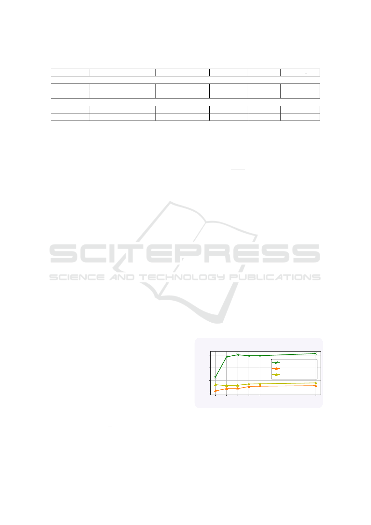
Table 1: Model Hyperparameters.
Models #units/hidden layer activation function epochs/class Optimizer learning rate
MNIST
Auto-Hetero [784,200,200,794] Mish 5 Adam 0.0001
Classifier [784,200,200,10] Mish 5 Adam 0.0001
CIFAR-10/100
Auto-Hetero [2048,1000,1000,2148] Mish 30 Adam 0.0001
Classifier [2048,1000,1000,100] Mish 2 Adam 0.001
work, a fully-connected version of this method is
implemented.
Datasets. We benchmark the beneficial effects of
reinjections on three commonly used datasets that dif-
fer in the number of classes and features. First, we
study the raw images from MNIST. Then, we extract
the features from CIFAR-10 and CIFAR-100 using a
resnet50 pre-trained on ImageNet (He et al., 2015).
The extracted features are also scaled between 0 and
1 using min-max normalization. It is worth noticing
that the maximum accuracy of a classifier trained on
the extracted features and their corresponding labels
of CIFAR-10 and CIFAR-100 datasets is around 92%
and 75% respectively.
The MNIST and CIFAR-10 benchmarks consist
of a total of 10 tasks where one task contains one
class. For CIFAR-100, we split the original CIFAR-
100 dataset into 20 disjoint subsets. Each subset is
considered as a separate task and contains 5 classes
from the total of 100 classes.
Let us note that T represents all the tasks to be
learned. In this context, a task refers to an isolated
training phase defined by (X
t
,Y
t
) such that X
t
is a set
of data samples for task t and Y
t
the corresponding
ground truth labels.
Metrics. The performance of all our experiments
are measured with a single-head evaluation metric.
That is, we do not use a task identifier; instead, we
identify the class to which a sample belongs accord-
ing to the classes learned so far independently. We
measure performance on the testing set using accu-
racy and forgetting, consistently with our domain’s
literature (Chaudhry et al., 2018a).
Accuracy: Let a
k, j
∈ [0, 1] be the accuracy (frac-
tion of correctly classified data from tasks 1 to k after
learning the task i). The higher the value of a
k
the bet-
ter the model performance on the classification task.
A
T
=
1
T
T
∑
j=1
a
T, j
(2)
Forgetting: Let f
i
∈ [−1, 1] be the forgetting on task i.
It measures the gap between the maximum accuracy
obtained in the past and the current accuracy about
the same task. The lower the forgetting, the better the
model performance.
F
T
=
1
T − 1
T −1
∑
j=1
(max
l∈1,...,i−1
a
l, j
) − a
i, j
(3)
Architectures. We perform all the experiments
with the baseline hyperparameters set presented in Ta-
ble 1 (see Table 1) for classifiers and for Auto-Hetero
ANNs, which we maintain constant to compare the
outcomes of the model under test. We employ the
Mish activation function for the hidden layer because
it has proved to be more robust than the relu activation
function for classification tasks (Misra, 2019). The
models are trained using the adam optimizer (Kingma
and Ba, 2014) with beta1=0.9 and beta2=0.5, and the
learning rates of Table 1. When learning CIFAR-
100 dataset, we only change two hyperparameters, the
epochs and the learning rate. This is due to the fact
that the AH architecture needs more learning steps
and a smaller learning rate to replicate and classify
CIFAR-100 correctly. The size of the mini-batch of
old and new samples is set to 10 irrespective of the
memory buffer size. The mini-batch of old samples is
copied as described below whenever reinjections are
performed.
0 1 2 3 4 9
0.5
0.6
0.7
0.8
Avg Accuracy
Combined
ICARL
ER
Replay
Reinjections/Copying
CIFAR-10
Figure 6: Final avg. accuracy of combined replay over rein-
jections/copying vs the final avg. accuracy of replay meth-
ods over the copied mini-batches for a memory buffer of
100 samples. The performance is averaged over 3 runs.
ICAART 2021 - 13th International Conference on Agents and Artificial Intelligence
212
10 50 100 150 200
0.2
0.4
0.6
0.8
Combined Replay
ICARL
AHB
AHBN
ER
Combined Replay
ICARL
AHB
AHBN
ER
Combined Replay
ICARL
AHB
AHBN
ER
1.0
Avg Accuracy
Avg Accuracy
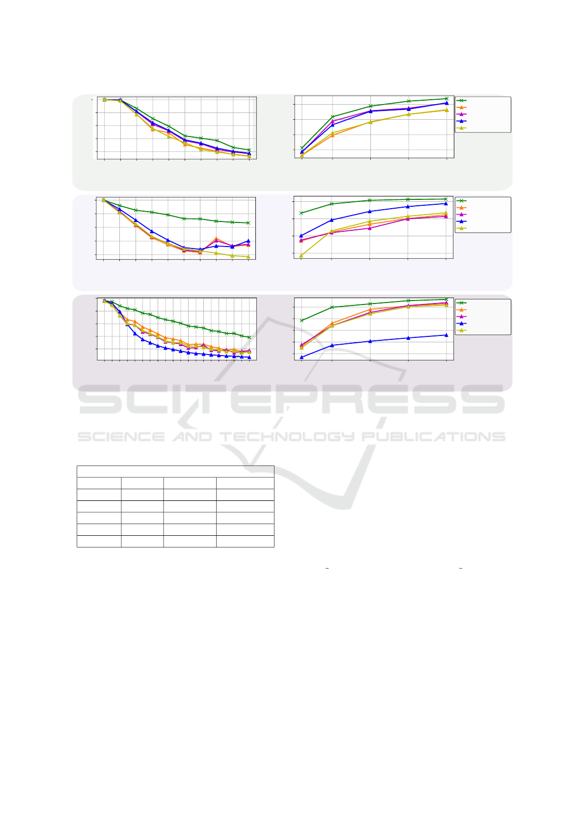
1 2 3 4 5 6 7 8 9 10
Tasks (1 class per tasks)
0.2
0.4
0.6
0.8
(a) MNIST
Avg Accuracy
10 50 100 150 200
0.2
0.4
0.6
0.8
1 2 3 4 5 6 7 8 9 10
Tasks (1 class per tasks)
0.2
0.4
0.6
0.8
1.0
Avg Accuracy
(b) CIFAR-10
(c) CIFAR-100
1 2 3 4 5 6 7 8 9 10 11 12 13 14 15 16 17 18 19 20
Tasks (5 classes per tasks)
0.2
0.4
0.6
0.8
1.0
Avg Accuracy
Avg Accuracy
100 500 1000 1500 2000
0.1
0.2
0.3
0.4
0.5
Memory buffer slots
Memory buffer slots
Memory buffer slots
Figure 7: On the left side, the average accuracy over tasks when only 1 sample per class is used. On the right side, the final
average accuracy as a function of the buffer size. The performance is averaged over 3 runs.
Table 2: Forgetting when using a tiny memory buffer of one
sample per dataset class taken . Forgetting is averaged over
3 runs.
Forgetting
Method MNIST CIFAR-10 CIFAR-100
CR(our) 0.7080 0.2603 0.3902
AHB 0.8137 0.4906 0.6957
AHBN 0.8044 0.5716 0.055
ICARL 0.8664 0.5040 0.7044
ER 0.8738 0.8664 0.7438
Methodology. We adapted the experimental setting
proposed in Experience Replay (Chaudhry et al.,
2019) (Alg. 1.) originally designed to benchmark
rehearsal methods. The original algorithm compares
the final performance of CL methods by carrying out
four main operations: i. the samples of the new set
of classes are learned only once. ii. the memory
buffer of old samples is updated at every learning step.
iii. the mini-batch of new classes (new samples) is
merged with the mini-batch of old classes (old sam-
ples) randomly selected from the memory buffer. iv.
the parameters of the models under test are updated by
backpropagating the loss of the merged mini-batches.
We made three adaptations to this algorithm:
• The new samples from the new set of classes are
learned several times.
• The memory buffer is updated after learning a
new task to ensure that it always contains only old
samples.
• The mini-batch of old samples is copied as many
times as reinjections are performed to update all
the methods with the same amount of old data.
In this way, after n reinjections, we obtain n∗mini-
batch size pseudo-samples. Mini-batch size refers to
the size of the mini-batch of old samples. To obtain
the same number of old true and pseudo-samples for a
fair comparison, we copied the true samples n times.
Therefore, if no reinjection is performed, no compen-
sation is needed – so the mini-batch is not copied. If
one reinjection is performed, the mini-batch of old
samples is duplicated to obtain the same mini-batch
size, and so on. Note that the interest behind copy-
ing the old mini-batches is to update all the rehearsal
methods with the equivalent amount of old data em-
ployed by combined replay.
Beneficial Effect of Combined Replay for Continual Learning
213
Results. In all our combined replay experiments,
we perform 4 reinjections; thus, the mini-batch is
quadrupled. Figure 6 shows the accuracy over the
number of reinjections and copied mini-batches on
CIFAR-10 dataset for a memory buffer size of 100
samples. In this way, we corroborate that the im-
pact of copying the mini-batches of old data does not
harm the generalization ability of the rehearsal meth-
ods. Furthermore, forgetting is not reduced and no
detriment is observed in the generalization ability.
We employed the reservoir sampling routine
(Chaudhry et al., 2019) to update the memory buffer
since any sample seen is equally likely to be stored.
We consider that the buffer size is bounded at (20 *
#classes). For instance, on CIFAR-100, the largest
buffer size is equal to 2000, which is also a size uti-
lized in the literature (Rebuffi et al., 2017; Castro
et al., 2018).
We average accuracy over 3 runs on test sets dur-
ing the learning steps. Figure 7 and Table 2 summa-
rize the results of the comparison with state of the art
approaches. The following observations can be made.
First, combined replay greatly outperforms all the
hybrid architectures that do not perform reinjections
(i.e. AHB and AHBN). Also, our approach outper-
forms state-of-the-art replay methods relying on the
same size of the memory buffers. Furthermore, for
very tiny memory buffers, combined replay yields a
higher performance at all benchmarks presented in
Figure 7. On CIFAR-100 (Figure 7(c)(right), for a
memory buffer of size 100, the accuracy of combined
replay is about 20% higher than EM and ICARL.
This result is interesting considering that the perfor-
mance of the CNN classifiers in ER seems to be
much higher than that of fully connected classifiers
(Chaudhry et al., 2019). We explain this result as fol-
lows: i. the test set is drawn from already seen ex-
amples of the training set in the original ER paper
(Chaudhry et al., 2019); ii. the CNN used for fea-
ture extraction might help retain previous knowledge
avoiding catastrophic forgetting. The difference in
performance between the methods gets smaller when
the memory buffer size becomes larger. For a mem-
ory buffer of 2000 samples (Figure 7(c)(right), the
curves meet by showing a comparable performance.
Moreover, ICARL delivers a slightly better perfor-
mance (52%) than that obtained in (Rebuffi et al.,
2017; Kemker and Kanan, 2018). This difference
might be due to the cloned mini-batches.
Second, it has already been observed that, often,
the reservoir sampling routine can completely dis-
lodge samples of the older classes when the memory
buffer is very small (Chaudhry et al., 2019). Even
though representative memory samples and balanced
training sets are not guaranteed with the reservoir up-
date routine, combined replay can capture a consid-
erable amount of knowledge from most previously
learned classes. The reinjections considerably allevi-
ate the lack of previous samples while other methods
experiment higher forgetting as it is shown in Table 2.
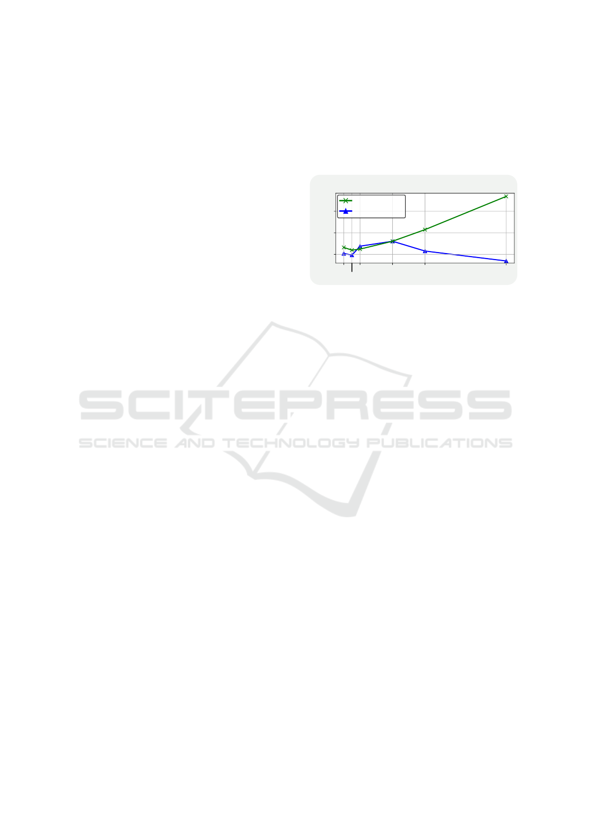
0.6
0.00
0.05
0.10 0.30 0.50
0.2
0.4
1.00
Noise
strength
Avg Accuracy
MNIST
AHBN
Combined
Replay
Figure 8: Final avg.accuracy of combined replay over noise
strength for a memory buffer of 10 samples. The perfor-
mance is averaged over 3 runs.
Third, the lowest value of forgetting for AHBN in Ta-
ble 2, on CIFAR-100 dataset, suggests that the denois-
ing implementation allows remembering some classes
quite well. However, the low values in the average ac-
curacy of Figure 7(left)(c) suggests that the denoising
implementation struggles to learn new tasks. Hence,
the forgetting and the accuracy results taken together
indicate that AHBN suffers from a lack of plasticity
(i.e. the inability to update its knowledge) after learn-
ing some tasks.
In summary, combined replay, employing reser-
voir sampling and very small memory buffers, out-
performs all the presented replay methods in terms
of accuracy and forgetting. For the selected hyper-
parameters (i.e. noise strength and number of rein-
jections), our solution shows a less pronounced slope
as the memory becomes larger. This suggests that
the knowledge captured through reinjections is mostly
beneficial when a reduced set of samples is available.
We observe that the knowledge captured with our ar-
chitecture reaches an optimal performance when a
memory buffer size of 10 samples per class is em-
ployed. While more knowledge can be captured using
larger memory buffers, the performance gain gradu-
ally decreases. This finding can be further confirmed
in Figure 7(c)(right) where ICARL, EM and our so-
lution yield similar performances when a memory
buffer of size 2000 is employed.
6 DISCUSSION
Combined replay highlights the importance of rein-
jections to improve the information retrieval process
ICAART 2021 - 13th International Conference on Agents and Artificial Intelligence
214

for transferring knowledge between two ANNs when
memory buffer sizes are constrained. Reinjections
are performed in a hybrid architecture to generate
pseudo-data that captures previously acquired knowl-
edge. The pseudo-data is generated with noised sam-
ples from tiny memory buffers through a reinjection
sampling procedure. When incrementally learning
new tasks, the pseudo-data set is jointly learned with
the samples of a new task to overcome catastrophic
forgetting. To further investigate combined replay, we
first analyze the memory footprint; second, the impact
of the added noise and, third, the number of reinjec-
tions performed.
First, in this work, we have prioritized the aver-
age accuracy regarding minimal memory buffer sizes;
however, for a final embedded implementation, we
could reduce the memory footprint by employing only
one AH model. In this way, the Net 2 in Figure 2
would no longer be required, and Net 1, which would
be the pre-updated model in the consolidation phase,
would be used only once to generate a pseudo-data set
capturing previously acquired knowledge.
Second, we investigate the quality of the pseudo-
data set in terms of the strength of added noise. Figure
8 presents the noise strength vs the average accuracy
for combined replay and AHBN. On MNIST dataset,
for a minimal memory buffer of size 10, the more
noise is added before performing reinjections, the bet-
ter combined replay captures previous knowledge. In
this case, the added noise can also improve the final
performance in AHBN as it is the case for a noise
strength between 0.1 and 0.3. However, a negative ef-
fect of noise in AHBN reveals that the performance
gain of combined replay is not due to a denoising ef-
fect but to reinjections. This finding suggests that a
careful optimization of this parameter would lead to
improved results; a study that is out of the scope of
the present paper. For simplicity, the combined re-
play employs an isotropic Gaussian noise N (0, I) that
is pondered by a noise strength of 0.05 in all experi-
ences of Figure 7 and Figure 6.
Third, the purpose of reinjections is to generate
a sequence of pseudo-samples to capture the knowl-
edge properly. All our experiments were performed
with four reinjections generating a pseudo-sample se-
quence of length five. In order to be fair, the mini-
batch of old samples are copied four times to update
all the rehearsal methods with the equivalent amount
of old data. We have empirically selected this number
so as not to harm the generalization ability of the clas-
sifiers in ICARL and ER. However, the knowledge
is well captured between 1 and 3 reinjections as it is
shown in Figure 6. Similar to the strength of the noise,
an optimized value of this parameter could lead to im-
proved results. As the knowledge captured through
reinjections tends to reach a limit at a certain point,
combined replay could end up being outperformed by
larger, better optimized memory buffers. However,
our approach shows a much higher efficiency when
the memory buffer size is limited, which is a crucial
constraint in many continual learning set-ups.
In a nutshell, the strength of the noise and the
number of reinjections play a crucial role in retrieving
previously acquired knowledge. These parameters di-
rectly regulate the generation of pseudo-samples that
influence the preservation of old knowledge. In our
view, these two parameters can be considered as a
function of the memory buffer size and the proper-
ties of the dataset (e.g. the distance between classes,
the number of samples per class, etc.). Forthcom-
ing research on combined replay could lead to im-
proved performances through selection of both the
noise strength and the number of reinjections.
7 CONCLUSION
This paper presents a novel approach for retrieving
previously learned information to reduce catastrophic
forgetting in artificial neural networks. The experi-
mental results on MNIST, CIFAR-10 and CIFAR-100
presented in the paper lead to the following conclu-
sions. First, our combined replay approach is more
robust than state-of-the-art replay methods when re-
lying on a minimal memory buffer. Second, our ap-
proach does not require representative memory sam-
ples and a balanced training sets to be efficient, two
mandatory conditions for other replay methods. Fu-
ture work will include the automatic determination of
noise strength and the number of reinjections to de-
liver improved results in embedded applications.
REFERENCES
Abraham, W. C. and Robins, A. (2005). Memory retention–
the synaptic stability versus plasticity dilemma.
Trends in neurosciences, 28(2):73–78.
Aljundi, R., Chakravarty, P., and Tuytelaars, T. (2017). Ex-
pert gate: Lifelong learning with a network of experts.
In Proceedings of the IEEE Conference on Computer
Vision and Pattern Recognition, pages 3366–3375.
Aljundi, R., Rohrbach, M., and Tuytelaars, T. (2018).
Selfless sequential learning. arXiv preprint
arXiv:1806.05421.
Ans, B. and Rousset, S. (1997). Avoiding catastrophic
forgetting by coupling two reverberating neural net-
works. Comptes Rendus de l’Acad
´
emie des Sciences-
Series III-Sciences de la Vie, 320(12):989–997.
Beneficial Effect of Combined Replay for Continual Learning
215

Atkinson, C., McCane, B., Szymanski, L., and Robins, A.
(2018). Pseudo-recursal: Solving the catastrophic
forgetting problem in deep neural networks. arXiv
preprint arXiv:1802.03875.
Bengio, Y., Yao, L., Alain, G., and Vincent, P. (2013). Gen-
eralized denoising auto-encoders as generative mod-
els. In Advances in neural information processing sys-
tems, pages 899–907.
Castro, F. M., Mar
´
ın-Jim
´
enez, M. J., Guil, N., Schmid, C.,
and Alahari, K. (2018). End-to-end incremental learn-
ing. In Proceedings of the European conference on
computer vision (ECCV), pages 233–248.
Chaudhry, A., Dokania, P. K., Ajanthan, T., and Torr, P. H.
(2018a). Riemannian walk for incremental learning:
Understanding forgetting and intransigence. In Pro-
ceedings of the European Conference on Computer
Vision (ECCV), pages 532–547.
Chaudhry, A., Ranzato, M., Rohrbach, M., and Elhoseiny,
M. (2018b). Efficient lifelong learning with a-gem.
arXiv preprint arXiv:1812.00420.
Chaudhry, A., Rohrbach, M., Elhoseiny, M., Ajanthan,
T., Dokania, P. K., Torr, P. H., and Ranzato, M.
(2019). On tiny episodic memories in continual learn-
ing. arXiv preprint arXiv:1902.10486.
De Lange, M., Aljundi, R., Masana, M., Parisot, S.,
Jia, X., Leonardis, A., Slabaugh, G., and Tuyte-
laars, T. (2019). A continual learning survey: Defy-
ing forgetting in classification tasks. arXiv preprint
arXiv:1909.08383.
Farquhar, S. and Gal, Y. (2018). Towards robust evalua-
tions of continual learning. Bayesian Deep Learning
Workshop at NeurIPS.
Fernando, C., Banarse, D., Blundell, C., Zwols, Y., Ha, D.,
Rusu, A. A., Pritzel, A., and Wierstra, D. (2017). Path-
net: Evolution channels gradient descent in super neu-
ral networks. arXiv preprint arXiv:1701.08734.
Goodfellow, I., Pouget-Abadie, J., Mirza, M., Xu, B.,
Warde-Farley, D., Ozair, S., Courville, A., and Ben-
gio, Y. (2014). Generative adversarial nets. In
Advances in neural information processing systems,
pages 2672–2680.
He, K., Zhang, X., Ren, S., and Sun, J. (2015). Deep resid-
ual learning for image recognition. arXiv preprint
arXiv:1512.03385.
Hinton, G., Vinyals, O., and Dean, J. (2015). Distilling the
knowledge in a neural network. NIPS Deep Learning
and Representation Learning Workshop.
Hocquet, G., Bichler, O., and Querlioz, D. (2020). Ova-inn:
Continual learning with invertible neural networks.
arXiv preprint arXiv:2006.13772.
Jeon, I. and Shin, S. (2019). Continual representa-
tion learning for images with variational continual
auto-encoder. In Proceedings of the 11th Interna-
tional Conference on Agents and Artificial Intelli-
gence - Volume 2: ICAART,, pages 367–373. IN-
STICC, SciTePress.
Kemker, R. and Kanan, C. (2018). Fearnet: Brain-inspired
model for incremental learning. International Confer-
ence on Learning Representations (ICLR).
Kingma, D. P. and Ba, J. (2014). Adam: A method for
stochastic optimization. 3rd International Conference
on Learning Representations ICLR.
Kingma, D. P. and Welling, M. (2014). Auto-encoding vari-
ational bayes. International Conference on Learning
Representations (ICLR).
Kirkpatrick, J., Pascanu, R., Rabinowitz, N., Veness, J.,
Desjardins, G., Rusu, A. A., Milan, K., Quan, J.,
Ramalho, T., Grabska-Barwinska, A., et al. (2017).
Overcoming catastrophic forgetting in neural net-
works. Proceedings of the national academy of sci-
ences, 114(13):3521–3526.
Krizhevsky, A., Hinton, G., et al. (2009). Learning multiple
layers of features from tiny images.
Lavda, F., Ramapuram, J., Gregorova, M., and Kalousis, A.
(2018). Continual classification learning using gener-
ative models. arXiv preprint arXiv:1810.10612.
LeCun, Y., Cortes, C., and Burges, C. (2010). Mnist hand-
written digit database. ATT Labs [Online]. Available:
http://yann.lecun.com/exdb/mnist, 2.
Lesort, T., Gepperth, A., Stoian, A., and Filliat, D. (2019).
Marginal replay vs conditional replay for continual
learning. In International Conference on Artificial
Neural Networks, pages 466–480. Springer.
Mallya, A. and Lazebnik, S. (2018). Packnet: Adding mul-
tiple tasks to a single network by iterative pruning. In
Proceedings of the IEEE Conference on Computer Vi-
sion and Pattern Recognition, pages 7765–7773.
McCloskey, M. and Cohen, N. J. (1989). Catastrophic in-
terference in connectionist networks: The sequential
learning problem. In Psychology of learning and mo-
tivation, volume 24, pages 109–165. Elsevier.
Misra, D. (2019). Mish: A self regularized non-
monotonic neural activation function. arXiv preprint
arXiv:1908.08681.
Parisi, G. I., Kemker, R., Part, J. L., Kanan, C., and
Wermter, S. (2019). Continual lifelong learning with
neural networks: A review. Neural Networks, 113:54–
71.
Prabhu, A., Torr, P., and Dokania, P. (2020). Gdumb: A
simple approach that questions our progress in contin-
ual learning. In The European Conference on Com-
puter Vision (ECCV).
Rannen, A., Aljundi, R., Blaschko, M. B., and Tuytelaars,
T. (2017). Encoder based lifelong learning. In Pro-
ceedings of the IEEE International Conference on
Computer Vision, pages 1320–1328.
Rebuffi, S.-A., Kolesnikov, A., Sperl, G., and Lampert,
C. H. (2017). icarl: Incremental classifier and rep-
resentation learning. In Proceedings of the IEEE con-
ference on Computer Vision and Pattern Recognition,
pages 2001–2010.
Robins, A. (1995). Catastrophic forgetting, rehearsal and
pseudorehearsal. Connection Science, 7(2):123–146.
Rusu, A. A., Rabinowitz, N. C., Desjardins, G., Soyer,
H., Kirkpatrick, J., Kavukcuoglu, K., Pascanu, R.,
and Hadsell, R. (2016). Progressive neural networks.
arXiv preprint arXiv:1606.04671.
Shin, H., Lee, J. K., Kim, J., and Kim, J. (2017). Continual
learning with deep generative replay. In Advances in
Neural Information Processing Systems, pages 2990–
2999.
ICAART 2021 - 13th International Conference on Agents and Artificial Intelligence
216

Wu, C., Herranz, L., Liu, X., van de Weijer, J., Radu-
canu, B., et al. (2018). Memory replay gans: Learn-
ing to generate new categories without forgetting. In
Advances in Neural Information Processing Systems,
pages 5962–5972.
Xu, J. and Zhu, Z. (2018). Reinforced continual learning. In
Advances in Neural Information Processing Systems,
pages 899–908.
Zenke, F., Poole, B., and Ganguli, S. (2017). Continual
learning through synaptic intelligence. Proceedings
of machine learning research, 70:3987.
Beneficial Effect of Combined Replay for Continual Learning
217
