A New Generic Progressive Approach based on Spectral Difference for
Single-sensor Multispectral Imaging System
Vishwas Rathi
1 a
, Medha Gupta
2 b
and Puneet Goyal
1 c
1
Department of Computer Science and Engineering, Indian Institute of Technology Ropar, Rupnagar, Punjab, India
2
Department of Computer Science and Engineering, Graphic Era University, Dehradun, India
Keywords:
Multispectral Imaging System, Image Demosaicking, Multispectral Filter Array, Color Difference,
Interpolation, Spectral Correlation.
Abstract:
Single-sensor RGB cameras use a color filter array to capture the initial image and demosaicking technique
to reproduce a full-color image. A similar concept can be extended from the color filter array (CFA) to a
multispectral filter array (MSFA). It allows us to capture a multispectral image using a single-sensor at a low
cost using MSFA demosaicking. The binary tree based MSFAs can be designed for any k-band multispectral
images and are preferred, however the existing demosaicking methods are either not generic or are of limited
efficacy. In this paper, we propose a new generic demosaicking method applicable on any k-band MSFAs,
designed using preferred binary-tree based approach. The proposed method involves applying the bilinear
interpolation and estimating the spectral correlation differences appropriately and progressively. Experimen-
tal results on two different multispectral image datasets consistently show that our method outperforms the
existing state-of-art methods, both visually and quantitatively, as per the different metrics.
1 INTRODUCTION
The energy transmitted from light origins or reflected
by objects contains a wide range of wavelengths. The
standard color image contains the scene’s information
in only three bands: Red, Green and Blue. How-
ever, a multispectral image has more than three spec-
tral bands, which makes the multispectral image more
informative about the scene than the standard color
image. Therefore, multispectral images are found
useful in many research areas such as remote sens-
ing (MacLachlan et al., 2017), medical imaging (Zen-
teno et al., 2019), food industry (Qin et al., 2013;
Chen and Lin, 2020), satellite imaging (Mangai et al.,
2010) and computer vision (Ohsawa et al., 2004;
Vayssade et al., 2020; Junior et al., 2019). Depending
on the application, there are different requirements of
information captured through multiple spectral bands.
These multiple requirements in different domains mo-
tivated the manufacturer to develop different multi-
spectral imaging (MSI) systems (Fukuda et al., 2005;
Thomas et al., 2016; Geelen et al., 2014; Pichette
a
https://orcid.org/0000-0002-6770-6142
b
https://orcid.org/0000-0001-6013-3719
c
https://orcid.org/0000-0002-6196-9347
1 5 2 5
4 3 4 3
2 1 5
3434
5
1 7 2 8
5 3 6 4
2 1 7
3546
8
1 13 4 15
9 5 11 7
3 2 14
610812
15
1 11 4 12
9 5 10 7
3 2 11
69810
12
1 2 3 54
1 2 3
5 6 7
4
8
12
4321
5 6 7 8
9 10 11
1 2 3 4 5
6 7 8 9 10
11 12 13 14 15
5 Band
8 Band
12 Band 15 Band
(a)
(b)
5 Band 8 Band 12 Band 15 Band
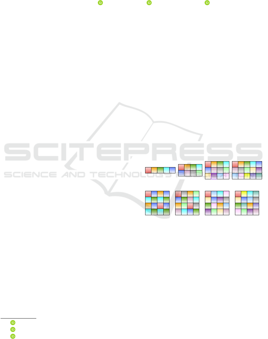
Figure 1: MSFA designs. (a) Non-redundant MSFAs used
in (Brauers and Aach, 2006; Gupta and Ram, 2019). (b)
Binary-tree based MSFAs defined in (Miao and Qi, 2006).
et al., 2016; Ohsawa et al., 2004; Monno et al., 2015)
of varying bands.
The concept of the single-camera-one-shot system
is recently getting explored to develop low-cost mul-
tispectral imaging systems using the MSFA similar to
the standard color camera that also uses a single sen-
sor to capture three bands’ information with a CFA.
The image captured using a single-camera-one-shot
system records only one spectral band information at
each pixel location and this image is called a mo-
saic image or MSFA image in the multispectral do-
main. A complete multispectral image is generated
Rathi, V., Gupta, M. and Goyal, P.
A New Generic Progressive Approach based on Spectral Difference for Single-sensor Multispectral Imaging System.
DOI: 10.5220/0010250103290336
In Proceedings of the 16th International Joint Conference on Computer Vision, Imaging and Computer Graphics Theory and Applications (VISIGRAPP 2021) - Volume 4: VISAPP, pages
329-336
ISBN: 978-989-758-488-6
Copyright
c
2021 by SCITEPRESS – Science and Technology Publications, Lda. All rights reserved
329

from an MSFA image using an interpolation method
called MSFA demosaicking. This single-sensor mul-
tispectral imaging system (SSMIS) would be of low
cost and small size, and can also capture videos in the
multispectral domain.
However, MSFA demosaicking is a challenging
task because of the highly sparse sampling of each
spectral band. As the number of spectral bands in a
multispectral image increases, the spatial correlation
is lower in the image. That is why SSMIS consider-
ing only spatial correlation does not perform well on
higher spectral bands multispectral images. Further,
the quality of the multispectral image generated us-
ing SSMIS depends on the demosaicking method and
the MSFA pattern used to capture the mosaic image.
As there is no such de-facto standardfor MSFA de-
sign similar to the Bayer pattern in the RGB domain,
the MSFA pattern choice becomes crucial.The binary
tree based MSFAs that can be designed for any k-band
multispectral images, are preferred (Miao and Qi,
2006; Gupta and Ram, 2019). Also, as the require-
ment of the number of spectral bands is application-
specific, it motivates the need for development of a
generic MSFA demosaicking method for wider appli-
cability. This research, therefore, aims to develop a
generic MSFA demosaicking method for SSMIS us-
ing binary tree based MSFAs to provide better qual-
ity multispectral images. The existing generic MSFA
demosaicking methods (Miao et al., 2006; Brauers
and Aach, 2006) fail to generate good quality multi-
spectral images, especially for higher band multispec-
tral images. The other MSFA demosaicking methods
(Mihoubi et al., 2017; Monno et al., 2015; Monno
et al., 2012; Monno et al., 2011; Jaiswal et al., 2017)
are restricted to multispectral images of some specific
band size.
This paper proposes an MSFA demosaicking
method utilizing both the spatial and spectral corre-
lation in the MSFA image. The proposed method is
generic, i.e., not restricted for any specific number of
spectral band images. It uses the binary-tree based
MSFA patterns (Miao and Qi, 2006), which are con-
sidered most compact and designable for any num-
ber of bands. The proposed method first interpolates
the missing pixel by performing progressive bilin-
ear interpolation, explicitly designed for binary-tree
based MSFA pattern. Then these interpolated bands
are used progressively in the spectral correlation dif-
ference method. Experimental results on multiple
benchmark datasets show that the proposed method
outperforms other state-of-the-art generic MSFA de-
mosaicking methods, both visually and quantitatively.
2 RELATED WORK
In this section, we discuss different MSFA patterns
present in the literature and associated MSFA demo-
saicking methods.
2.1 Different MSFA Patterns
We divide the MSFA patterns into two categories, as
shown in Figure 1, depending on the probability of
appearance(PoA) of bands in the MSFA pattern.
1. There are many MSFA designs (Brauers and
Aach, 2006; Mihoubi et al., 2015; Aggarwal
and Majumdar, 2014) where each band has
equal PoA in the MSFA pattern. Brauers and
Aach (Brauers and Aach, 2006) proposed a six-
band non-redundant MSFA pattern which stores
bands in 3×2 matrix. This was later extended and
the generalized designs for non-redundant MSFA
patterns were presented (Gupta and Ram, 2019).
Also, Aggarwal and Majumdar (Aggarwal and
Majumdar, 2014) proposed uniform and random
MSFA pattern design; both of these are generic
and can be extended to capture any number of
bands multispectral images. Mihoubi et. al. (Mi-
houbi et al., 2015) used square non-redundant
MSFA design for the 4, 9, and 16-band images.
2. Another category of MSFA design is binary-tree
based where MSFA is more compact and the sev-
eral spectral bands can have different PoA in the
MSFA pattern. Miao and Qi (Miao and Qi, 2006)
proposed this binary-tree based generic method to
generate MSFA patterns using a binary tree for
any number of bands multispectral images. These
are more preferred compared to redundant ones
and many of the recent works have used binary-
tree based MSFAs (Miao and Qi, 2006). Monno
et al. in his works (Monno et al., 2012; Monno
et al., 2011; Monno et al., 2014; Monno et al.,
2015) used five-band MSFA pattern where, PoA
of G-band is kept 0.5.
2.2 MSFA Demosaicking
The method (Brauers and Aach, 2006) extended the
color-difference-interpolation of CFA demosaicking
to the multispectral domain. But it failed to gener-
ate quality multispectral images. Further, (Mizutani
et al., 2014) improved Brauers and Aach method by
iterating demosaicking methods multiple times. The
number of iterations depended on the correlation be-
tween two spectral bands.
Miao et al. (Miao et al., 2006) proposed a binary
tree-based edge sensing (BTES) generic method for
VISAPP 2021 - 16th International Conference on Computer Vision Theory and Applications
330
MSFA demosaicking that used the MSFA patterns
generated using (Miao and Qi, 2006). BTES method
used the same binary tree for interpolation, which is
used to design MSFA pattern. BTES performed edge
sensing interpolation to develop a complete multi-
spectral image. Although BTES is generic, it does not
perform well on a higher band multispectral image as
it uses only spatial correlation.
In (Aggarwal and Majumdar, 2014), authors used
uniform MSFA design for MSFA demosaicking and
proposed a linear demosaicking method that requires
the prior computation of parameters using original
images. This limits the feasibility and applicability of
the method as original images would not be available
in real-time situation. Mihoubi et. al. (Mihoubi et al.,
2015) used the concept of intensity image, which has
a strong spatial correlation with each band than bands
considered pairwise. Further, Mihoubi et al. in (Mi-
houbi et al., 2017) had improved their previous work
by proposing a new estimation of intensity image.
However, their method is not generic.
Monno et. al. (Monno et al., 2015; Monno et al.,
2012; Monno et al., 2011; Monno et al., 2014) pro-
posed several methods considering the MSFAs de-
signed using the binary-tree based method and used
the concept of guide image which was generated from
under sampled G-band, and later they used this guide
image as a reference to interpolate remaining under-
sampled bands. (Monno et al., 2011) extended exist-
ing upsampling methods to adaptive kernel upsam-
pling methods using an adaptive kernel to reconstruct
each band and later improved in (Monno et al., 2012)
using the guided filter. To further improve (Monno
et al., 2012), in (Monno et al., 2015), the authors con-
structed multiple guide images and used them for in-
terpolation. This approach is not effective for a higher
band multispectral image. It is limited to the MSFA
pattern where G-band has PoA 0.5, making other
bands severely undersampled in higher band multi-
spectral image. (Jaiswal et al., 2017) also utilized the
MSFA generated using (Monno et al., 2015). Here,
authors proposed a method using frequency domain
analysis of spectral correlation for five-band multi-
spectral images. This method requires the complete
information of multispectral images for the model’s
learning parameters estimation, which would not be
available in real practice for MSFA based multispec-
tral camera device intended to be developed.
Few machine learning and deep learning-based
MSFA demosaicking methods (Aggarwal and Ma-
jumdar, 2014; Shopovska et al., 2018; Habtegebrial
et al., 2019) also has been recently explored. How-
ever, these methods require atleast some of the origi-
nal multispectral images of the SSMIS for the learn-
PBSD
MSFA Image
PB
EstimatedImage
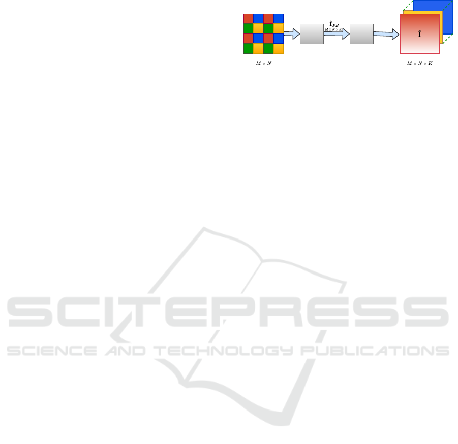
Figure 2: Proposed MSFA demosaicking approach.
ing and training of model parameters, but that will
not be available in the real world capturing scenario
for the considered SSMIS.
3 PROPOSED METHODOLOGY
In this paper, we propose an MSFA demosaicking
method that is based on progressive bilinear interpo-
lation and progressive bilinear spectral difference. As
shown in Figure 2, the complete method essentially
comprises of two steps, mentioned as follows:
1. First, interpolate the missing pixel values using
a progressive bilinear (PB) approach designed
specifically for the binary tree based MSFA pat-
terns.
2. Second, use progressive bilinear spectral differ-
ence (PBSD) approach based on inter-band dif-
ferences and applied progressively.
In the following subsections 3.1 and 3.2, we present
these steps in more details.
3.1 Progressive Bilinear (PB)
Interpolation
Here, we describe a new intra-band progressive ap-
proach for estimating the missing pixel values at a few
unknown locations using the bilinear interpolation on
some initially known pixel values, as per the binary-
tree based MSFA and the specific spectral band con-
sidered. Then, these estimated pixel values with ini-
tially known pixel values are used to calculate miss-
ing pixel values at other locations. PB interpolation
approach consists of the following components.
3.1.1 Pixel Selection
PB interpolation is an intra-band approach and thus
independent of the order of bands selected for the in-
terpolation. But the order of pixel locations chosen
for the interpolation for the different bands is differ-
ent. This pixel selection order critically depends on
the binary tree used to create the MSFA pattern, de-
signed using (Miao and Qi, 2006). For any chosen
A New Generic Progressive Approach based on Spectral Difference for Single-sensor Multispectral Imaging System
331
1 2
i
ii
3
r
4 5
iii
1 5 2 5
4 3 4 3
2 1 5
3434
5
1
1
5 2 5
4
2
4
1
5
5
5
4 43 3
3
3
4 3
2
2
2 2
4
4
1
1 1
4
5 5 5
4 4
5
3
3
3
5
5
5
33 34 4
(b)
3
(a)
1
1
1
1
1
1
1 1
(c)
1 1
1 1
1 1
11
1
1
1
1
1
1 1
1
1
1
1
1
1 1
1
1 1
1
1
1
1
11 1
(e)
1 1 1 1
1 1 1 1
1 1 1
1111
1
1
1
1 1 1
1
1
1
1
1
1
1
1 11 1
1
1
1 1
1
1
1 1
1
1
1
1 1
1
1 1 1
1 11
1
1
1
1
1
1
1
11 11 1
(f)
1 1
1 1
1
1
1
1
1
1
1
1 1
1
1 1
(d)
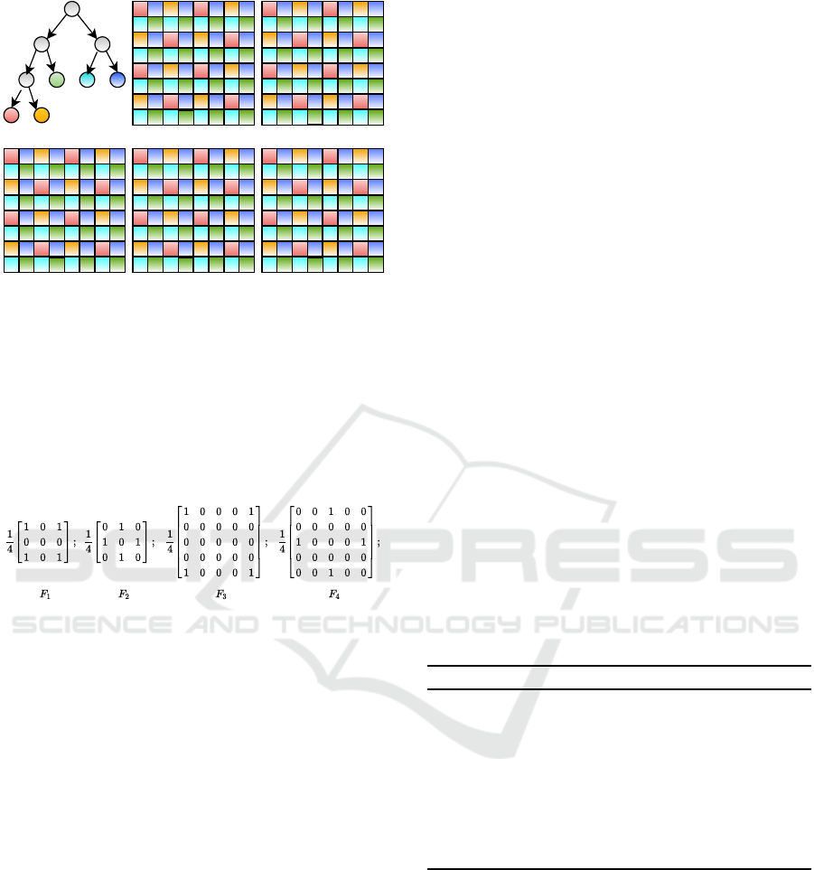
Figure 3: Illustration of PB interpolation of band 1. (a) Bi-
nary tree used to generate 5-band MSFA. (b) 5-band MSFA
pattern for 8×8 size mosaic (raw) image. (c) Band 1’s pixel
locations in the original mosaic image; one may note that
band 1’s PoA = 1/8 initially. (d) Band 1 estimated first at
the locations of a band corresponding to sibling node, i.e.,
band 2, using filter F
4
. (PoA now = 1/4) (e) Later, interpo-
late at the locations of band 3 using filter F
1
(Band 1 PoA
now = 1/2) (f) Finally, interpolate at the locations of band 4
and 5 using filter F
2
.
Figure 4: Filters used for PB interpolation.
band during interpolation, we first estimate the miss-
ing band information at the sibling band’s pixel lo-
cations and move one level up in the binary tree and
repeat the same process until we estimate the missing
band information at all locations. If the sibling node
is an internal node, then the bands corresponding to
the leaves under the sibling node can be considered
in any order. For example, consider the binary tree
for a 5-band multispectral image and corresponding
MSFA pattern-based mosaic image, as shown in Fig-
ure 3(a) and (b), respectively. For interpolating band
1, we can select the pixel locations either in the or-
der: {2,3,4,5} or {2,3,5,4}. For interpolating band 3,
we can select the pixel locations either in the order:
{1,2,4,5}, {2,1,4,5} {1,2,5,4} or {2,1,5,4}, and for
interpolating band 4, we must first select pixel loca-
tions corresponding to band 5 and then locations for
the other bands 1, 2 and 3 in any order.
3.1.2 Interpolation
Given the pixel selection order for a band, the miss-
ing pixel values of this band are progressively in-
terpolated using the four closest known neighboring
pixel values of the same band. This closest neighbor-
hood, at any progressive step, depends on the PoA of
the known (original and/or estimated) pixel values of
the selected band. For the binary-tree based MSFA
patterns, it can be observed that the 3 × 3 neighbor-
hood of a missing data pixel will contain at least four
known pixels if PoA of the band considered is greater
than or equal to 1/4, and for the band pixels with PoA
less than 1/4 but greater than or equal to 1/16, four
known neighboring pixels will lie in 5 × 5 neighbor-
hood. Based on the locations of the known neighbor-
ing pixels in the closest neighborhood, we select the
filter and perform convolution at pixel locations of the
selected band in the pixel selection scheme. The fil-
ters are shown in Figure 4, and can work up to 16
bands multispectral image. In Algo. 1, we define
the interpolation scheme, which interpolates band q
at other band locations. The same algorithm can be
repeated to interpolate all the bands of the multispec-
tral image. In Figure 3(c), to interpolate band 1 at
some location (i,j) of band 2, four nearest pixel val-
ues of band 1 are found in 5 × 5 neighborhood at lo-
cations (i-2,j), (i+2,j), (i,j-2), and (i,j+2). Therefore,
F4 filter is used to interpolate band 1 at locations of
band 2. After interpolating at band 2 locations, PoA
of band 1 increases to 1/4, as shown in Figure 3(d),
which makes four nearest pixel values of band 1 to be
available in 3 × 3 neighborhood. Further, to interpo-
late band 1 at locations of band 3, we use filter F
1
and
finally, we use filter F
2
to interpolate at band 4 and 5
locations.
Algorithm 1: Interpolation scheme for band-q.
Input: I
MSFA
,F, M
B
,q
1
˜
I
q
= I
MSFA
m
q
// Initialization
2 For each band p taken in the order given by
pixel selection scheme, repeat following
steps 3 and 4;
3 Select F
i
based on current PoA of
˜
I
q
4
˜
I
q
=
˜
I
q
+
˜
I
q
∗ F
i
m
p
5
ˆ
I
q
PB
=
˜
I
q
where, I
MSFA
is K band mosaic image of size M ×
N, F = {F
1
,F
2
,F
3
,F
4
} is set of filters used, M
B
=
{m
1
,...m
K
} is set of K binary masks, each of size
M × N, ’∗’ is convolution operator, and ’’ is ele-
ment wise multiplication operator. The binary mask
m
q
has value 1 only at locations where q
th
band’s orig-
inal values are there.
VISAPP 2021 - 16th International Conference on Computer Vision Theory and Applications
332

3.2 Progressive Bilinear Spectral
Difference (PBSD)
The PBSD method is applicable for any binary-tree
based MSFAs and thus it can be used to interpo-
late any K-band images using PB interpolation. It
is motivated from color difference based interpola-
tion method (Brauers and Aach, 2006). Using
ˆ
I
PB
as
the initial multispectral image, the following steps are
performed to generate the interpolated
ˆ
I multispectral
image.
1. For each ordered pair (p,q) of bands, determine
the sparse band difference
˜
D
pq
at q
th
band’s loca-
tions.
˜
I
q
= I
MSFA
m
q
(1)
˜
D
pq
=
ˆ
I
p
PB
m
q
−
˜
I
q
(2)
2. Now compute the fully-defined band difference
ˆ
D
pq
using PB interpolation of
˜
D
pq
. Computing
this on binary tree based MSFAs is feasible only
because of the new approach i.e. PB, as described
in subsection 3.1.
3. For each band q, estimate
ˆ
I
q
at pixel locations
where m
p
(x,y) = 1 as:
ˆ
I
q
=
K
∑
p=1
˜
I
p
−
ˆ
D
pq
m
p
(3)
Now, all K bands are fully-defined and together form
the complete multispectral image
ˆ
I.
4 EXPERIMENTAL RESULTS
We implement the proposed method PBSD and ex-
amine its performance on two publicly available mul-
tispectral image datasets: (a) Cave dataset (Yasuma
et al., 2010) and (b) TokyoTech dataset (Monno et al.,
2015). The Cave dataset contains 31 images each of
having 31-bands, and these bands range from 400nm
to 700nm with a spectral gap of 10nm. The Toky-
oTech dataset contains 30 images. Each image has
31-bands, and the spectral range of these 31-bands is
from 420nm to 720nm with a spectral gap of 10nm.
We consider multispectral images with band size (K)
varying from 5 to 15. The K-band multispectral im-
ages were prepared from these 31-band images by se-
lecting K-bands at equal spectral gaps beginning from
the first band. We obtain the mosaic image by sam-
pling the pixel values based on the MSFA pattern de-
fined for each band and then applying the MSFA de-
mosaicking method to estimate the complete multi-
spectral image.
We compare the proposed method with other
existing generic MSFA demosaicking methods:
WB (Gupta and Ram, 2019), SD (Brauers and Aach,
2006), LMSD (Aggarwal and Majumdar, 2014),
ISD (Mizutani et al., 2014), IID (Mihoubi et al.,
2015), and BTES (Miao et al., 2006). We consider
CIE D65 illumination for the evaluation of methods.
To compare the estimated image’s quality with the
original image, we evaluate these methods based on
the PSNR and SSIM image quality metrics.
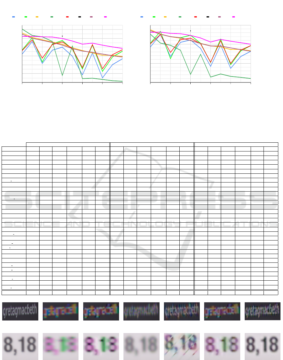
Figure 5 represents the quantitative performance
of different methods. For many larger bands images,
the SD and ISD methods seem to perform better than
the BTES method. However, the BTES method, using
compact (binary-tree based) MSFAs, performs better
for some bands such as 5, 7, 11, and 13. The sharp de-
crease in the performance for the 5, 7, 11, and 13 band
images in WB, SD, and ISD methods is because of
the non-compact characteristics of the non-redundant
MSFAs used in these methods. This observation was
the motivation for the proposed method. For seven
and higher bands multispectral image, the proposed
method PBSD performs consistently better than the
other methods, including BTES and LMSD, on both
datasets considered. This may be noted that the
IID method is applicable only to the non-redundant
MSFA pattern of square size (e.g. 2×2, 3×3, or 4×4).
Thus its results are shown here in Figure 5 for only 9-
band multispectral images.
Tables 1 and 2 represent reconstruction results for
8, 11 and 14 band multispectral images using differ-
ent MSFA demosaicking methods. It can be observed
that the proposed method PBSD performing better
and provides 1-2 dB average PSNR improvement in
compared to second best performing method. Table
3 shows the overall average PSNR and SSIM values
taken over different bands (5-band to 15-band) multi-
spectral images. The existing method BTES performs
reasonably better than other existing methods, how-
ever the proposed method PBSD performs the best by
providing further improvement of 1.25 dB in PSNR
and around 0.9% in SSIM on BTES on the Cave
dataset and 1.21 dB in PSNR and 2.5% in SSIM on
the TokyoTech dataset images.
Figure 6 shows the visual comparison of the few
images from the Cave and TokyoTech datasets gen-
erated by the various MSFA demosaicking methods
for 7 and 14 band multispectral images. To estimate
colorimetric accuracy, we convert the K-band multi-
spectral images into the sRGB domain using (Monno
et al., 2015). We select smaller portions from multiple
images so that artifacts should be visible. We can ob-
serve that other existing MSFA demosaicking meth-
ods generate significant artifacts on the text of the im-
A New Generic Progressive Approach based on Spectral Difference for Single-sensor Multispectral Imaging System
333
No. of Bands (K) (a)
PSNR (in dB)
28.00
30.00
32.00
34.00
36.00
38.00
40.00
5 7 9 11 13 15
WB SD BTES LMSD ISD IID PWB PBSD
Comparison of different methods based on PSNR on the Cave dataset
No. of Bands (K) (b)
PSNR (in dB)
23.00
28.00
33.00
38.00
5 7 9 11 13 15
WB SD BTES LMSD ISD IID PWB PBSD
Comparison of different methods based on PSNR on the TokyoTech dataset
Figure 5: Comparison of different MSFA demosaicking methods based on PSNR (a and b) on the Cave and TokyoTech
datasets. There are a few other MSFA demosaicking methods (Monno et al., 2015; Mihoubi et al., 2017; Jaiswal et al., 2017)
as well, but these are not generic and therefore not considered for comparison.
Table 1: Comparison of PSNR(dB) values for different methods on 31 multispectral images of the Cave dataset.
8-band 11-band 14-band
Image WB BSD BTES LMSD ISD PBSD WB BSD BTES LMSD ISD PBSD WB BSD BTES LMSD ISD PBSD
Balloon 40.56 42.10 42.45 42.38 41.58 43.56 33.95 35.61 40.25 32.08 35.74 41.61 36.84 38.90 39.20 31.48 38.84 40.73
Beads 27.28 28.00 28.39 27.15 26.67 28.99 21.49 21.84 27.05 21.30 21.51 27.76 23.99 24.91 26.19 20.47 24.00 27.16
Cd 37.58 37.78 39.34 34.12 36.52 38.43 32.33 32.53 37.81 29.20 31.76 36.50 34.88 35.38 37.37 26.59 34.02 36.72
Chart&toy 29.92 31.60 31.60 34.32 32.01 33.50 25.17 26.96 29.67 24.54 27.59 32.08 27.20 29.35 28.54 24.05 30.45 30.89
Clay 36.81 37.31 41.35 37.19 36.27 40.41 31.17 31.51 39.53 30.91 31.52 38.65 33.21 33.77 37.20 30.33 33.62 37.29
Cloth 29.14 30.73 29.84 30.27 31.39 31.99 25.19 26.32 28.77 24.80 27.15 30.92 26.83 28.71 28.11 24.60 30.15 30.85
Egy statue 38.55 40.22 39.69 41.82 40.26 41.62 32.79 34.24 38.06 32.51 34.86 40.11 35.30 37.49 37.21 32.51 38.53 39.46
Face 38.88 40.38 40.62 41.63 40.21 41.55 33.09 34.65 38.60 31.84 34.89 40.05 35.72 37.86 37.42 31.37 38.35 39.37
Beers 39.42 40.18 40.55 39.98 39.73 40.69 33.04 34.08 38.27 29.85 34.30 38.87 35.68 37.14 36.95 29.23 37.51 38.35
Food 38.25 39.12 38.87 38.01 38.42 39.50 31.86 32.82 37.12 29.16 32.46 38.15 34.86 36.50 36.04 28.95 36.15 37.75
Lemn slice 34.59 36.00 35.56 36.59 36.31 37.01 29.72 31.32 34.39 28.24 31.79 35.96 31.85 33.70 33.62 28.00 34.54 35.60
Lemons 38.17 39.92 40.31 42.25 40.50 42.04 33.43 35.44 37.98 31.41 35.94 40.19 35.26 37.50 36.70 30.83 38.44 39.11
Peppers 36.53 38.63 39.96 39.86 38.39 40.80 29.00 31.01 36.87 31.23 31.46 38.77 31.50 34.09 35.49 30.45 35.13 38.31
Strawberry 36.69 38.50 38.16 39.83 39.00 40.27 32.59 34.18 36.23 30.06 34.62 38.68 34.24 36.15 35.34 29.68 37.31 37.95
Sushi 37.12 38.50 37.81 38.05 38.71 39.35 32.51 33.99 36.18 29.43 34.57 38.39 34.20 36.02 35.11 28.99 36.98 37.74
Tomatoes 34.99 36.83 35.59 37.86 37.41 37.74 31.68 33.06 34.42 29.29 33.64 37.01 32.74 34.72 33.48 29.24 35.86 36.21
Feathers 30.73 32.46 33.39 33.23 32.38 35.01 24.63 26.09 31.46 26.99 26.60 33.60 27.08 28.93 30.47 26.46 29.68 32.94
Flowers 36.32 37.14 37.88 36.14 36.16 38.57 29.25 30.33 36.66 29.13 30.42 37.08 32.70 34.13 35.92 28.93 34.12 37.07
Glass tiles 26.78 28.15 29.48 30.29 28.57 30.59 22.34 23.35 27.53 24.76 24.25 29.01 24.04 25.45 26.51 24.59 26.47 28.11
Hairs 38.65 40.66 40.41 42.94 41.26 42.65 33.41 35.52 38.41 32.89 36.39 41.00 35.92 38.40 37.48 32.52 39.51 40.32
Jelly beans 28.48 30.53 30.22 31.19 30.78 32.67 22.28 24.37 28.78 23.17 24.83 31.49 25.12 27.41 28.00 22.93 28.29 30.94
Oil paint 31.49 32.93 32.68 34.04 33.69 34.06 28.18 29.20 31.74 28.81 30.15 33.25 29.73 31.22 30.98 28.13 32.32 32.61
Paints 29.40 31.23 32.49 32.55 31.60 32.98 23.61 25.24 29.44 22.54 25.87 31.48 25.21 27.02 27.98 21.94 28.31 30.47
Photo&face 37.25 39.26 39.12 39.76 39.03 40.09 30.97 32.98 36.59 30.23 33.40 38.77 33.53 36.03 35.44 30.26 36.77 37.73
Pompoms 38.42 38.74 39.54 36.94 37.24 39.69 30.67 30.79 38.13 29.52 29.73 37.22 34.60 35.26 37.30 28.59 33.71 37.41
R&f apples 40.92 42.49 43.26 44.31 42.86 44.54 35.36 38.10 40.63 32.59 38.66 42.70 37.43 39.88 39.33 32.23 40.58 41.75
R&f pepper 38.44 40.24 40.77 42.74 40.72 42.51 33.36 35.33 38.27 31.36 35.71 40.12 35.42 37.70 36.94 30.63 38.49 39.32
Sponges 35.96 36.66 38.98 37.14 35.74 38.46 29.45 29.73 36.56 28.09 29.78 35.74 32.10 32.91 34.69 27.19 32.43 35.04
Stuf. toys 37.87 38.92 39.51 37.05 37.53 39.68 29.32 30.34 36.81 27.23 30.41 37.39 32.99 34.80 35.85 26.69 34.61 37.41
Superballs 38.19 39.66 39.46 37.58 39.09 40.94 32.08 33.22 37.58 30.38 33.12 39.15 34.73 36.34 37.04 30.92 36.20 39.00
Thr spools 31.17 33.21 34.93 39.06 34.29 37.40 26.83 28.38 32.37 31.07 29.12 35.30 28.27 30.21 31.28 31.12 31.78 34.08
Average 35.31 36.71 37.17 37.30 36.59 38.30 29.70 31.05 35.23 28.86 31.36 36.68 32.04 33.80 34.17 28.38 34.30 36.05
(a
1
) Reference (a
2
) WB (a
3
) SD (a
4
) BTES (a
5
) LMSD (a
6
) ISD
(a
7
) Proposed
(b
1
) Reference (b
2
) WB (b
3
) SD (b
4
) BTES (b
5
) LMSD (b
6
) ISD
(b
7
) Proposed
Figure 6: Visual comparison of demosaicked images (sRGB) generated from the 7-band (row a) and 14-band (row b) images.
VISAPP 2021 - 16th International Conference on Computer Vision Theory and Applications
334

Table 2: Comparison of PSNR(dB) values for different methods on 30 multispectral images of the TokyoTech dataset.
8-band 11-band 14-band
Image WB BSD BTES LMSD ISD PBSD WB BSD BTES LMSD ISD PBSD WB BSD BTES LMSD ISD PBSD
Butterfly 34.93 36.21 35.15 35.36 34.83 36.53 28.19 29.22 33.12 24.21 29.02 34.32 31.17 32.62 31.95 24.83 32.29 34.02
Butterfly2 29.54 29.34 30.1 28.19 29.06 29.95 23.1 23.18 27.83 21.82 23.3 28.13 25.42 26.02 27.17 21.38 26.37 27.83
Butterfly3 36.78 38.78 38.05 36.93 38.89 39.7 28.41 30.45 35.03 27.65 30.75 37.54 31.84 34.17 34.06 27.47 34.85 36.53
Butterfly4 36.49 38.71 37.21 38.15 38.54 39.72 29.85 31.39 34.66 27.26 31.57 37.75 32.47 34.54 33.69 28.36 35.01 37.02
Butterfly5 36.04 38.45 36.76 33.67 39.06 39.46 30.08 31.79 34.17 25.34 32.28 37.52 32.45 34.49 33.22 25.01 35.53 36.53
Butterfly6 32.66 34.14 33.88 33.13 34.53 35.55 25.94 27.21 31.37 24.04 27.55 33.88 28.53 30.17 30.54 24.11 31.15 33.05
Butterfly7 37.6 39.87 37.95 38.66 40.34 40.7 30.79 32.37 35.33 26.98 32.98 38.64 33.54 35.86 34.31 28.09 37.01 37.92
Butterfly8 35.5 38.3 36.01 36.92 38.05 39.32 28.7 30.59 34.04 26.28 30.72 37.64 31.71 34.2 33.08 26.57 34.66 36.61
CD 39.11 37.95 40.86 22.81 34.44 37.63 31.4 30.62 38.36 21.13 28.51 33.18 34.75 34.21 37.22 18.83 30.78 34.28
Character 29.25 33.54 30.88 33.37 34.94 35.13 22.08 23.97 27.61 20.28 24.64 32.65 24.26 26.66 26.35 20.23 27.97 31.15
Cloth 29.97 32.21 30.47 29.68 31.95 33.31 22.44 24.13 28.32 22.28 24.65 31.78 25.46 28.04 27.3 22.22 29.01 30.89
Cloth2 31.7 33.02 32.62 31.77 33.51 34.15 26.75 27.86 31.48 27.15 28.39 33.1 29.07 30.53 31.22 27.47 31.56 33.1
Cloth3 32.85 34.52 34.86 33.3 35.12 37.83 27.16 29.39 32.89 28.18 30.02 35.41 29.82 32.33 32.43 27.61 33.66 34.95
Cloth4 31.41 33.85 32.7 30.68 34.69 36.9 25.72 27.69 30.82 25.28 28.65 34.8 27.84 30.2 30.08 24.78 32.02 34.13
Cloth5 31.93 32.34 34.51 31.16 32.57 35.59 28.71 29.42 33.58 28.11 30.12 31.83 30.39 31.11 32.68 27.82 32.28 33.27
Cloth6 39.09 38.94 39.24 30.95 36.94 39.11 32.17 31.96 38.15 27.63 31.69 36.88 35.81 36.12 37.33 27.47 35.29 37.53
Color 42.37 40.62 40.38 36.5 39.04 37.66 47.01 44.17 36.36 24.54 41.79 34.42 42.1 40.76 34.94 24.51 39.15 34.4
Colorchart 41.91 41.74 44.73 33.31 38.89 42.19 31.57 32.25 41.87 27.72 31.25 39.16 36.1 37.22 40.24 27.66 35.4 39.31
Doll 25.12 26.28 25.86 27.03 26.37 27.42 20.82 21.6 24.85 21.11 22.08 26.05 22.69 23.92 24.29 21.1 24.57 25.99
Fan 26.38 27.38 27.06 27.06 26.99 28.33 20.58 21.63 25.71 20.06 22.06 27 23.15 24.45 24.84 20.12 24.88 26.36
Fan2 28.16 29.66 29.83 29.07 28.77 30.79 20.18 21.95 27.9 21.18 22.45 29.06 23.43 25.49 26.73 21.29 25.99 28.6
Fan3 27.79 29.3 29.35 29.36 28.8 30.57 20.54 22.01 27.44 21.72 22.43 28.96 23.47 25.42 26.54 21.46 26.08 28.52
Flower 41.78 42.07 43.55 27.82 39.56 43.31 32.41 32.64 41.77 24.49 31.67 40.79 37.29 38.36 41.21 24.4 36.92 41.69
Flower2 42.42 42.08 43.71 29.81 39.76 42.97 33.76 33.74 42.49 26.37 32.95 39.97 38.23 38.55 41.94 26.3 37.09 41.26
Flower3 43.16 42.76 44.17 30.02 40.13 43.13 33.05 33.63 42.42 26.63 32.93 40.5 37.89 38.91 41.72 26.58 37.49 41.37
Party 29.13 29.89 32.27 30.49 28.86 31.34 21.06 22.66 29.48 24.21 22.86 29.16 24.11 25.77 28.49 23.92 25.87 29.09
Tape 29.64 30.14 30.88 29.53 30.37 31.44 25.69 26.06 29.56 23.69 26.12 29.36 27.51 28.19 28.83 23.28 28.34 29.8
Tape2 32.13 33.38 32.48 33.93 33.35 33.64 27.06 28.92 31.07 25.91 29.35 30.89 28.84 29.83 30.11 25.74 30.38 31.37
Tshirts 24.14 27.06 24.65 25.92 27.87 28.63 18.75 20.45 23.14 18.45 21.39 27.37 20.81 23.42 22.4 18.71 25.27 26.73
Tshirts2 25.79 28.21 27.19 28.26 29.41 30.52 21.62 23.14 25.95 22.18 24.11 29.25 23.12 25.14 25.19 22.33 27.06 28.65
Average 33.49 34.69 34.58 31.43 34.19 35.75 27.19 28.20 32.56 24.40 28.28 33.57 29.78 31.22 31.67 24.32 31.46 33.40
Table 3: Comparison of different methods on the average
over all bands (5-band to 15-band) images.
WB SD BTES LMSD ISD PWB PBSD
Cave
PSNR 33.5 34.8 36.1 33.0 35.0 36.0 37.3
SSIM 0.95 0.96 0.97 0.92 0.96 0.97 0.98
Tokyo-
Tech
PSNR 31.3 32.4 33.5 28.3 32.3 33.5 34.7
SSIM 0.91 0.92 0.94 0.83 0.93 0.95 0.96
ages, whereas our proposed method reproduces the
sRGB images more accurately than the other meth-
ods.
5 CONCLUSIONS
The non-redundant MSFAs are not compact, and that
limits the efficacy of MSFA demosaicking methods
using such MSFAs. The binary tree based MSFAs are
compact and facilitate better spectral and spatial cor-
relation. However, most of the existing demosaicking
methods using binary tree based (preferred) MSFAs
are not generic. In this work, a novel progressive ap-
proach of demosaicking is presented that can be used
for effectively reconstructing any K-band multispec-
tral images from binary-tree based (compact) MSFAs.
The proposed method is generic, and it applies ini-
tially bilinear interpolation appropriately and progres-
sively and then uses the spectral differences method
to further improve the quality of demosaicked image.
We evaluated the proposed method’s performance by
comparing it with other existing generic MSFA de-
mosaicking methods on multiple multispectral image
datasets. Considering different performance metrics
and the visual assessment, the proposed method’s per-
formance is consistently observed better than the ex-
isting generic MSFA demosaicking methods. In the
future, we plan to enhance and develop application-
specific efficient MSFA demosaicking methods.
ACKNOWLEDGEMENTS
This research is supported by the DST Science
and Engineering Research Board, India under grant
ECR/2017/003478.
REFERENCES
Aggarwal, H. K. and Majumdar, A. (2014). Single-
sensor multi-spectral image demosaicing algorithm
using learned interpolation weights. In Proceedings
of the International Geoscience and Remote Sensing
Symposium, pages 2011–2014.
Brauers, J. and Aach, T. (2006). A color filter array based
multispectral camera. In 12. Workshop Farbbildverar-
beitung, pages 55–64.
Chen, I. and Lin, H. (2020). Detection, counting and
maturity assessment of cherry tomatoes using multi-
spectral images and machine learning techniques.
In Proceedings of International Joint Conference on
Computer Vision, Imaging and Computer Graphics
Theory and Applications( VISIGRAPP), pages 759–
766.
A New Generic Progressive Approach based on Spectral Difference for Single-sensor Multispectral Imaging System
335

Fukuda, H., Uchiyama, T., Haneishi, H.and Yamaguchi, M.,
and Ohyama, N. (2005). Development of 16-band
multispectral image archiving system. In Proceedings
of SPIE, pages 136–145.
Geelen, B., Tack, N., and Lambrechts, A. (2014). A com-
pact snapshot multispectral imager with a monolithi-
cally integrated per-pixel filter mosaic. In Proceedings
of SPIE, volume 8974, page 89740L.
Gupta, M. and Ram, M. (2019). Weighted bilinear in-
terpolation based generic multispectral image demo-
saicking method. Journal of Graphic Era University,
7(2):108–118.
Habtegebrial, T. A., Reis, G., and Stricker, D. (2019).
Deep convolutional networks for snapshot hypercpec-
tral demosaicking. In 10th Workshop on Hyperspec-
tral Imaging and Signal Processing: Evolution in Re-
mote Sensing, pages 1–5.
Jaiswal, S. P., Fang, L., Jakhetiya, V., Pang, J., Mueller, K.,
and Au, O. C. (2017). Adaptive multispectral demo-
saicking based on frequency-domain analysis of spec-
tral correlation. IEEE Transactions on Image Process-
ing, 26(2):953–968.
Junior, J. D., Backes, A. R., and Escarpinati, M. C. (2019).
Detection of control points for uav-multispectral
sensed data registration through the combining of
feature descriptors. In Proceedings of International
Joint Conference on Computer Vision, Imaging and
Computer Graphics Theory and Applications( VISI-
GRAPP), pages 444–451.
MacLachlan, A., Roberts, G., Biggs, E., and Boruff, B.
(2017). Subpixel land-cover classification for im-
proved urban area estimates using landsat. Interna-
tional Journal of Remote Sensing, 38(20):5763–5792.
Mangai, U., Samanta, S., Das, S.and Chowdhury, P., Vargh-
ese, K., and Kalra, M. (2010). A hierarchical multi-
classifier framework for landform segmentation using
multi-spectral satellite images-a case study over the
indian subcontinent. In IEEE Fourth Pacific-Rim Sym-
posium on Image and Video Technology, pages 306–
313.
Miao, L. and Qi, H. (2006). The design and evaluation of a
generic method for generating mosaicked multispec-
tral filter arrays. IEEE Transactions on Image Pro-
cessing, 15(9):2780–2791.
Miao, L., Ramanath, R., and Snyder, W. E. (2006). Binary
tree-based generic demosaicking algorithm for mul-
tispectral filter arrays. IEEE Transactions on Image
Processing, 15(11):3550–3558.
Mihoubi, S., Losson, O., Mathon, B., and Macaire, L.
(2015). Multispectral demosaicking using intensity-
based spectral correlation. In Proceedings of the 5th
International Conference on Image Processing The-
ory, Tools and Applications, pages 461–466.
Mihoubi, S., Losson, O., Mathon, B., and Macaire, L.
(2017). Multispectral demosaicing using pseudo-
panchromatic image. IEEE Transactions on Compu-
tational Imaging, 3(4):982–995.
Mizutani, J., Ogawa, S., Shinoda, K., Hasegawa, M., and
Kato, S. (2014). Multispectral demosaicking algo-
rithm based on inter-channel correlation. In Proceed-
ings of the IEEE Visual Communications and Image
Processing Conference, pages 474–477.
Monno, Y., Kiku, D., Kikuchi, S., Tanaka, M., and Oku-
tomi, M. (2014). Multispectral demosaicking with
novel guide image generation and residual interpola-
tion. In Proceedings of IEEE International Confer-
ence on Image Processing, pages 645–649.
Monno, Y., Kikuchi, S., Tanaka, M., and Okutomi, M.
(2015). A practical one-shot multispectral imaging
system using a single image sensor. IEEE Transac-
tions on Image Processing, 24(10):3048–3059.
Monno, Y., Tanaka, M., and Okutomi, M. (2011). Multi-
spectral demosaicking using adaptive kernel upsam-
pling. In Proceedings of IEEE International Confer-
ence on Image Processing, pages 3157–3160.
Monno, Y., Tanaka, M., and Okutomi, M. (2012). Multi-
spectral demosaicking using guided filter. In Proceed-
ings of the SPIE Electronic Imaging Annual Sympo-
sium, pages 82990O–1–82990O–7.
Ohsawa, K., Ajito, T., Komiya, Y.and Fukuda, H., Haneishi,
H., Yamaguchi, M., and Ohyama, N. (2004). Six band
hdtv camera system for spectrum-based color repro-
duction. Journal of Imaging Science and Technology,
48(2):85–92.
Pichette, J., Laurence, A., Angulo, L., Lesage, F.,
Bouthillier, A., Nguyen, D., and Leblond, F. (2016).
Intraoperative video-rate hemodynamic response as-
sessment in human cortex using snapshot hyperspec-
tral optical imaging. Neurophotonics, 3(4):045003.
Qin, J., Chao, K., Kim, M. S., Lu, R., and Burks, T. F.
(2013). Hyperspectral and multi spectral imaging for
evaluating food safety and quality. Journal of Food
Engineering, 118(2):157–171.
Shopovska, I., Jovanov, L., and Philips, W. (2018). RGB-
NIR demosaicing using deep residual U-Net. In 26th
Telecommunications Forum, pages 1–4.
Thomas, J.-B., Lapray, P.-J., Gouton, P., and Clerc, C.
(2016). Spectral characterization of a prototype sfa
camera for joint visible and nir acquisition. Sensor,
16:993.
Vayssade, J., Jones, G., Paoli, J., and Gee, C. (2020). Two-
step multi-spectral registration via key-point detec-
tor and gradient similarity: Application to agronomic
scenes for proxy-sensing. In Proceedings of Interna-
tional Joint Conference on Computer Vision, Imag-
ing and Computer Graphics Theory and Applications(
VISIGRAPP), pages 103–110.
Yasuma, F., Mitsunaga, T., Iso, D., and Nayar, S. (2010).
Generalized assorted pixel camera: Postcapture con-
trol of resolution, dynamic range, and spectrum. IEEE
Transactions on Image Processing, 19(9):2241–2253.
Zenteno, O., Treuillet, S., and Lucas, Y. (2019). 3d cylin-
der pose estimation by maximization of binary masks
similarity: A simulation study for multispectral en-
doscopy image registration. In Proceedings of Inter-
national Joint Conference on Computer Vision, Imag-
ing and Computer Graphics Theory and Applications(
VISIGRAPP), pages 857–864.
VISAPP 2021 - 16th International Conference on Computer Vision Theory and Applications
336
