A Human Ear Reconstruction Autoencoder
Hao Sun
1 a
, Nick Pears
1 b
and Hang Dai
2 c
1
Department of Computer Science, University of York, York, U.K.
2
Mohamed bin Zayed University of Artificial Intelligence, Abu Dhabi, U.A.E.
Keywords:
Ear, 3D Ear Model, 3D Morphable Model, 3D Reconstruction, Self-supervised Learning, Autoencoder.
Abstract:
The ear, as an important part of the human head, has received much less attention compared to the human
face in the area of computer vision. Inspired by previous work on monocular 3D face reconstruction using
an autoencoder structure to achieve self-supervised learning, we aim to utilise such a framework to tackle
the 3D ear reconstruction task, where more subtle and difficult curves and features are present on the 2D ear
input images. Our Human Ear Reconstruction Autoencoder (HERA) system predicts 3D ear poses and shape
parameters for 3D ear meshes, without any supervision to these parameters. To make our approach cover the
variance for in-the-wild images, even grayscale images, we propose an in-the-wild ear colour model. The con-
structed end-to-end self-supervised model is then evaluated both with 2D landmark localisation performance
and the appearance of the reconstructed 3D ears.
1 INTRODUCTION
Three-dimensional (3D) face modelling and 3D face
reconstruction from monocular images have drawn
increasing attention over the last few years. Espe-
cially with deep learning methods, 3D face recon-
struction models are empowered to have more com-
plexity and better feature extraction ability. However,
as an important part of the human head, the human
ear has received significantly less attention. Our 3D
ear reconstruction approach establishes a dense cor-
respondence between 2D ear input image pixels and
3D vertices of a 3D Morphable Model (3DMM) of the
ear, thus enabling both 2D and 3D ear landmark local-
isation. Furthermore, 3D ear recognition is enabled
(Zhou and Zaferiou, 2017; Emer
ˇ
si
ˇ
c et al., 2017b;
Emer
ˇ
si
ˇ
c et al., 2019) using the 3D shape encoding
provided by the fitted 3DMM.
A detailed 3D ear reconstruction can be a vital
part of constructing a high quality 3D model of the
full human head (Dai et al., 2020a; Dai et al., 2019;
Ploumpis et al., 2020; Dai et al., 2020b). In this con-
text it is desirable to model the ears as separate entities
and then fuse them to the head. The reason is that it
is difficult to control the spatially high frequency as-
pects of the ear (such as the skin folds) with parame-
a
https://orcid.org/0000-0003-2062-127X
b
https://orcid.org/0000-0001-9513-5634
c
https://orcid.org/0000-0002-7609-0124
ters that simultaneously control the whole head shape.
Such 3DMM head parameters are better at capturing
the low frequency shape variances across an aligned
human head 3D dataset.
With the detailed ear shape modelled by the fit-
ted ear 3DMM, a number of applications are pos-
sible, such as the design of ear wear (headphones,
earphones, hearing aids), eye wear (since eye wear
frames usually require ear support) and other head
wear used in virtual and augmented reality applica-
tions.
(1)
(2) (3)
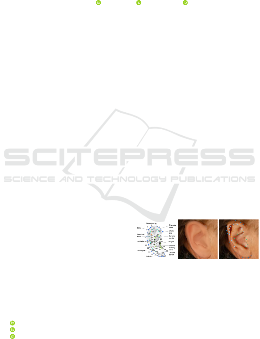
Figure 1: (1) 55 landmarks and their semantics from ITWE-
A dataset (Zhou and Zaferiou, 2017) (2) Rendered densely
corresponded coloured 3D ear mesh projected onto the orig-
inal image (3) Original image marked with predicted land-
marks.
Most modern approaches for 3D face or 3D ear
reconstruction from monocular images fall into three
categories: generation based, regression based and
the combination of both (Tewari et al., 2017). Gen-
eration based methods require a parametric model for
the 3D object and 3D landmarks to optimise a set of
136
Sun, H., Pears, N. and Dai, H.
A Human Ear Reconstruction Autoencoder.
DOI: 10.5220/0010249901360145
In Proceedings of the 16th International Joint Conference on Computer Vision, Imaging and Computer Graphics Theory and Applications (VISIGRAPP 2021) - Volume 5: VISAPP, pages
136-145
ISBN: 978-989-758-488-6
Copyright
c
2021 by SCITEPRESS – Science and Technology Publications, Lda. All rights reserved

parameters for optimal alignment between projected
3D models and 2D landmarks. For 3D ear reconstruc-
tions, two approaches can be found in literature (Dai
et al., 2018; Zhou and Zaferiou, 2017). Regression-
based methods usually utilise neural networks to
regress a parametric model’s parameters directly, as
proposed by (Richardson et al., 2016; Zollh
¨
ofer et al.,
2018) for 3D face reconstruction. Generation-based
methods are often more computationally costly, due
to their non-convex optimisation criteria and the re-
quirement for landmarks. Regression-based methods
require ground truth parameters to be provided, which
is only accessible when using synthetic data (Richard-
son et al., 2016). Otherwise other 3D reconstruction
algorithms are required to obtain ground truth param-
eters beforehand (Zhu et al., 2017). Therefore, Tewari
et al. proposed a self-supervised 3D face reconstruc-
tion method named Model-based Face Autoencoder
(MoFA) that combines both generation and regression
based methods. This aims to mitigate the negative as-
pects of the two categories of method, by using an
autoencoder composed of a regression-based encoder
and a generation-based decoder (Tewari et al., 2017).
However, there are no regression-based or autoen-
coder structured approaches for 3D ear reconstruction
in the literature. Whether this self-supervised autoen-
coder approach can tackle the complexity of the ear
structure remains an open question that we address
here.
The core idea of the self-supervised learning ap-
proach is to synthesise similar colour images from
original colour input images in a differentiable man-
ner. For such an approach, a parametric ear model
is needed. Dai et al. propose a 3D Morphable
Model (3DMM) of the ear, named the York Ear Model
(YEM). Its 3D ear mesh has 7111 vertex coordi-
nates, so 21333 vertex parameters, reduced to 499
shape parameters using PCA. However, to enable
self-supervised learning, the 3D ear meshes require
colour/texture, which is not included in the YEM
model.
In this context, we present a Human Ear Recon-
struction Autoencoder (HERA) system, with the fol-
lowing contributions:
• A 3D ear reconstruction method that is completely
trained unsupervised using in-the-wild monocular
ear colour 2D images.
• An in-the-wild ear colour model that colours the
3D ear mesh to minimise its difference with the
2D ear image in appearance.
• Evaluations that demonstrate that the proposed
model is able to predict a densely corresponded
coloured 3D ear mesh (e.g. Figure 1 (2)) and 2D
landmarks (e.g. Figure 1 (3)).
2 RELATED WORK
In this section, we discuss a range of 3D face recon-
struction methods that utilise an autoencoder structure
to achieve self-supervised learning. The method this
paper proposes obtains 3D ear shapes by employ a
strong prior provided by an ear 3DMM, thus the two
existing 3D parametric ear models will be discussed.
Finally, two methods that evaluate their methods us-
ing normalised landmark error are discussed, since we
evaluate landmark prediction accuracy on the same
dataset, using the same metric.
2.1 Self-supervised Learning for 3D
Dense Face Reconstruction
The self-supervised learning approach to 3D face
reconstruction builds an end-to-end differentiable
pipeline that takes the original colour images as input,
predicts and reconstructs the 3D face mesh, then uses
a differentiable renderer to reconstruct colour images
as output. The goal of such a self-supervised learn-
ing approach is to minimise the difference between
input colour images and output colour images. Sev-
eral novel 3D face reconstruction approaches have re-
cently been proposed. Improvements include using a
face recognition network to contribute to a loss func-
tion, using a Generative Adversarial Network (GAN)
for texture generation (Gecer et al., 2019) and re-
placing the linear 3DMM structure with a non-linear
3DMM (Tran and Liu, 2018). The aim of all of those
approaches is to achieve better performance more in-
tuitively, particularly in terms of minimising the ap-
pearance difference between generated output images
and real input images.
2.2 In-the-wild Ear Image Dataset
There are numerous in-the-wild ear image datasets
built for various purposes, here we focus on Collec-
tion A from the In-the-wild Ear Database (ITWE-A)
since it has 55 manually-marked landmarks. All
the landmarks have semantic meaning, as shown in
Figure 1 (1). This dataset contains 500 images in its
training set and 105 images in its test set, where each
image is captured in-the-wild and contains a clear ear.
The dataset has a large variation in ear colours, as is
the nature of in-the-wild images, and it even contains
several grayscale images. Traditional 3DMM colour
models, such as that of the Basel Face Model 09
(BFM09) (Blanz and Vetter, 1999), often fail to gen-
erate a highly-similar appearance to the input. How-
ever, the in-the-wild ear colour model proposed here,
A Human Ear Reconstruction Autoencoder
137
Input Ear Image
Encoder
(ResNet-18)
Intermediate
Code Vector v
v
v
Ear 3DMM
Ear Colour Model
Shape S
S
S
Colour C
C
C
Differentiable
Renderer
Synthesised Image
Predicted Landmarks
Ground Truth Landmarks
Pixel Loss
Landmark Loss
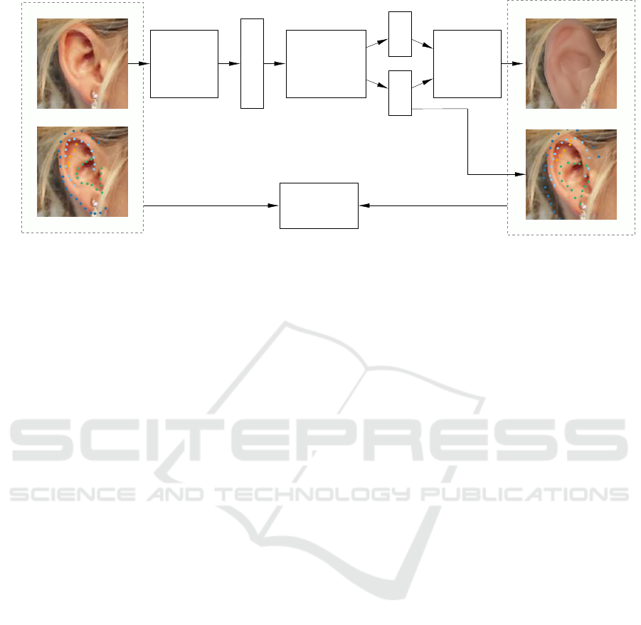
Figure 2: Overview of the autoencoder architecture.
can cover such colour variance, since it models
directly from the in-the-wild images themselves.
2.3 Parametric Ear Models
Zhou and Zaferiou build their parametric ear model
using an Active Appearance Model (AAM), which is
a linear model that aims to model the 2D ear’s shape
and colour simultaneously(Cootes et al., 1998). A
3D Morphable Model (3DMM) is a closely-related
model that models objects’ shapes and colours in 3D
instead of 2D. Blanz and Vetter first proposed a 3D
Morphable Model (3DMM) for human faces (Blanz
and Vetter, 1999), which builds a linear system that
allows different 3D face meshes to be described by
199 shape parameters. Similarly, Dai et al. (Dai
et al., 2018) proposed a 3D morphable model for the
human ear named the York Ear Model (YEM), also
based on a linear system, but with 499 parameters.
Here, we utilise this ear 3DMM for its strong 3D ear
shape prior. Meanwhile, the reduced dimension of
the parameters allows the neural network to perform
a much easier regression task using 499 shape param-
eters rather than 21333 raw vertex parameters.
2.4 2D Ear Detection
Ear detection or localisation in 2D images aims to
find the region of interest bounding the ear, from im-
ages of the human head that contain ears; for exam-
ple, profile-view portraits. It is a vital preprocessing
step in the 3D ear reconstruction pipeline. Object de-
tection has been studied for decades and there exists
a number of algorithms that specifically perform the
2D ear detection task. Zhou and Zaferiou (Zhou and
Zaferiou, 2017) use the histogram of oriented gradi-
ents with a support vector machine (HoG+SVM) to
predict a rectangular region of interest. Emer
ˇ
si
ˇ
c et
al. (Emer
ˇ
si
ˇ
c et al., 2017a) and Bizjak et al. (Bizjak
et al., 2019) propose deep learning methods to tackle
the 2D ear detection task by predicting a pixel-level
segmentation of the 2D ear image directly.
2.5 2D Ear Landmark Localisation
2D ear landmark localisation is a task for finding spe-
cific key points on 2D ear images. It is an intuitive
method of quantitative evaluation of this work where
the shape and alignment of the reconstructed 3D ear
mesh can be evaluated precisely. In 2D face landmark
localisation, numerous approaches obtain 2D land-
marks by reconstructing 3D models first (Zhu et al.,
2017; Liu et al., 2016; McDonagh and Tzimiropou-
los, 2016). Being able to achieve competitive results
against a specialised 2D landmark predictor is neces-
sary for the success of a 3D dense ear reconstruction
algorithm. Zhou and Zaferiou’s approach comes with
the ITWE-A dataset and is considered as a baseline.
They use Scale Invariant Feature Transform (SIFT)
features and an AAM model to predict 2D landmarks
(Zhou and Zaferiou, 2017). Hansley and Segundo
(Hansley et al., 2018) propose a CNN-based approach
to regress 2D landmarks directly and they also evalu-
ate on the ITWE-A dataset. Their approach proposes
two CNNs that both predict the same set of landmarks
but with different strengths. The first CNN has bet-
ter generalisation ability for different ear poses. The
resulting landmarks of the first CNN are used to nor-
malise the ear image. The second CNN predicts im-
proved normalised ear images based on the results of
the first CNN.
VISAPP 2021 - 16th International Conference on Computer Vision Theory and Applications
138

3 THE HERA SYSTEM
Our proposed Human Ear Reconstruction Autoen-
coder (HERA) system employs an autoencoder struc-
ture that takes ear images as input and generates syn-
thetic images. Therefore, it is trained by minimising
the difference between input images and the final syn-
thesised images. An illustration of our end-to-end ar-
chitecture is shown in Figure 2. The encoder is a CNN
predicting intermediate code vectors that are then fed
to the decoder, where coloured 3D ear meshes are re-
constructed and rendered into 2D images.
The decoder is comprised of: (1) the YEM ear
shape model and our in-the-wild ear colour model that
reconstruct ear shapes and ear colours respectively;
(2) PyTorch3D (Ravi et al., 2020) that renders im-
ages with ear shapes and colours in a differentiable
way. The comparison of the input and synthesised
images is implemented by a combination of loss func-
tions and regularisers. The essential loss function is
a photometric loss, with an additional landmark loss
that can be included for both faster convergence time
and better accuracy. The whole autoencoder structure
is designed to be differentiable and so can be trained
in an end-to-end manner. Each part of the architec-
ture (i.e. encoder CNN, ear 3DMM, scaled orthogo-
nal projection and loss functions) is differentiable by
default, thereby using a differentiable renderer to ren-
der 3D meshes to 2D images makes the whole archi-
tecture differentiable. The core part of the decoder is
described in Section 3.1. The whole end-to-end train-
able architecture and the necessary training methods
are then described in Section 3.4.
3.1 Ear 3D Morphable Model
Preliminaries
This section describes the 3DMM part of the decoder
which comprises an ear shape model derived from the
YEM, an ear colour model, and the projection model.
With this 3DMM, the shape parameters α
α
α
s
can be
reconstructed to an 3D ear vertex coordinate vector
S
S
S ∈ R
N×3
where N is the number of vertices in a sin-
gle 3D ear mesh. The colour parameters α
α
α
c
are then
reconstructed to a vertex colour vector C
C
C ∈ R
N×3
to
colour each vertex. The pose parameters p
p
p are used
in the projection model that aligns 3D ear meshes with
2D ears’ pixels.
3.1.1 Ear Shape Model
We employ YEM model (Dai et al., 2018), which
supplies the geometric information necessary for re-
construction. It is constructed using PCA from 500
3D ear meshes and thus provides a strong statistical
prior. The 3D ear vertex coordinate vector (i.e. 3D
ear shape) S
S
S is reconstructed from shape parameter
vector α
α
α
S
by:
S
S
S =
ˆ
S (α
s
) =
¯
S
S
S +U
U
U
s
β
β
β
s
, (1)
where
¯
S
S
S ∈ R
3N
is the mean ear shape, U
U
U
s
∈ R
3N×499
is
the ear shape variation components and the resulting
matrix is rearranged into a N × 3 matrix, where each
row represents a vertex coordinate in 3D space.
The projection model employed is the scaled or-
thogonal projection (SOP) projecting 3D shape to 2D.
Given the 3D ear shape S
S
S from Equation 1, the pro-
jection function,
ˆ
V , is defined as:
V
V
V =
ˆ
V (S
S
S, p
p
p) = f P
P
P
o
ˆ
R(r
r
r) S
S
S + T
T
T , (2)
where P
P
P
o
=
1 0 0
0 1 0
is the orthogonal projection
matrix, V
V
V ∈ R
N×2
are the projected 2D ear vertices
and
ˆ
R(r
r
r) is the function that returns the rotation ma-
trix. Since scaled-orthogonal projection is used, V
V
V
provides sufficient geometric information for the dif-
ferentiable renderer and no additional camera param-
eters are needed.
In addition, 2D landmarks can be extracted from
the projected vertices V
V
V by manually selecting 55 se-
mantically corresponding vertices. Thus we can de-
fine a vector of 2D landmarks of a projected ear shape
V
V
V as:
X
X
X
i
= V
V
V (L
L
L), (3)
where X
X
X
i
∈ R
55×2
are the landmark’s x and y coordi-
nates indexed by L
L
L in the projected ear vertices V
V
V .
3.1.2 In-the-wild Ear Colour Model
The YEM model contains an ear shape model only.
However, the decoder in our architecture requires the
3D ear meshes to be coloured to generate plausible
synthetic ear images. To solve this problem, we build
an in-the-wild ear colour model using PCA whiten-
ing.
Firstly, for each ear image from of the 500 images
from the training set of the ITWE-A dataset, a set of
whitened ear shape model parameters α
α
α
s
and ear pose
p
p
p is fitted using a non-linear optimiser to minimise 2D
landmark distances. Using the reconstruction Equa-
tions 9 ∼ 3, the optimisation criteria E
0
can be formed
as follow:
ˆ
X (α
α
α
s
, p
p
p) =
ˆ
V
ˆ
S (
ˆ
α(α
α
α
s
)), p
p
p
, (4)
E
0
(α
α
α
s
, p
p
p, X
X
X
gt
) =
1
N
L
ˆ
X (α
α
α
s
, p
p
p)
(L
L
L) − X
X
X
gt
2
, (5)
A Human Ear Reconstruction Autoencoder
139

0 -2SD
0 +2SD
1 -3SD
1 +3SD
2 -3SD
2 +3SD
3 -3SD
3 +3SD
4 -3SD
4 +3SD
Mean Colour
Figure 3: In-the-wild Ear Colour Model. The mean colour
and first 5 parameters ± standard deviations (SD) are
shown. The mean 3D ear mesh is used.
where
ˆ
X is the whole reconstruction and projection
function, N
L
= 55 is a constant representing the num-
ber of landmarks and X
X
X
gt
∈ R
55×2
is the ground truth
2D landmarks provided by the ITWE-A dataset.
After the shapes are fitted, the colour for each
vertex is obtained by selecting the corresponding 2D
pixel colour. This process ends up in 500 vertex
colour vectors, which can then be used to build the in-
the-wild ear colour model using PCA whitening. The
vertex colour vectors are parameterised by 40 param-
eters and cover by 86.6% of the colour variation. The
reconstruction coverage rate is not proportional to the
quality of the model building, since setting a moder-
ate coverage rate can implicitly ignore some occlu-
sions (e.g. hair and ear piercings). This colour model
is shown in Figure 3.
The reconstruction of the vertex colour vector C
C
C
is:
C
C
C =
ˆ
C (α
α
α
c
) =
¯
C
C
C +U
U
U
c
α
α
α
c
, (6)
where α
α
α
c
∈ R
40×1
is the colour parameter vector.
¯
C
C
C
is average vertex colour vector, U
U
U
c
is vertex colour
variance component matrix and both are calculated by
the PCA whitening algorithm.
3.2 Intermediate Code Vector
The intermediate code vector
v
v
v =
{
p
p
p, α
α
α
s
, α
α
α
c
}
(7)
connects the encoder and the decoder and has seman-
tic meaning. Where
p
p
p =
{
r
r
r, T
T
T , f
}
(8)
defines the pose of the 3D ear mesh. r
r
r ∈ R
3
is the
azimuth, elevation and row which map to the rotation
matrix through function
ˆ
R(r
r
r) : R
3
→ R
3×3
. T
T
T ∈ R
2×1
defines the translation in X-axis and Y-axis. The
translation in z-axis is not necessary since scaled or-
thogonal projection is used. f is a fraction num-
ber that defines the 3D mesh’s scale. α
α
α
s
∈ R
40×1
are the PCA whitened shape parameters and will be
recovered to the shape parameters β
β
β
s
∈ R
499×1
and
then proceeded by the YEM 3DMM. α
α
α
c
∈ R
40×1
are
the colour parameters for the in-the-wild ear colour
model built by this paper.
3.3 PCA Whitening
To ease the optimisation process in training, we use
PCA whitening to transfer the YEM ear model param-
eters into the format that is more favourable for deep
learning frameworks. Firstly, the variances of the pa-
rameters can differ in a very large scale from 8 × 10
3
for the most significant parameter to 5 × 10
−7
for the
least important parameter. It is difficult to train a neu-
ral network to effectively regress such large variance
data. Secondly, the large number of the parameters
slow the neural networks’ training speed and worse
the optimisation process. This could be mitigated by
trimming a portion of the less important parameters
out. But this has potential to lose the shape and color
information from the trimmed part. To overcome this,
we perform PCA whitening (Kessy et al., 2018) over
the full set of parameters. PCA whitening aims to
generate zero-mean parameters with reduced dimen-
sions in unit-variance. In our experiment, YEM’s
original parameters β
β
β
s
of 499 dimensions are trans-
formed to α
α
α
s
of 40 dimensions while covering 98.1%
of the variance associated with the original parame-
ters. Each original parameter vector β
β
β
s
can be recov-
ered from α
α
α
s
by:
β
β
β
s
=
ˆ
α(α
α
α
s
) = U
U
U
w
α
α
α
s
, (9)
where U
U
U
w
∈ R
499×40
is a constant matrix of variation
components calculated by the PCA whitening pro-
cedure. The original parameters’ mean is not added
since they are zero-mean already.
3.4 Ear Autoencoder
We now combine the intermediate code vector and
decoder components, described in previous sections,
with the encoder, the differentiable renderer and the
loss functions, to build the end-to-end autoencoder
As illustrated in Figure 2, we build an self-
supervised architecture that consists of an encoder,
an intermediate code vector, the decoder components,
the differentiable renderer and the loss for back-
propagation.
The encoder is an 18-layer residual network
(ResNet-18) which is a CNN that performs well on
regression from image data (He et al., 2016). We use
PyTorch3D (Ravi et al., 2020) as a differentiable im-
age renderer developed using PyTorch (Paszke et al.,
2019). It is a differentiable function that maps a set
VISAPP 2021 - 16th International Conference on Computer Vision Theory and Applications
140

of vertex coordinate vector and vertex colour vector
to a 2D image. The encoder Q and decoder W can be
formed as follows:
v
v
v
pred
= Q (I
I
I
in
, θ
θ
θ), (10)
S
S
S
T
pred
,C
C
C
pred
= W
v
v
v
pred
, (11)
I
I
I
pred
= Render
S
S
S
T
pred
,C
C
C
pred
, (12)
X
X
X
pred
= S
S
S
T
pred
(L
L
L), (13)
where I
I
I
in
is the input image and θ
θ
θ are the weights of
the encoder network Q. In the decoder W , the pre-
dicted 3D mesh (i.e. shape with pose S
S
S
T
pred
and colour
C
C
C
pred
) are reconstructed from the predicted interme-
diate code vector v
v
v
pred
. The reconstructed 3D mesh
is then fed to the differential image render for cap-
turing the rendered image I
I
I
pred
. The L
L
L indexes the
x and y coordinates of the 55 ear landmarks in the
ear shape S
S
S. The predicted landmarks X
X
X
pred
∈ R
55×2
can be derived from the predicted ear shape by index-
ing the x and y coordinates of the 55 ear landmarks
in the predicted 3D ear shape from L
L
L. The encoder
ResNet-18 is initialised using the weights pre-trained
on ImageNet (Deng et al., 2009). The trained encoder
network can be used for the shape and color parame-
ters regression.
3.4.1 Loss Function
Our loss function follows the common design of
loss functions in differentiable renderer based self-
supervised 3D reconstruction approaches. The pro-
posed loss function is a combination of four weighted
losses as:
E
loss
= λ
pix
E
pix
(I
I
I
in
) + λ
lm
E
lm
(I
I
I
in
, X
X
X
gt
)
+ λ
reg1
E
reg1
(I
I
I
in
) + λ
reg2
E
reg2
(I
I
I
in
), (14)
where λ
i
are the weights for the losses E
i
.
Pixel Loss. The core idea of the self-supervised ar-
chitecture is that the model can generate synthetic im-
ages from input images and are compared with input
images. Thus to form such comparison, the Mean
Square Error (MSE) is used on all pixels:
E
pix
(I
I
I
in
) = L
MSE
(Render (W (Q (I
I
I
in
, θ
θ
θ))), I
I
I
in
),
(15)
Where L
MSE
is a function that calculates the mean
square error. A pixel mask is used to compare the ren-
dered ear region only, since the rendered ear images
have no background.
Landmark Loss. The optional landmark loss is
used to speed up the training process and help the
network learn 3D ears with better accuracy. Zhou and
Zaferiou (Zhou and Zaferiou, 2017) propose the mean
normalised landmark distance error as their shape
model evaluation metric. Here, we employ it as a part
of the loss function. It can be formed as:
E
lm
(I
I
I
in
, X
X
X
gt
) =
k
(W(Q(I
I
I
in
,θ
θ
θ)))(L
L
L)−X
X
X
gt
k
2
D
N
(
X
X
X
gt
)
N
L
(16)
where X
X
X
gt
is the ground truth landmarks and D
N
(X
X
X
gt
)
is a function gets the diagonal pixel length of the
ground truth landmarks’ bounding box. Since this
loss is optional, setting λ
lm
= 0 can enable the whole
model to be trained on 2D image data I
I
I
in
only, mak-
ing the use of very large-scale unlabelled training data
possible.
Regularisers. Two regularisers are used to con-
strain the learning process and are weighted sepa-
rately. The first regulariser is the statistical plausi-
bility regulariser. The regulariser is formed by:
E
reg1
(I
I
I
in
) =
40
∑
j=1
α
α
α
s j
+
40
∑
j=1
α
α
α
c j
, (17)
where α
α
α
s
and α
α
α
c
are ear shape and colour parameters
predicted by the encoder network. Therefore this pe-
nalises the Mahalanobis distance from the mean shape
and colour.
During our experiments, we found that an addi-
tional restriction on the scale parameter f has to be
applied for the model to be successfully trained with-
out landmarks. The restriction is formed by:
E
reg2
(I
I
I
in
) =
(0.5 − f )
2
if f < 0.5
( f − 1.5)
2
if f > 1.5
0 otherwise
, (18)
We employed two sets of weights, λ, depending on
whether or not landmark loss is used when training.
• Training with landmarks: λ
pix
= 10, λ
lm
= 1,
λ
reg1
= 5 × 10
−
2 and λ
reg2
= 0
• Training without landmarks: λ
pix
= 2, λ
lm
= 0,
λ
reg1
= 5 × 10
−
2 and λ
reg2
= 100
3.4.2 Dataset Augmentation
Since the ITWE-A dataset used to train our model
contains only 500 landmarked ear images, having lim-
ited variance on ear rotations, we perform data aug-
mentation on the original dataset. An ear direction of
a 2D ear image is defined by a 2D vector from one
of the ear lobe landmark points to one of the ear he-
lix landmark points. For each 2D ear image, 12 ran-
dom rotations around its central point are applied such
that the angles between their ear directions and the Y-
axis of the original image are uniformly distributed
A Human Ear Reconstruction Autoencoder
141
between −60
◦
and 60
◦
. The augmented ear image
dataset contains 6, 000 images in total. With this aug-
mentation, we find that test set landmark error drops
significantly.
4 RESULTS
In this section, both quantitative evaluation results and
qualitative evaluation results are discussed. Quanti-
tative evaluation focuses on comparing landmark fit-
ting accuracy with different approaches. While the
qualitative evaluation focuses on evaluating the vi-
sual results of this 3D ear reconstruction algorithm.
Furthermore, an ablation study is conducted to anal-
yse the improvement that various optimisations of this
work has proposed, including the PCA whitening on
the YEM model parameters, the statistical plausibil-
ity regulariser and the dataset augmentation. The ab-
breviation Human Ear Reconstruction Autoencoder
(HERA) is used to represent the final version of this
work.
4.1 Quantitative Evaluations
Table 1: Normalised landmark distance error statistics on
ITWE-A.
Method mean ± std median ≤ 0.1 ≤ 0.06
Zhou & Zaferiou 0.0522 ± 0.024 0.0453 95% 78%
HERA 0
0
0.
.
.0
0
03
3
39
9
98
8
8 ±
±
± 0
0
0.
.
.0
0
00
0
09
9
9 0
0
0.
.
.0
0
03
3
39
9
91
1
1 1
1
10
0
00
0
0% 9
9
96
6
6.
.
.2
2
2%
HERA-W/O-AUG-LM 0.0591 ± 0.014 0.0567 99% 64.7%
The main quantitative evaluation method applied is
the mean normalised landmark distance error pro-
posed by (Zhou and Zaferiou, 2017) formed in Equa-
tion 16 which also forms the landmark loss that trains
our system. Projecting the 3D ear meshes’ key points
to 2D and comparing them with the ground truth can
assess the accuracy of the 3D reconstruction. There
are two approaches that predict the same set of land-
marks using the same dataset in the literature , there-
fore comparisons can be formed. Zhou & Zaferiou’s
work (Zhou and Zaferiou, 2017) is considered as
a baseline solution and Hansley & Segundo’s work
(Hansley et al., 2018) is a specifically designed 2D
landmark localisation algorithm that has the lowest
landmark error in the literature. To interpret the land-
mark error, it is stated that for an acceptable predic-
tion of landmarks, the mean normalised landmark dis-
tance error has to be below 0.1 (Zhou and Zaferiou,
2017). This is a dimensionless metric that is the ra-
tio of the mean Euclidean pixel error to the diagonal
length of the ear bounding box.
As this paper stated in Section 3.4.1, HERA can
be trained without landmarks or data augmentation
in a self-supervised manner. The HERA version that
0 0.01 0.02 0.03 0.04
0.05 0.06
0.07 0.08 0.09 0.1
0
0.1
0.2
0.3
0.4
0.5
0.6
0.7
0.8
0.9
1
Landmark error
Percentage of images
HERA
Hansley & Segundo
Zhou & Zaferiou
HERA-W/O-AUG-LM
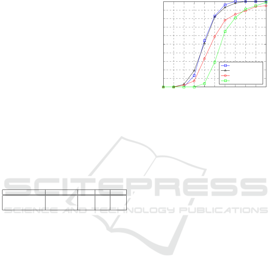
Figure 4: Cumulative error distribution curve compari-
son among different landmark detection algorithms and our
work.
uses no landmark loss during training and trains on
the original 500 ear images is named HERA-W/O-
AUG-LM.
Our HERA system is now compared with Zhou
& Zaferiou’s and Hansley & Segundo’s work regard-
ing the normalised landmark error’s mean, standard
deviation, median and cumulative error distribution
(CED) curve evaluated on the test set of ITWE-A
which contains 105 ear images. The numerical results
are shown in Table 1 and the CED curve is shown in 4.
Additionally, the percentage of predictions that have
error less than 0.1 and 0.6 are given in Table 1.
From Table 1 and Figure 4, it can be concluded
that HERA outperforms Zhou & Zaferiou’s work by
a large margin in terms of 2D landmark localisation
task. When compared with Hansley & Segundo’s 2D
landmark localisation work, similar results are shown.
This is considered acceptable when comparing a 3D
reconstruction algorithm with a 2D landmark local-
isation algorithm. Hansley & Segundo’s landmark
localiser is comprised of two specifically designed
CNNs for landmark regressions while HERA uses
only one CNN to regress a richer set of information
(i.e. pose, 3D model’s parameters and colour param-
eters). Regarding the threshold of 0.1 proposed by
(Zhou and Zaferiou, 2017), both HERA and Hansley
& Segundo’s work are 100% below 0.1, and HERA
trained without landmarks achieves 99% below 0.1.
The CED curves show that, although HERA-W/O-
AUG-LM performs worse than Zhou & Zaferiou’s
work in the error region below around 0.077, our per-
formance is better at the 0.1 error point. In other
words, HERA-W/O-AUG-LM can predict landmarks
with less than 0.1 error more consistently than the
baseline.
VISAPP 2021 - 16th International Conference on Computer Vision Theory and Applications
142
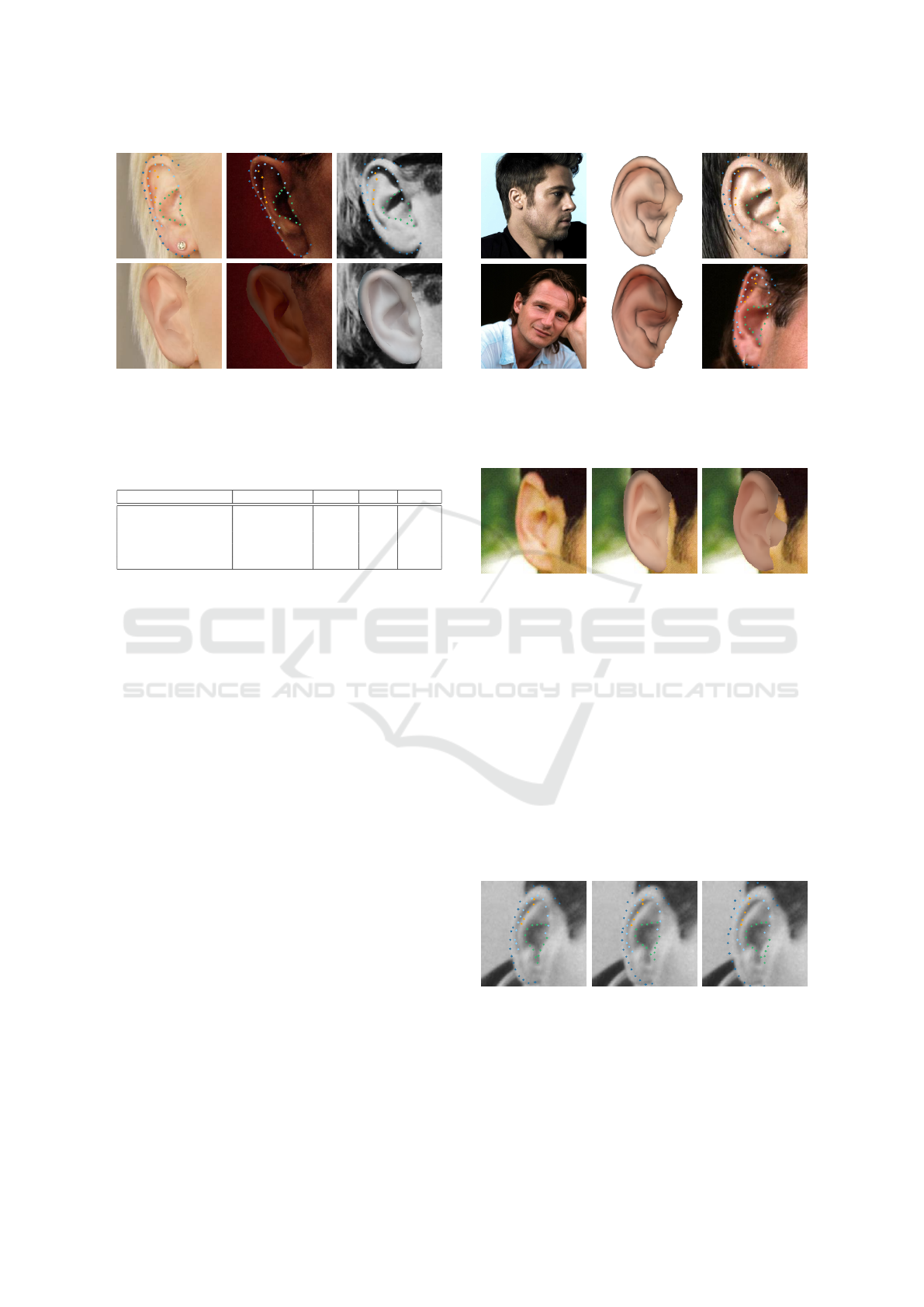
Figure 5: Test set prediction results with different ear
colours. Top row: original ear images marked with pre-
dicted 2D landmarks. Bottom row: predicted 3D ear meshes
projected onto original ear images.
Table 2: Normalised landmark distance error statistics on
ITWE-A for ablation study.
Method mean ± std median ≤ 0.1 ≤ 0.06
HERA 0.0398 ± 0.009 0.0391 100% 96.2%
HERA-W/O-WTN 0.0401 ± 0.009 0.0384 100% 96.2%
HERA-W/O-PIX 0.0392 ± 0.009 0.0387 100% 96.2%
HERA-W/O-AUG 0.0446 ± 0.011 0.0437 100% 92.4%
HERA-W/O-AUG-LM 0.0591 ± 0.014 0.0567 99% 64.7%
4.2 Qualitative Evaluations
Qualitative evaluations of this work focus on visually
showing the 3D reconstruction results on ITWE-A’s
test set. In Figure 5, three images with large colour
variation are predicted, the top row shows the 2D
landmark predictions look reasonable. The compar-
ison between the top row and the bottom row shows
that the quality of the reconstructed 3D meshes are
reasonable in geometric aspect, while the in-the-wild
colour model can reconstruct a large variation of in-
the-wild ear colours even from grayscale images.
In Figure 6, two images with different head poses
are selected for 3D ear reconstruction. The top row
shows the results from a near-ideal head pose (i.e.
near-profile face) and the bottom row shows the re-
sults from a large head pose deviation from the ideal
(i.e. front facing, tilted head). The figure shows that
HERA works well with different head poses. For the
front facing images, the model predicts the correct
horizontal rotation rather than narrowing the 3D ear
mesh’s width to match the 2D image.
4.3 Ablation Study
We now study how each component can affect
HERA’s performance and we evaluate on several sys-
tem variations including HERA-W/O-WTN (with-
out PCA whitening on 3D ear shape parameters β
β
β
s
),
HERA-W/O-PIX (without pixel loss), HERA-W/O-
Figure 6: Test set prediction results with different head
poses. Each row represents a distinct subject. 1
st
column:
Original uncropped images. 2
nd
column: Predicted 3D ear
meshes. 3
rd
column: Predicted 2D landmarks. Ear pose is
successfully predicted when difficult head pose involves.
(2)(1) (3)
Figure 7: Appearance comparison between the recon-
structed 3D ear meshes of (1) Ground truth input image, (2)
HERA and (3) HERA-W/O-PIX (without using the pixel
error). Although the landmark errors are similar, not using
pixel error results in a rendered image with more appear-
ance difference.
AUG (without data augmentation) and HERA-W/O-
AUG-LM (without landmark loss).
Table 2 shows the statistics for all the variations of
HERA. When training without PCA whitening on 3D
ear shape parameters and without pixel loss, perfor-
mance on 2D landmark localisation is similar to the
final proposed method. However, using PCA whiten-
ing balances the parameters for the neural network to
predict and therefore acts as a better underlying de-
(1) (2) (3)
Figure 8: 2D landmark localisation comparison between
the prediction results of (1) HERA, (2) HERA-W/O-AUG
(without data augmentation) and (3) HERA-W/O-AUG-LM
(without data augmentation or landmark error). Data aug-
mentation enables better ear rotation prediction and land-
mark loss is vital to accurate alignment especially for the
ear contour part.
A Human Ear Reconstruction Autoencoder
143

sign choice. The major contribution of applying PCA
whitening in this work is that it speeds up the training
process by more than 30% per epoch on a GPU. In
the meantime, a balanced design of intermediate code
vector with similar variance for each parameter can
benefit the performance of the neural network. The
proposed HERA system then takes ∼ 70 seconds to
train one epoch on an NVIDIA RTX 2080 and takes
∼ 350 epochs to train the whole network. After train-
ing, the network predicts a single image in 6 ms.
For training without pixel loss, as shown in Figure
7, the overall appearance of the rendered ear image
differs from the input ear image especially for the he-
lix part. Training without pixel loss makes the model
focus on lowering the landmark alignment error re-
gardless of the overall appearance of the ear. There-
fore it is necessary to utilise the pixel loss. This set of
figures also illustrates the pose ambiguity of this sys-
tem caused by orthogonal projection. For a distinct
set of ear 3DMM parameters, there exists two differ-
ent rotations that result in the same projected 2D land-
marks. In one case, such as Figure 7 (1), the external
auditory canal part of the ear is visible and in the other
case such as the other rendered images in this paper,
the external auditory canal is covered by itself. This
ambiguity may affect further applications that relate
the reconstructed 3D ear and other 3D objects, such
as the 3D head, but a simple 3D registration task can
be carried out to solve the rotational ambiguity, if re-
quired. Restrictions on the rotations during the train-
ing phase can be applied to allow the results to fall
into desired range.
When training without data augmentation, the 2D
landmark localisation performance drops by a small
amount mainly due to its lack of variety in ear rota-
tion, shown in Figure 8. When training without land-
mark loss, the predicted landmarks is not accurate
enough, shown in Figure 8. As a result, the recon-
structed 3D ears are not accurately aligned with the
2D ears especially for the ear contours.
5 CONCLUSION
As a large proportion of human-related 3D recon-
struction approaches focus on the human face, 3D ear
reconstruction, as an important human-related task,
has much less related work. In this paper, we propose
a self-supervised deep 3D ear reconstruction autoen-
coder from single image. Our model reconstructs the
3D ear mesh with a plausible appearance and accurate
dense alignment, as witnessed by the accurate align-
ment compared to ground truth landmarks. The com-
prehensive evaluation shows that our method achieves
state-of-the-art performance in 3D ear reconstruction
and 3D ear alignment.
REFERENCES
Bizjak, M., Peer, P., and Emer
ˇ
si
ˇ
c,
ˇ
Z. (2019). Mask r-cnn for
ear detection. In 2019 42nd International Convention
on Information and Communication Technology, Elec-
tronics and Microelectronics (MIPRO), pages 1624–
1628. IEEE.
Blanz, V. and Vetter, T. (1999). A morphable model for
the synthesis of 3d faces. In Proceedings of the 26th
annual conference on Computer graphics and inter-
active techniques, pages 187–194.
Cootes, T. F., Edwards, G. J., and Taylor, C. J. (1998). Ac-
tive appearance models. In European conference on
computer vision, pages 484–498. Springer.
Dai, H., Pears, N., Huber, P., and Smith, W. A. (2020a).
3d morphable models: The face, ear and head. In 3D
Imaging, Analysis and Applications, pages 463–512.
Springer.
Dai, H., Pears, N., and Smith, W. (2018). A data-augmented
3d morphable model of the ear. In 2018 13th IEEE In-
ternational Conference on Automatic Face & Gesture
Recognition (FG 2018), pages 404–408. IEEE.
Dai, H., Pears, N., and Smith, W. (2019). Augmenting a 3d
morphable model of the human head with high resolu-
tion ears. Pattern Recognition Letters, 128:378–384.
Dai, H., Pears, N., Smith, W., and Duncan, C. (2020b). Sta-
tistical modeling of craniofacial shape and texture. In-
ternational Journal of Computer Vision, 128(2):547–
571.
Deng, J., Dong, W., Socher, R., Li, L.-J., Li, K., and Fei-
Fei, L. (2009). Imagenet: A large-scale hierarchical
image database. In 2009 IEEE conference on com-
puter vision and pattern recognition, pages 248–255.
Ieee.
Emer
ˇ
si
ˇ
c,
ˇ
Z., Gabriel, L. L.,
ˇ
Struc, V., and Peer, P. (2017a).
Pixel-wise ear detection with convolutional encoder-
decoder networks. arXiv preprint arXiv:1702.00307.
Emer
ˇ
si
ˇ
c,
ˇ
Z.,
ˇ
Struc, V., and Peer, P. (2017b). Ear recognition:
More than a survey. Neurocomputing, 255:26–39.
Emer
ˇ
si
ˇ
c,
ˇ
Z., SV, A. K., Harish, B., Gutfeter, W., Khiarak,
J., Pacut, A., Hansley, E., Segundo, M. P., Sarkar, S.,
Park, H., et al. (2019). The unconstrained ear recog-
nition challenge 2019. In 2019 International Confer-
ence on Biometrics (ICB), pages 1–15. IEEE.
Gecer, B., Ploumpis, S., Kotsia, I., and Zafeiriou, S. (2019).
Ganfit: Generative adversarial network fitting for high
fidelity 3d face reconstruction. In Proceedings of the
IEEE Conference on Computer Vision and Pattern
Recognition, pages 1155–1164.
Hansley, E. E., Segundo, M. P., and Sarkar, S. (2018). Em-
ploying fusion of learned and handcrafted features
for unconstrained ear recognition. IET Biometrics,
7(3):215–223.
He, K., Zhang, X., Ren, S., and Sun, J. (2016). Deep resid-
ual learning for image recognition. In Proceedings of
VISAPP 2021 - 16th International Conference on Computer Vision Theory and Applications
144

the IEEE conference on computer vision and pattern
recognition, pages 770–778.
Kessy, A., Lewin, A., and Strimmer, K. (2018). Optimal
whitening and decorrelation. The American Statisti-
cian, 72(4):309–314.
Liu, F., Zeng, D., Zhao, Q., and Liu, X. (2016). Joint
face alignment and 3d face reconstruction. In Euro-
pean Conference on Computer Vision, pages 545–560.
Springer.
McDonagh, J. and Tzimiropoulos, G. (2016). Joint face de-
tection and alignment with a deformable hough trans-
form model. In European Conference on Computer
Vision, pages 569–580. Springer.
Paszke, A., Gross, S., Massa, F., Lerer, A., Bradbury, J.,
Chanan, G., Killeen, T., Lin, Z., Gimelshein, N.,
Antiga, L., et al. (2019). Pytorch: An imperative
style, high-performance deep learning library. In
Advances in neural information processing systems,
pages 8026–8037.
Ploumpis, S., Ververas, E., O’Sullivan, E., Moschoglou,
S., Wang, H., Pears, N., Smith, W., Gecer, B., and
Zafeiriou, S. P. (2020). Towards a complete 3d mor-
phable model of the human head. IEEE Transactions
on Pattern Analysis and Machine Intelligence.
Ravi, N., Reizenstein, J., Novotny, D., Gordon, T., Lo, W.-
Y., Johnson, J., and Gkioxari, G. (2020). Accelerating
3d deep learning with pytorch3d. arXiv:2007.08501.
Richardson, E., Sela, M., and Kimmel, R. (2016). 3d
face reconstruction by learning from synthetic data.
In 2016 fourth international conference on 3D vision
(3DV), pages 460–469. IEEE.
Tewari, A., Zollhofer, M., Kim, H., Garrido, P., Bernard,
F., Perez, P., and Theobalt, C. (2017). Mofa: Model-
based deep convolutional face autoencoder for unsu-
pervised monocular reconstruction. In Proceedings of
the IEEE International Conference on Computer Vi-
sion Workshops, pages 1274–1283.
Tran, L. and Liu, X. (2018). Nonlinear 3d face morphable
model. In Proceedings of the IEEE conference on
computer vision and pattern recognition, pages 7346–
7355.
Zhou, Y. and Zaferiou, S. (2017). Deformable models of
ears in-the-wild for alignment and recognition. In
2017 12th IEEE International Conference on Auto-
matic Face & Gesture Recognition (FG 2017), pages
626–633. IEEE.
Zhu, X., Liu, X., Lei, Z., and Li, S. Z. (2017). Face align-
ment in full pose range: A 3d total solution. IEEE
transactions on pattern analysis and machine intelli-
gence, 41(1):78–92.
Zollh
¨
ofer, M., Thies, J., Garrido, P., Bradley, D., Beeler, T.,
P
´
erez, P., Stamminger, M., Nießner, M., and Theobalt,
C. (2018). State of the art on monocular 3d face re-
construction, tracking, and applications. In Computer
Graphics Forum, volume 37, pages 523–550. Wiley
Online Library.
A Human Ear Reconstruction Autoencoder
145
