
Estimation of Movement Speed in Monitoring
Systems based on Sensors of Multiple Types
Jakub Wagner
a
and Paweł Mazurek
b
Institute of Radioelectronics and Multimedia Technology, Warsaw University of Technology, Warsaw, Poland
Keywords: Healthcare, Monitoring, Data Fusion, Numerical Differentiation, Regularisation, Total Variation.
Abstract: The research reported in this paper is related to the differentiation and fusion of measurement data in systems
for healthcare-oriented unobtrusive monitoring of elderly persons. Two methods for regularised numerical
differentiation – suitable for different shapes of trajectories of the monitored person’s movement – are con-
sidered. A technique for the fusion of data from sensors of different types – which involves weighting those
data according to the available a priori information about the variances of errors corrupting those data – is
presented. Guidelines on the usage and optimisation of that technique are provided according to the results of
numerical experimentation based on synthetic data.
1 INTRODUCTION
1.1 Motivation for Monitoring
The life expectancy at birth, estimated for the global
population in 2019, is ca. 73 years; it has been rising
during the last decades and is predicted to reach 77
years by the half of the twenty-first century, while the
global fertility rate – i.e. the number of live births per
woman over a lifetime – is decreasing (United
Nations, 2019). For these reasons, the global popula-
tion is ageing, i.e. the share of people aged at least 65
years is growing. Taking into account these predic-
tions, several global institutions involved in the pro-
tection and management of public health have point-
ed out the necessity to take actions aimed at improv-
ing the quality of life of elderly people and at ensuring
that the public expenditures, related to the healthcare
services addressed to those people, remain affordable
(see, for example, WHO, 2017). That necessity has
inspired the development of diverse technological
means, designed to facilitate the accomplishment of
various healthcare-related objectives such as the re-
duction of the number of admissions to nursing
homes, the optimisation of the processes of treatment
or rehabilitation, or the social integration of elderly
people. For instance:
a
https://orcid.org/0000-0002-2739-4578
b
https://orcid.org/0000-0002-8239-4589
Alerting devices – such as those worn on the body
or clothes, which send out an emergency signal
when a button is pressed – reduce the delay of in-
tervention after dangerous events such as falls,
and enhance the sense of safety of elderly people
who live independently in their households, thus
encouraging them to stay active (Fleming and
Brayne, 2008).
Robots support elderly people in tasks which they
are unable to complete without aid, and may
relieve them from the sense of loneliness (Wada
et al., 2004, Sharkey and Sharkey, 2012).
Sensors and actuators ensuring the safe function-
ing of household appliances protect elderly people
from dangerous accidents (Al-Shaqi et al., 2016).
Video games which involve players in physical
activity may be used to promote such activity
among elderly people and gather information
about their health status (Garcia Marin, 2015).
Social-networking websites and systems based on
ambient-display screens – designed to help elder-
ly people maintain contact with their relatives and
friends – help prevent their social isolation
(Campos et al., 2016).
Monitoring systems provide data representative of
the behaviour and physiological parameters of in-
dependently-living elderly people, help in identi-
fying progressive changes in those people’s health
Wagner, J. and Mazurek, P.
Estimation of Movement Speed in Monitoring Systems based on Sensors of Multiple Types.
DOI: 10.5220/0010249300690079
In Proceedings of the 14th International Joint Conference on Biomedical Engineering Systems and Technologies (BIOSTEC 2021) - Volume 4: BIOSIGNALS, pages 69-79
ISBN: 978-989-758-490-9
Copyright
c
2021 by SCITEPRESS – Science and Technology Publications, Lda. All rights reserved
69

status and enable quick reactions to dangerous ac-
cidents (Peetoom et al., 2015).
This study is focused on technological solutions
belonging to the last category, viz. on monitoring
systems which enable the acquisition of data repre-
sentative of the monitored person’s movement tra-
jectory. Such data can be used to obtain information
useful for the healthcare practitioners, in particular –
to estimate the monitored person’s walking speed.
Walking is a complex task which requires the interac-
tion of several organs and the proper functioning of
multiple parts of the brain (Kikkert et al., 2016). The
analysis of gait can provide information about the so-
called functional mobility, i.e. a set of abilities related
to balance and gait manoeuvres used in everyday life
– abilities which partially reflect the overall health
status (Shumway-Cook et al., 2000). Some quantities
characterising the gait – such as the stride length, the
stride frequency, or the variability of the stride time –
are correlated with the risk of falling and are useful as
indicators of conditions such as Parkinson’s disease,
osteoarthritis or diabetes (Hodgins, 2008). On the
other hand, the speed with which a person walks com-
fortably during every-day activities – the so-called
self-selected walking speed – has been recently recog-
nised as a versatile, informative and easily measur-
able indicator of functional mobility and general
health status (Lusardi, 2012):
its values smaller than 0.6 m/s indicate a high risk
of fall and hospitalisation;
its increase of at least 0.1 m/s is a useful predictor
of well-being;
its similar decrease is correlated with the deterio-
ration of the health status or the decline in overall
functioning.
In clinical settings, self-selected walking speed
can be estimated by using a stopwatch to measure the
time which the examined person needs to walk along
a path of a predefined length; however, the in-home
use of monitoring systems may prove to be more re-
liable, convenient and affordable than clinical assess-
ment sessions (Hagler et al., 2010).
Apart from the estimation of the self-selected
walking speed, the data representative of the monitor-
ed person’s two- or three-dimensional movement tra-
jectory – together with the estimates of velocity and
acceleration, obtained on the basis of those data – can
be used in other healthcare-oriented applications,
such as the detection of falls (Khan and Hoey, 2017)
or the analysis of that person’s behavioural patterns
(Baldewijns et al., 2016), which may enable the early
detection of the onset of dementia.
1.2 Techniques for Monitoring
In the practice of healthcare-oriented monitoring, the
solutions based on wearable sensors – i.e. sensors
attached to the body or clothes of the monitored per-
son, including accelerometers, gyroscopes and sen-
sors of physiological parameters – are the most wide-
spread ones (Majumder et al., 2017). The most im-
portant drawback of such techniques is the fact that
the need to wear devices may be considered inconve-
nient by the people subject to monitoring; further-
more, a system based on wearable devices becomes
useless if the monitored person forgets to wear the
device or decides not to do it. For these reasons, it
seems desirable to develop monitoring systems which
do not require any action from the monitored persons.
Other monitoring techniques, already applied in
healthcare practice, include those based on video
cameras, passive-infrared detectors of motion and
pressure sensors. There are also two emerging cate-
gories of monitoring techniques which attract grow-
ing attention of researchers, viz. techniques based on
depth sensors and impulse-radar sensors. The recent
attempts to apply them for monitoring of elderly per-
sons are mainly motivated by the conviction that they
may be less intrusive, invasive and cumbersome than
the above-mentioned, better explored techniques.
This study is devoted to the monitoring techniques
which – like those based on depth sensors and im-
pulse-radar sensors – involve the estimation of the
position of the monitored person’s centre of mass
with high temporal resolution (i.e. several to several
dozen estimates per second), followed by the analysis
of the sequences of those estimates. Such techniques
require numerical differentiation in order to estimate
the monitored person’s movement speed. The posi-
tion estimates are corrupted with measurement errors,
so their numerical differentiation is an ill-posed prob-
lem, i.e. if no remedies are applied, small errors cor-
rupting the data may cause large errors in the speed
estimates. Therefore, the problem of numerical differ-
entiation needs to be regularised, i.e. redefined in
such a way as to ensure a kind of “regularity” of the
speed estimates, at the cost of limiting their attainable
fidelity to the measurement data, in order to reduce
their sensitivity to the measurement errors.
Sensors which operate according to different phy-
sical principles tend to have specific complementary
advantages and disadvantages; for example, impulse-
radar sensors offer a broad field of view and the ca-
pacity of through-the-wall monitoring, but provide
estimates of the monitored person’s position corrupt-
ed with larger errors than depth sensors, which – on
the other hand – cannot detect occluded persons and
BIOSIGNALS 2021 - 14th International Conference on Bio-inspired Systems and Signal Processing
70

whose field of view is limited. This study is devoted
to monitoring systems which employ sensors of mul-
tiple types and thus require the application of an ade-
quate method for the fusion of data acquired by means
of those sensors.
Despite the generally recognised need for devel-
oping technological solutions aimed at improving the
quality of life of elderly people and contributing to
the efficiency of public health management, health-
care-oriented monitoring systems are still not being
commonly used in healthcare facilities and house-
holds. This may be explained by the difficulties relat-
ed to the development of technological solutions
which can be both widely accepted among elderly
people and – at the same time – capable of providing
healthcare practitioners with useful information
(Debes et al., 2016). Solutions aimed at combining
the complementary advantages of several types of
sensors seem to have a promising potential for
achieving a satisfactory compromise between the two
above-mentioned qualitites.
1.3 Scope of Study
Two methods of numerical differentiation have been
considered in this study (cf. Subsection 2.2):
a method based on Tikhonov regularisation, suit-
able for the analysis of smooth movement trajec-
tories;
a method based on total-variation regularisation,
suitable for the analysis of piecewise-linear move-
ment trajectories.
In both cases, the fusion of data from different sensors
has been performed by adopting an adequate indicator
of the fidelity of the speed estimates to the measure-
ment data (cf. Subsection 2.3). The aim of this study
is the analysis of the properties and applicability of
that indicator – the analysis based on the results of
experiments performed using synthetic data.
2 ESTIMATION OF MOVEMENT
SPEED
2.1 Mathematical Formulation of
Research Problem
Let’s assume that the time-dependence of the mon-
itored person’s position in a given direction can be
modelled using a scalar, real-valued function
𝑓: ℝ → ℝ of a scalar variable
t
modelling time,
differentiable on the interval
0,T
. The analytic
form of
f
is unknown. The available data
1
,,
N
x
x
are its error-corrupted values, resulting from mea-
surements performed at time instants
1
,,
N
tt
such
that
1
0
N
ttT
. Those data are modelled as
follows:
nnn
xft
for
1, ,nN
(1)
where
1
,,
N
are realisations of independent ran-
dom variables
1
,,
N
modelling measurement er-
rors. Since it is assumed that those data may have
been acquired by means of different types of sensors,
the distributions of the variables
1
,,
N
may dif-
fer; in this study, it is assumed that those variables are
zero-mean, normally distributed and that their vari-
ances are
22
1
,,
N
. Those variances are unknown,
but their estimates
22
1
ˆˆ
,,
N
are available; in prac-
tice, these estimates may be obtained as a result of
prior calibration experiments.
The time-dependence of the monitored person’s
speed in the given direction is modelled with
1
f
, i.e.
the first derivative of
f
. Speed estimates
1
1
ˆ
,,x
1
ˆ
N
x
are sought such that:
11
ˆ
nn
x
ft
for
1, ,nN
(2)
2.2 Numerical Differentiation
The procedure for numerical differentiation, i.e. de-
termination of the sequence
11
1
ˆˆ
,,
N
x
x
on the basis
of the sequence
1
,,
N
x
x
, involves the following
operations:
approximation of the function
f
,
computation of the first derivative
1
ˆ
f
of the re-
sult of approximation
ˆ
f
,
evaluation of
1
ˆ
f
at the time instants
1
,,
N
tt
.
The approximation of
f
requires the determination
of a set of admissible approximating functions and the
selection of one of them on the basis of the data
n
x
.
In this study, it is assumed that the admissible approx-
imating functions are polynomial splines of degree 2.
Such functions are defined as quadratic polynomials
in each subinterval
1
,
nn
tt
,
1, , 1nN
; hence,
it can be easily checked that the following equality is
satisfied for each such function
ˆ
f
:
Estimation of Movement Speed in Monitoring Systems based on Sensors of Multiple Types
71

(3)
fo
r
Thus:
(4)
for
The
1N
equations obtained by evaluating Eq. (4)
for
2, ,nN
– the equations specifying the linear
relation between the values of the approximating
function and the values of its first derivative – may be
supplemented by adopting an additional assumption
regarding the movement of the monitoring person;
here, it has been assumed that the speed of the moni-
tored person is constant at the beginning of the time
interval under analysis, i.e.:
11
12
ˆˆ
0ft ft
(5)
Eq. (4) and Eq. (5) may be collected in the following
way:
1
ˆˆ
Qx x
(6)
where
ˆ
x
is the vector of values of the approximating
function, shifted by
1
ˆ
f
t
:
T
1121 1
ˆˆˆˆ ˆ ˆ
ˆ
N
ft ft ft ft ft ft
x
1
ˆ
x
is the vector of estimates of the first derivative:
T
T
111 1 1
11
ˆˆ
ˆˆˆ
NN
x x ft ft
x
and the matrix
Q
is defined as follows:
21 21
31 32
21
31 1
21 4 2
22
222
222 2
110
0
0
NN
tt tt
NN
tt tt
tt
tt t t
tt tt
Q
R
If the measurement errors are negligible and – conse-
quently – one may assume that the best approximat-
ing function is the one which interpolates the mea-
surement data,
i.e.
ˆ
nn
f
tx
for
1, ,nN
, then
Eq. (6) can be used directly to obtain the vector
1
ˆ
x
of speed estimates,
viz.:
1
1
ˆ
xQx
(7)
where
x
is the vector of measurement data shifted
by
1
x
:
T
112 1 1N
x
xx x x x
x
However, the condition number of
Q
tends to be
very large even for relatively small
N, and thus the
speed estimates obtained this way are unacceptably
inaccurate even when the errors corrupting the data
are small. The remedy for this is regularisation, which
consists in imposing an additional constraint on the
set of admissible approximating functions. Such a
constraint should be based on a realistic
a priori as-
sumption regarding the movement of the monitored
person, in particular – an assumption about the shape
of the function
f
modelling the trajectory of that
movement. In this study, constraints on the following
two quantities are considered:
the squared 2-norm of the vector of values of the
second derivative of the approximating function,
denoted with
hereinafter:
(8)
where and:
the squared 1-norm of the vector of values of the
second derivative of the approximating function,
denoted with
hereinafter:
2
22
22 1
11
1
ˆ
ˆˆ
N
n
n
ft
xDx
(9)
The imposition of a constraint on
– being a va-
riant of the regularisation technique commonly re-
ferred to as Tikhonov regularisation (Stickel, 2010) –
is suitable when the monitored person’s movement
trajectory is adequately modelled with a smooth func-
tion, i.e. a function whose several derivatives are con-
tinuous. Such an assumption about the shape of the
modelling function seems reasonable when human
movement is analysed in a relatively short time inter-
val; for example, during gait, the position of the mon-
itored person’s centre of mass along the direction or-
thogonal to the walking direction fluctuates smoothly
with a period corresponding to the stride duration.
11
1
11
ˆˆ ˆ ˆ
2
nn
nn n n
tt
ft ft f t f t
2, ,nN
111
1
11
1
22
2
ˆˆˆ ˆ
nn
n
tt t t
nn
ft ft f t f t
21
1
1
2
ˆ
tt
ft
2, ,nN
2
22
22 1
22
1
ˆ
ˆˆ
N
n
n
ft
xDx
T
22 2
1
ˆˆ
ˆ
N
ft ft
x
21 21
32 32
11
11
11
1
11
0
00
0
NN NN
tt tt
tt tt
NN
tt tt
D
R
BIOSIGNALS 2021 - 14th International Conference on Bio-inspired Systems and Signal Processing
72
On the other hand, the imposition of a constraint
on
– being a variant of the regularisation technique
commonly referred to as total-variation (TV) regu-
larisation (Rudin et al., 1992) – is suitable when the
movement trajectory is adequately modelled with a
piecewise-linear function. Such an assumption seems
reasonable when the walking trajectory is modelled in
a time interval of several seconds or minutes, since
people tend to walk with approximately piecewise-
constant speed.
The effects of both considered regularisation tech-
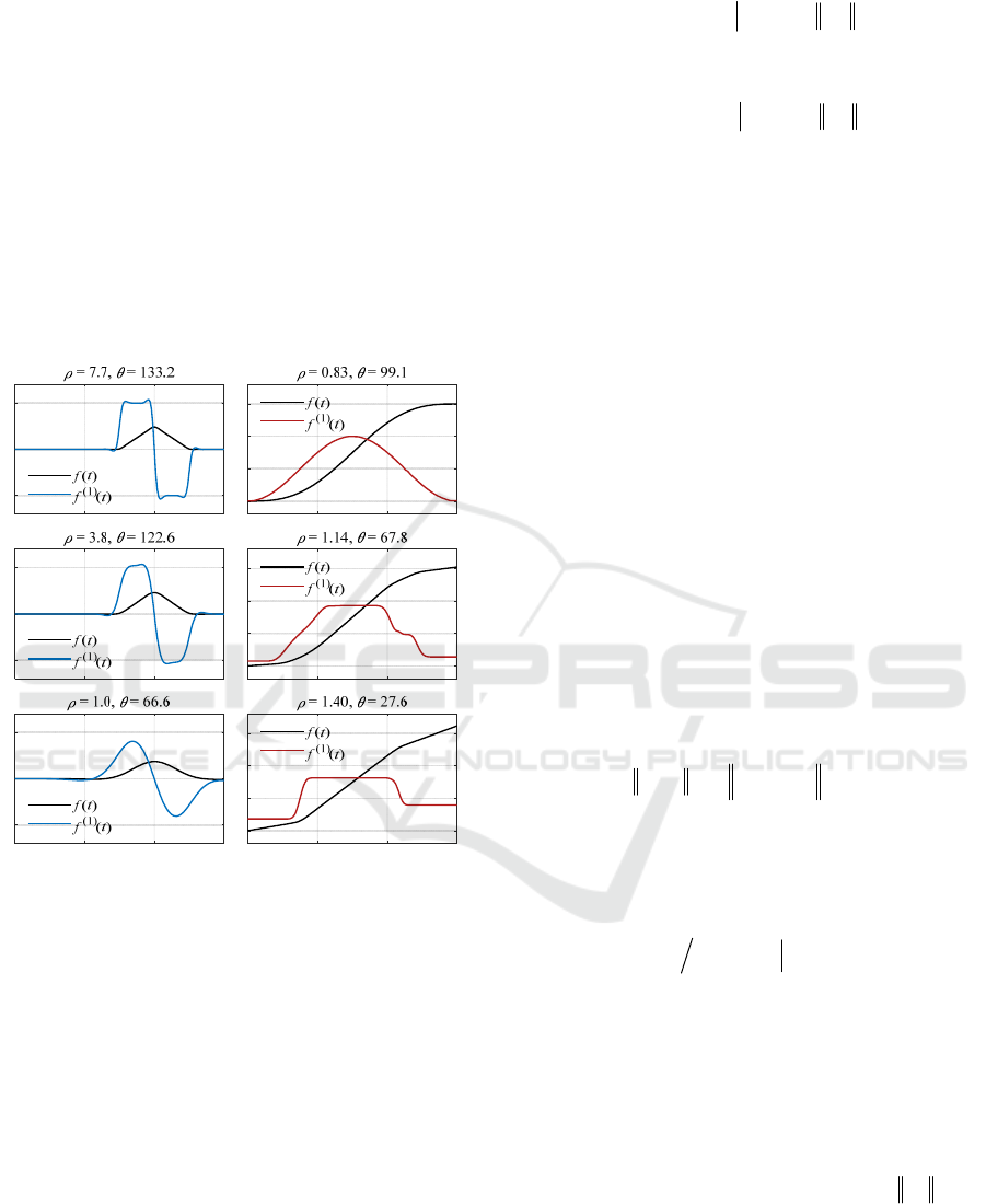
niques are illustrated in Figure 1, which presents the
shapes of some arbitrarily selected, exemplary func-
tions, characterised by different values of
and
.
Figure 1: Exemplary functions, characterised by different
values of
and
, together with their first derivatives;
the functions presented in the left column have been
obtained by imposing decreasing constraints on
(note
that
also decreases); the functions presented in the right
column have been obtained by imposing decreasing con-
straints on
(note that in this case
increases).
For practical choices of the constraints
max
and
max
, it is unlikely that there exists an admissible ap-
proximating function which satisfies such a constraint
and – at the same time – interpolates the measurement
data. Therefore, the vector of speed estimates needs
to be determined by minimising an indicator of the
fidelity of the results to the measurement data, denot-
ed hereinafter with
J
; in the case of Tikhonov regu-
larisation, this minimisation problem can be formu-
lated in the following way:
2
1
max
2
ˆ
arg inf ,
N
J
ξ
xξξDξR
(10)
and, analogously, in the case of TV regularisation:
2
1
max
1
ˆ
arg inf ,
N
J
ξ
xξξDξR (11)
Various choices for the indicator
J
are viable; the
one studied here is described in the next subsection.
2.3 Fusion of Data from Different
Sensors
In order to quantify the discrepancy between the
results of estimation and the measurement data, one
may evaluate the vector of approximation residuals,
computed in the following way:
1
ˆˆ
xx Qx x
(12)
The a priori information about the accuracy of the
employed sensors – the information contained in the
estimates
22
1
ˆˆ
,,
N
– can be incorporated in the
procedure for estimation of movement speed by al-
lowing for larger approximation residuals at the time
instants which correspond to the data acquired using
sensors with lower accuracy. This can be done by de-
fining the indicator
J
in Eq. (10) and Eq. (11) as a
weighted norm of the vector
ˆ
xx
, with weights se-
lected on the basis of the estimates
22
1
ˆˆ
,,
N
:
(13)
where
NN
W R
is a diagonal weighting matrix
whose nth element is defined as follows:
ˆˆ
max 1, ,
nn
wN
(14)
with
0
R
being a parameter controlling the
amount of weighting. For
0
, all the data are
taken into account with equal weights; for larger
,
the data corresponding to smaller
2
ˆ
n
(i.e. the data ac-
quired using more accurate sensors) have more influ-
ence on the estimates of speed. The division by the
maximum element in Eq. (14) ensures that
2
1
W
,
so that the values of
J
are in approximately the same
range regardless of the value of
.
The experiments described in Section 3 are aimed
at assessing the influence of the value of
and of
2
2
1
ˆˆ
J
W
W
xx Qx x
T
11
ˆˆ
Qx x W Qx x
Estimation of Movement Speed in Monitoring Systems based on Sensors of Multiple Types
73

the accuracy of the estimates
2
ˆ
n
on the quality of the
estimates of speed.
2.4 Computational Formulae
Equation (10), defining the vector of speed estimates
obtained using Tikhonov regularisation, can be
reformulated using the Lagrange multiplier technique
in the following way:
22
1
2
ˆ
arg inf
N
ξ
W
xQξxDξξ
R (15)
where
is a regularisation parameter (related to the
constraint
max
) whose value may be selected empi-
rically. The analytic solution of Eq. (15) yields:
1
1
TTT
ˆ
xQWQDDQWx
(16)
In the case of TV regularisation, the correspond-
ing minimisation problem – defined by Eq. (11) – can
be reformulated in an analogous way, viz.:
22
1
1
ˆ
arg inf
N
ξ
W
xQξxDξξ
R (17)
but the dependence of
1
ˆ
x
on
x
cannot be ex-
pressed in closed form, because the term
2
1
D
ξ
is not
differentiable. However,
1
ˆ
x
can be determined us-
ing the following iterative algorithm, being a general-
ised version of the algorithm described in (Chartrand,
2011) (which corresponds to
W
being the identity
matrix):
T
1
0
ˆ
00
x
(18)
11 1
1
ˆˆ ˆ
ii i
xx x
for
0,1, 2,i
(19)
where
1
ˆ
i
x
is the solution of the following set of
linear algebraic equations:
1
ˆ
ii
Hx g
(20)
TT
ii
HQWQ DED
(21)
11
TT
ˆˆ
ii ii
gQWQx x DEDx
(22)
with
11NN
i
E R
being a diagonal matrix whose
nth element is defined as follows:
(23)
1
The value of the regularisation parameter may significant-
ly influence the quality of the estimates of speed; however,
the problem of its selection remains outside the scope of this
The term 0𝜀≪1 is introduced to prevent the di-
vision by zero, whereas
is a regularisation param-
eter – related to the constraint
max
– whose value
may be selected empirically
1
.
3 NUMERICAL EXPERIMENTS
3.1 Methodology of Experimentation
The synthetic data, used for experimentation, have
been generated according to the formula:
for ,
(24)
an
d
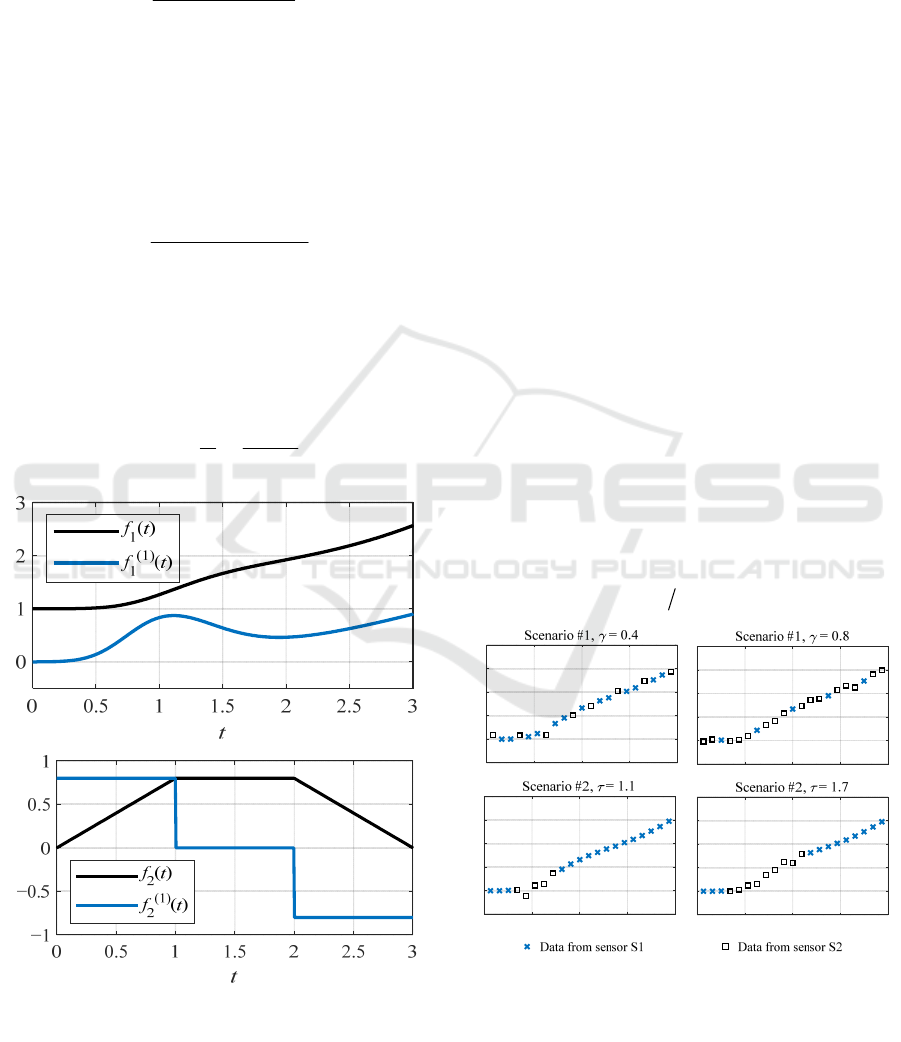
where:
12
6
3
3
21
1
3330
1exp
t
f
tt
for
0,3t
is a smooth test function, well suited to be differ-
entiated using Tikhonov regularisation;
2
0.8 for 1
0.8 for 1 2
0.8 3 for 2
tt
ft t
tt
is a piecewise-linear test function, better suited to
be differentiated using TV regularisation;
1
n
tn t
for
1, , 51nN
,
0.06t
,nr
x
are pseudorandom numbers following zero-
mean normal distributions whose variances are
2
n
;
R
is the number of generated sequences of syn-
thetic data, each corresponding to a different set
of pseudorandom numbers
,nr
x
for
1, ,nN
and
1, ,rR
.
The functions
1
f
and
2
f
, together with their first
derivatives:
12
65
1
2
33
1
1
3310
16 exp
tt
f
tt
(25)
1
2
0.8 for 1
0for1 2
0.8 for 2
t
ft t
t
(26)
are depicted in Figure 2.
paper. The interested reader may refer to, e.g., (Hansen,
2010, Chapter 5), (Bauer and Lukas, 2011) and (Reichel
and Rodriguez, 2013).
,
2
11
,1 ,
1
ˆˆ
in
in in
e
xx
,,nr k n nr
x
ft x
1, ,nN
1, ,rR
1, 2k
BIOSIGNALS 2021 - 14th International Conference on Bio-inspired Systems and Signal Processing
74
The level of disturbances in the data has been
characterised by the signal-to-noise ratio, defined in
the following way:
(27)
fo
r
The signal-to-noise ratio corresponding to the esti-
mates of the derivative
1
,
ˆ
nr
x
has been determined in
the analogous way:
(28)
fo
r
The performance of the studied methods of numerical
differentiation has been compared in terms of the
relative signal-to-noise ratio, defined as:
1,
1
0,
1
R
r
r
r
SNR
RSNR
RSNR
(29)
Figure 2: Functions used for the generation of synthetic data
and their first derivatives.
The numerical experiments have been designed in
such a way as to emulate a monitoring system em-
ploying two sensors – called S1 and S2 hereinafter –
which provide position estimates corrupted with er-
rors whose variances are
S1
and
S2
, respectively,
such that:
S2 S1
with
1, 10
(30)
Two scenarios have been considered:
According to the first one – called scenario #1
hereinafter – S1 and S2 are acquiring data simul-
taneously; approximately
N
data points, uni-
formly distributed over the time interval under an-
alysis, with
0.4,0.8
, are acquired by means
of S2, whereas the remaining data – by S1.
According to the second one – called scenario #2
hereinafter – S2 is only acquiring data for
0.5,t
, with
1.1, 1.7
, and S1 – only dur-
ing the remaining fragments of the time interval
under analysis. This scenario corresponds to the
configuration in which a sensor with low accuracy
is used only when the monitored person is outside
the field of view of another, more accurate sensor.
Exemplary data, generated according to both above-
described scenarios, are shown in Figure 3.
The sequences
1, ,
,,
rNr
x
x
have been normal-
ised in order to ensure that
0,r
SNR
remains approxi-
mately constant throughout the experimentation, re-
gardless of the ratio
S2 S1
:
Figure 3: Exemplary data generated according to scenario
#1 (first row) and scenario #2 (second row) for different
values of
and
.
2
1
0, 10
2
,
1
10log
N
n
n
r
N
nr n
n
ft
SNR
xft
1, ,rR
2
1
1
1, 10
2
11
,
1
10log
ˆ
N
n
n
r
N
nr n
n
ft
SNR
xft
1, ,rR
Estimation of Movement Speed in Monitoring Systems based on Sensors of Multiple Types
75

with
(31)
fo
r
The value
c
0.021
results in
0,
30
r
SNR
and is
roughly consistent with the authors’ previous experi-
ences with impulse-radar sensors and depth sensors
(Wagner et al., 2017).
It has been assumed that
S1
is known accurately,
i.e. that its perfect estimate
S1 S1
ˆ
is available; on
the other hand, the uncertainty of the estimate
S2
ˆ
of
S2
has been modelled in the following way:
S2 S2
ˆ
,
0.1, 10
(32)
For both test functions
1
f
and
2
f
and for both
scenarios, the following experiments have been per-
formed:
experiments aimed at assessing the influence of
the weighting of data on the quality of the speed
estimates for different ratios
S1 S2
, with
S1
and
S2
being known perfectly and the values of
all other parameters having been fixed;
experiments aimed at assessing the influence of
the weighting of data on the quality of the speed
estimates for different fractions of the data having
been acquired by means of sensor S2, with
S1
and
S2
being known perfectly and the values of
all other parameters having been fixed;
experiments aimed at assessing the influence of
the ratio
S1 S2
on the quality of the speed esti-
mates for different fractions of the data having
been acquired by means of sensor S2, with
S1
and
S2
being known perfectly and the values of
all other parameters having been fixed;
experiments aimed at assessing the influence of
the error corrupting the estimate
S2
ˆ
of
S2
on
the quality of the speed estimates for different
ratios
S1 S2
, with the values of all other param-
eters having been fixed.
The sequences of data, generated using the test
function
1
f
, have been differentiated using Tikhonov
regularisation, whereas those generated using the test
function
2
f
– using TV regularisation; such a choice
is justified by the shapes of those functions. For each
sequence of data, the value of the regularisation pa-
rameter
has been selected in such a way as to max-
imise RSNR; it is only possible in the synthetic setting
of the numerical experiments reported here. This pos-
sibility has been exploited in order to study the influ-
ence of other parameters on the quality of the speed
estimates independently from the influence of the re-
gularisation parameters, although – in practice – the
optimisation of regularisation parameters is an impor-
tant and complex task which, nevertheless, remains
outside the scope of this paper.
3.2 Results of Experiments
Figures 4–7 present the results of the numerical
experiments described in the previous subsection. In
order to facilitate the interpretation of these figures,
the symbols of selected parameters, together with
their descriptions, are collected in Table 1. The ob-
tained results indicate that:
The studied method for weighting the data on the
basis of the available information about the vari-
ances of errors corrupting those data yields an
improvement in the quality of the speed estimates
when the ratio
S2 S1
is sufficiently large, viz.
larger than ca. 2 (cf. Figure 4); when that ratio is
smaller, the use of
0
does not yield any sig-
nificant benefit.
The weighting of data is more advantageous in the
case of scenario #2 – i.e., when less accurate data
are acquired within a continuous fragment of the
time interval under analysis – than in the case of
scenario #1 – i.e., when less accurate data are
mixed uniformly with more accurate data (cf.
Figure 4, note the differences in the colour scales).
In most cases, the values provide the
best results (cf. Figure 4).
In the case of scenario #1, setting too large
yields only modest negative effects (cf. Figure 4,
left column). On the other hand, in the case of
scenario #2, setting too large may yield results
worse than setting – i.e., ignoring the
available information about the ratio (cf.
Figure 4, right column).
In the case of scenario #2, the dependencies of the
quality of the speed estimates on and on
are not significantly affected by the length of the
time interval in which the data are acquired by
sensor S2 (cf. the right columns of Figure 5 and
Figure 6).
In the case of scenario #1 with test function ,
no systematic dependency of the quality of the
speed estimates on the fraction of data acquired
2
2
,c
1
N
nr
n
x
N
c
0.021
1, ,rR
1, 3
0
S1 S2
2
f
BIOSIGNALS 2021 - 14th International Conference on Bio-inspired Systems and Signal Processing
76
using sensor S2 can be observed in the obtained
results (cf. the lower-left panels of Figure 5 and
Figure 6).
The quality of the speed estimates is sensitive to
the error corrupting the estimate of the variance
. In the case of scenario #1 with test function
, overestimation of that variance does not in-
crease the errors corrupting the speed estimates as
much as its underestimation. On the other hand, in
all the other cases, for larger values of that vari-
ance the best results are obtained, surprisingly,
when it is slightly underestimated (cf. Figure 7).
The results presented here are representative ex-
amples of the results of a more exhaustive set of ex-
periments, in which other values of the fixed param-
eters have also been taken into account.
Table 1: Symbols and descriptions of parameters presented
in Figures 4–7.
Symbol Description
the amount of weighting of the data according to the
estimates of the sensors’ accuracy; cf. Eq. (14) in
Subsection 2.3
in scenario #1, the fraction of the data acquired using
sensor S2; cf. Subsection 3.1
in scenario #2, the end of the time interval in which data
have been acquired using sensor S2; cf. Subsection 3.1
the ratio ; cf. Subsection 3.1
the relative error corrupting the estimate of ;
cf. Eq. (32) in Subsection 3.1
RSNR
the signal-to-noise ratio in the speed estimates, relative
to the signal-to-noise ratio in the measurement data; cf.
Eq. (29) in Subsection 3.1
Figure 4: Dependence of RSNR on
and
for both scenarios, both test functions and fixed values of
,
and
.
Figure 5: Dependence of RSNR on
and
or
for both scenarios, both test functions and fixed values of
and
.
2
S2
1
f
S2 S1
S2
ˆ
S2
Estimation of Movement Speed in Monitoring Systems based on Sensors of Multiple Types
77
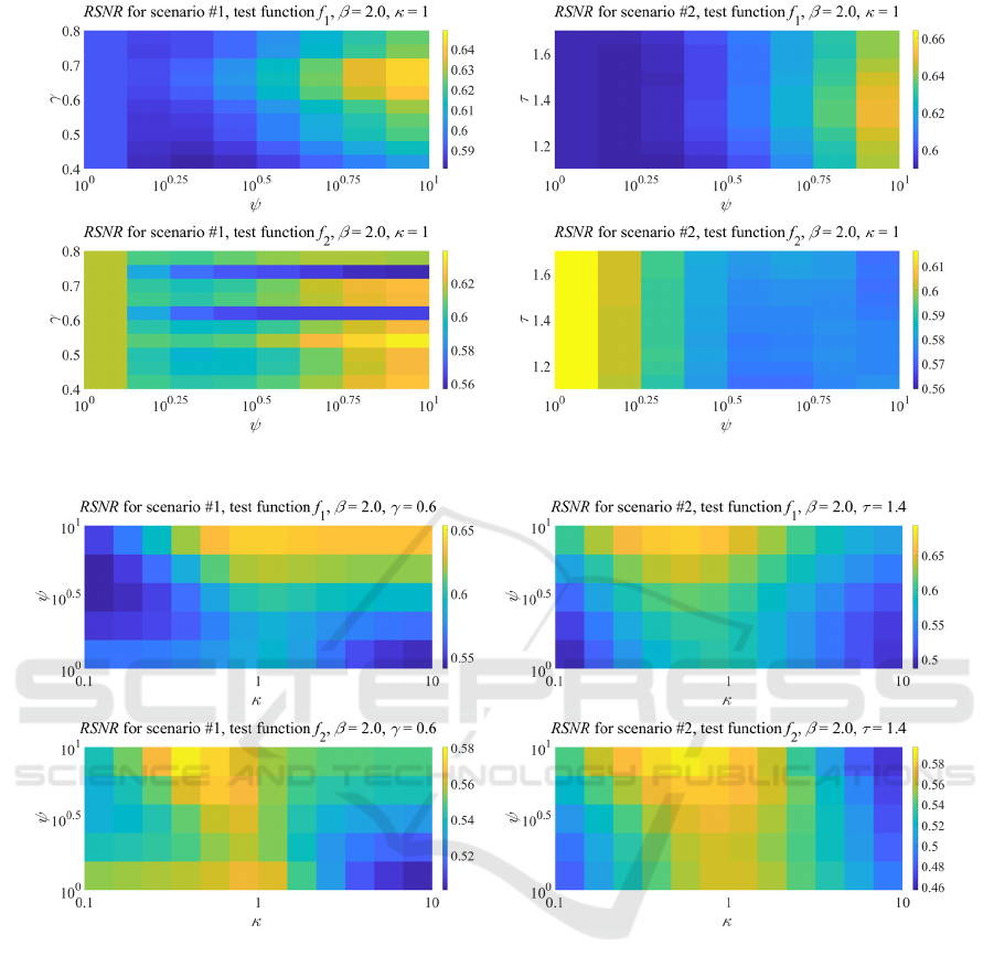
Figure 6: Dependence of RSNR on and or for both scenarios, both test functions and fixed values of and .
Figure 7: Dependence of RSNR on and for both scenarios, both test functions and fixed values of , and .
4 SUMMARY
AND CONCLUSIONS
Healthcare-oriented monitoring systems based on the
fusion of data from sensors of various types, which
allow for estimating the monitored person’s move-
ment speed, may assist healthcare practitioners in
their efforts to ensure good quality of life of elderly
persons and can contribute to the reduction of the
public expenditures related to the healthcare services
addressed to those persons.
The technique for fusion of measurement data ac-
quired by means of different sensors, presented in this
paper, may be used for improving the accuracy of the
estimates of speed obtained using such systems when
some a priori information about those data is avail-
able. Guidelines on the selection of the parameters
characterising that technique, based on numerical ex-
perimentation, are also provided. These results may
turn out to be useful in the development of monitoring
systems based on depth sensors and impulse-radar
sensors.
The prospects for future studies involve – above
all – experiments aimed at testing the described meth-
ods on the basis of real-world data.
BIOSIGNALS 2021 - 14th International Conference on Bio-inspired Systems and Signal Processing
78

ACKNOWLEDGEMENT
The work reported in this paper has been
accomplished within the project 2017/25/N/ST7/
00411 financially supported by the National Science
Centre, Poland.
REFERENCES
Al-Shaqi, R., M. Mourshed and Y. Rezgui, 2016. Progress in
ambient assisted systems for independent living by the
elderly. SpringerPlus, vol. 5, no. 1, p. 624.
Baldewijns, G., et al., 2016. Automated in-home gait transfer
time analysis using video cameras. Journal of Ambient
Intelligence and Smart Environments, vol. 8, no. 3, pp.
273–286.
Bauer, F. and M. A. Lukas, 2011. Comparing parameter
choice methods for regularization of ill-posed problems.
Mathematics and Computers in Simulation, vol. 81, no.
9, pp. 1795–1841.
Campos, W., A. Martinez, W. Sanchez, H. Estrada, N. A.
Castro-Sánchez and D. Mujica, 2016. A systematic
review of proposals for the social integration of elderly
people using ambient intelligence and social networking
sites. Cognitive Computation, vol. 8, no. 3, pp. 529–542.
Chartrand, R., 2011. Numerical differentiation of noisy,
nonsmooth data. ISRN Applied Mathematics, vol. 2011,
pp. 1–11.
Debes, C., A. Merentitis, S. Sukhanov, M. Niessen, N.
Frangiadakis and A. Bauer, 2016. Monitoring activities
of daily living in smart homes: understanding human
behavior. IEEE Signal Processing Magazine, vol. 33, no.
2, pp. 81–94.
Fleming, J. and C. Brayne, 2008. Inability to get up after
falling, subsequent time on floor, and summoning help:
prospective cohort study in people over 90. BMJ, vol.
337, p. a2227.
Garcia Marin, J., 2015. The use of interactive game
technology to improve the physical health of the elderly:
a serious game approach to reduce the risk of falling in
older people. Ph.D. thesis, Faculty of Engineering and
Information Technology, University of Technology,
Sydney.
Hagler, S., D. Austin, T. L. Hayes, J. Kaye and M. Pavel,
2010. Unobtrusive and ubiquitous in-home monitoring: a
methodology for continuous assessment of gait velocity
in elders. IEEE Transactions on Biomedical
Engineering, vol. 57, no. 4, pp. 813–820.
Hansen, P. C., 2010. Discrete Inverse Problems: Insight and
Algorithms, Society for Industrial and Applied
Mathematics.
Hodgins, D., 2008. The importance of measuring human gait.
Medical Device Technology, vol. 19, no. 5, pp. 42–47.
Khan, S. S. and J. Hoey, 2017. Review of fall detection
techniques: a data availability perspective. Medical
Engineering and Physics, vol. 39, pp. 12–22.
Kikkert, L. H. J., N. Vuillerme, J. P. van Campen, T.
Hortobágyi and C. J. Lamoth, 2016. Walking ability to
predict future cognitive decline in old adults: a scoping
review. Ageing Research Reviews, vol. 27, pp. 1–14.
Lusardi, M., 2012. Is walking speed a vital sign? Topics in
geriatric rehabilitation, vol. 28, no. 2, pp. 67–76.
Majumder, S., et al., 2017. Smart homes for elderly
healthcare—recent advances and research challenges.
Sensors, vol. 17, no. 11, p. 2496.
United Nations, Department of Economic and Social Affairs,
Population Division, 2019. World population prospects
2019: Highlights. ST/ESA/SER.A/423. Available:
https://population.un.org/wpp/publications (as of
October 5, 2020).
Peetoom, K. K. B., M. A. S. Lexis, M. Joore, C. D. Dirksen
and L. P. De Witte, 2015. Literature review on
monitoring technologies and their outcomes in
independently living elderly people. Disability and
Rehabilitation: Assistive Technology, vol. 10, no. 4, pp.
271–294.
Reichel, L. and G. Rodriguez, 2013. Old and new parameter
choice rules for discrete ill-posed problems. Numerical
Algorithms, vol. 63, no. 1, pp. 65–87.
Rudin, L. I., S. Osher and E. Fatemi, 1992. Nonlinear total
variation based noise removal algorithms. Physica D:
Nonlinear Phenomena, vol. 60, no. 1, pp. 259–268.
Sharkey, A. and N. Sharkey, 2012. Granny and the robots:
ethical issues in robot care for the elderly. Ethics and
Information Technology, vol. 14, no. 1, pp. 27–40.
Shumway-Cook, A., S. Brauer and M. Woollacott, 2000.
Predicting the probability for falls in community-
dwelling older adults using the Timed Up & Go test.
Physical Therapy, vol. 80, no. 9, pp. 896–903.
Stickel, J. J., 2010. Data smoothing and numerical
differentiation by a regularization method. Computers &
Chemical Engineering, vol. 34, no. 4, pp. 467–475.
Wada, K., T. Shibata, T. Saito and K. Tanie, 2004. Effects of
robot-assisted activity for elderly people and nurses at a
day service center. Proceedings of the IEEE, vol. 92, no.
11, pp. 1780–1788.
Wagner, J., et al., 2017. Comparison of two techniques for
monitoring of human movements. Measurement, vol.
111, pp. 420–431.
World Health Organization, 2017. Integrated care for older
people: guidelines on community-level interventions to
manage declines in intrinsic capacity. Available:
https://apps.who.int/iris/handle/10665/258981 (as of
June 14, 2019).
Estimation of Movement Speed in Monitoring Systems based on Sensors of Multiple Types
79
