
Visual-based Global Localization from Ceiling Images using
Convolutional Neural Networks
Philip Scales
1
, Mykhailo Rimel
2
and Olivier Aycard
1
1
LIG-MARVIN, Université Grenoble Alpes, 621 Avenue Centrale, Saint-Martin-d'Hères, France
2
Department of Computer science, Grenoble INP, 46 Avenue Félix Viallet, Grenoble, France
Keywords: Visual-based Localization, CNN, Mobile Robot.
Abstract: The problem of global localization consists in determining the position of a mobile robot inside its
environment without any prior knowledge of its position. Existing approaches for indoor localization present
drawbacks such as the need to prepare the environment, dependency on specific features of the environment,
and high quality sensor and computing hardware requirements. We focus on ceiling-based localization that is
usable in crowded areas and does not require expensive hardware. While the global goal of our research is to
develop a complete robust global indoor localization framework for a wheeled mobile robot, in this paper we
focus on one part of this framework – being able to determine a robot’s pose (2-DoF position plus orientation)
from a single ceiling image. We use convolutional neural networks to learn the correspondence between a
single image of the ceiling of the room, and the mobile robot’s pose. We conduct experiments in real-world
indoor environments that are significantly larger than those used in state of the art learning-based 6-DoF pose
estimation methods. In spite of the difference in environment size, our method yields comparable accuracy.
1 INTRODUCTION
Localization is essential for any autonomous or semi-
autonomous mobile robot. A robot must know its
pose relative to the environment to make decisions,
move or perform actions. In a broad sense, the goal of
localization is to provide the robot's pose. It can be a
pose in the world, in a specific environment or with
respect to another object. For global localization, the
robot must determine its pose without any prior
assumptions, enabling it to solve the Kidnapping
problem. As interest in social robotics rises, we are
seeing robots deployed in hospitals, malls, care
homes, and other populated indoor environments. We
consider the problem of globally localizing the robot
within crowded indoor environments.
Different sensors can be used to estimate motion
and/or acquire observations, the most frequently used
being laser range finders (LRFs) and cameras.
However, all sensors have their limitations, usually
making them applicable only in certain conditions
and/or environments. When using LRFs in crowded
environments, a large proportion of laser hits will
provide distances to people which is not relevant for
localization. Furthermore, laser range finders are
orders of magnitude more expensive than cameras.
There are also a number of solutions requiring some
modification of the environment, such as setting up
wireless beacons, or installing artificial landmarks
and visual features. We aim to avoid modifying the
environment, since this may not be possible, or may
be too costly in some real-world applications. When
solving a localization problem, the map of the
environment may or may not be given as input. If the
map is not given, the problem is Simultaneous
Localization and Mapping (SLAM) (Bailey and
Durrant-Whyte, 2006), which we don’t consider.
We aim to develop a real-time framework for the
indoor global localization of a wheeled mobile robot,
which can be applied in crowded environments with
varying lighting conditions. As a first step towards a
complete framework, in this paper, we provide a
method for estimating the robot’s pose from a single
ceiling image. This method can be used with mid-
range, relatively low-cost hardware. Additionally, our
method is straightforward to implement, and all its
dependencies are open-source software. We propose
to use a supervised learning approach —
Convolutional Neural Networks (CNNs) — to
estimate the robot’s 2-DoF position and orientation
angle from a single ceiling image taken by a fisheye
camera mounted on the robot.
Scales, P., Rimel, M. and Aycard, O.
Visual-based Global Localization from Ceiling Images using Convolutional Neural Networks.
DOI: 10.5220/0010248409270934
In Proceedings of the 16th International Joint Conference on Computer Vision, Imaging and Computer Graphics Theory and Applications (VISIGRAPP 2021) - Volume 5: VISAPP, pages
927-934
ISBN: 978-989-758-488-6
Copyright
c
2021 by SCITEPRESS – Science and Technology Publications, Lda. All rights reserved
927

2 RELATED WORK
Given the assumptions we made in the Introduction,
in this section we focus on the review of vision-based
methods for mobile robot localization. These methods
can vary depending on where the camera is mounted,
how features are extracted from the acquired images,
and in which environment the robot operates.
Some works (Jin and Lee, 2004; Delibasis et al.,
2015) use ceiling-mounted cameras to localize an
indoor mobile robot. The former uses neural networks
to detect a robot in an image and the latter uses
segmentation techniques with a robot marked with a
specific color. Front-facing cameras were used in
(Kendall et al., 2015; Kendall et al., 2017; Clark et al.,
2017; Brahmbhatt et al., 2018; Kendall et al., 2016)
to perform indoor and outdoor 6-DoF camera
relocalization. Although their task was not to localize
a mobile robot, their work is relevant. There are also
approaches for general place recognition (Zhang et
al., 2016) which do not provide sufficient accuracy
for robot localization. CNNs are useful in image
classification tasks since they are able to extract
features from images (Krizhevsky et al., 2012). The
CNN in (Kendall et al., 2015) is able to recognize
high-level features, such as building contours, and
learns the relation between those features and the
pose of the camera. This allows them to regress the 6-
DoF pose from an RGB image in real-time.
An alternative is to mount an upwards-facing
camera on top of the robot. We will refer to these as
ceiling-vision cameras, the first use of which was in
(King and Weiman, 1991). The earlier publications
relied on the presence of active lights on the ceiling
to perform localization, with (Thrun et al., 1999)
measuring the brightness of a local patch of the
ceiling above the robot. More approaches have been
developed since then including the use of artificial
markers (e.g. barcodes, April tags, infra-red beacons
etc.) (Nourbakhsh, 1998) and extracting primitives
(e.g. lines, corners etc.) (Jeong and Lee, 2005). In
(Thrun, 1998), ceiling-vision cameras and artificial
neural networks were used to recognize manually
defined high-level features. However, they used
individual networks for each feature, and their
experiments were limited to a corridor environment.
Approaches using a front-facing camera may fail
in situations where many dynamic obstacles obstruct
recognizable features of the environment. Our use of
a ceiling-vision camera aims to limit such
obstructions. Approaches using ceiling-mounted
cameras or artificial landmarks require the
environment to be modified, and the use of ceiling
lights is only feasible in environments where the
lights are constantly switched on. The use of
manually-defined high-level features makes it harder
to adopt the algorithm for various types of ceilings
composed of different types of panels or lamps.
There are a few fundamental differences between
the applications of our approach and those considered
for camera relocalization (Kendall et al., 2015;
Kendall et al., 2017; Clark et al., 2017; Brahmbhatt et
al., 2018; Kendall et al., 2016). These works obtained
high 6-DoF pose accuracy (0.18-0.48m, 0.11-
0.17rad) using the 7-Scenes dataset (Zhang et al.,
2016) which was acquired in small indoor
environments (2-12m², 1-1.5m height). They also
evaluate their methods in larger outdoor
environments (875-50000m²), but the accuracy
obtained is insufficient for indoor localization of a
mobile robot (1.46-3.67m, 0.13-0.25rad). In contrast,
we aim to provide accurate localization at any point
of rooms of around 100m². Furthermore, images of
ceilings generally contain less visual features than
images from outdoor or 7-scenes datasets. Finally,
these works do not evaluate the performance of their
networks on more constrained embedded hardware
typical for indoor mobile robots.
A more recent work (Xiao et al., 2019) explores
how to ignore dynamic objects when performing
visual SLAM using deep CNNs.
3 METHODS
3.1 Overview
We combine the use of a ceiling-vision camera and
CNNs to estimate the pose of a mobile robot. Our
ceiling-image localization module takes a single raw
camera image as input, and outputs the position [x,y]
and orientation θ of the robot in the frame of an
existing map of the environment. We motivate our
choices in section 3.2.
Our localization module operates in two steps. In
step one, an image of the ceiling is acquired using a
camera mounted on top of a robot. The raw camera
image is pre-processed as described in section 3.3. In
step two, the pre-processed image is used as the input
to two CNNs, which were separately trained to
predict robot position and orientation from a ceiling
image. Position and orientation predictions are
combined to form the 3-DoF pose prediction which is
directly used for robot localization. In the scope of
this work, we do not consider applying additional
filters or sensor fusion. The CNN architectures are
described in section 3.4. Details of dataset
construction are given in section 3.5. The steps for
VISAPP 2021 - 16th International Conference on Computer Vision Theory and Applications
928

localizing the robot are summarized in Fig. 1. Pseudo-
code for the pose update is provided in Fig. 2.
Figure 1: Summary of the localization module.
3.2 Motivation
CNNs learn which features are relevant to a given
dataset and task, so applying our method to a new
environment requires only a new dataset and network
training, as opposed to manual tweaking of pre-
defined features. Inspired by works in the field of
place recognition and 6-DOF camera relocalization,
we use CNNs to estimate the 3-DoF pose of the robot
from an image. CNNs for complex tasks have a high
memory and computational cost. We split the task
into the estimation of the 2-DoF position, and
estimation of the orientation, each of which is treated
as a regression problem solved by a separate CNN.
This was more accurate than using a single CNN with
our architecture to regress the full 3-DoF pose.
Using only a ceiling image as input allows our
approach to provide immediate global localization,
without the need for an external initial pose
estimation as input or environment exploration phase.
Input: cameraImage img
Output: pose p
Algorithm:
img ← receive_image()
img ← resize(img, 160, 120)
img ← convert_to_greyscale(img)
img ← apply_clahe(img)
p.position ←
position_cnn.predict(img)
p.orientation ←
orientation_cnn.predict(img)
publish_pose(p)
Figure 2: Pseudocode of one localization cycle.
3.3 Image Pre-Processing
The input images to the CNN are obtained by
applying a pre-processing step to the camera images;
they are resized to a resolution of 160x120 pixels,
converted to greyscale, and contrast-limited adaptive
histogram equalization (CLAHE) (Pizer et al., 1987)
is applied to them. The image resolution was chosen
as a trade-off between the localization accuracy, and
the size and computational requirements of the CNN.
We decided to disregard the color information
because there are few color features on most ceilings.
CLAHE was applied to make the network less
sensitive to changes in ambient lighting.
3.4 CNN Architectures
In order to design our CNN, we experimented with
various network architectures. We decided to use the
same base CNN architecture to construct our position
and orientation CNNs, with the only difference being
the number of outputs. We base our final architecture
on only a sub-part of the GoogLeNet architecture
(Szegedy et al., 2015) because our task is different,
and we target a lower computational cost.
Starting with the full GoogLeNet architecture, the
process to build our CNN can be summarized as
follows: (1) we took the first part of GoogLeNet
(from Input to Softmax0 layer in Fig. 3 of (Szegedy
et al., 2015)); (2) we adapted existing layers to suit
our dataset and task by modifying the input layer to
suit our images, and by adapting the output layer for
regression; (3) we added Batch Normalization layers
after the first two Maxpool layers; (4) we adjusted
network hyperparameters. In the rest of this section,
we detail our changes to the original GoogLeNet,
with all unmentioned aspects left unchanged.
GoogLeNet can be understood as having two
auxiliary classifiers branching off from the main
classifier at earlier stages. Generally speaking, in
CNNs, early layers close to the input learn filters that
capture low-level features, and later layers closer to
the output capture high-level features. Ceilings are
usually made up of many lower-level features, such
as lines, edges, lamps, exit signs, and ceiling panels.
In contrast, GoogLeNet was designed to classify
images into 1000 categories, each of which required
the network to capture high-level features. This
observation led us to make use of only the first
auxiliary classifier, discarding other layers. The layer
parameters such as number of units, number and size
of filters, and their structure were left unchanged.
We adapted the input layer to our data by
changing the input shape to 160x120x1(width, height,
channels) in order to suit our images, which are
smaller than those used in GoogLeNet, and use only
one color channel. Consequently, the sizes of our
feature maps are different, and can be seen in Fig. 3.
We adapted the output layer by replacing the
softmax0 with a dense layer with one or two units for
orientation or position regression respectively.
Batch normalization (Ioffe and Szegedy, 2015)
consists in normalizing the inputs of a layer for each
batch of images. This allows us to limit overfitting by
improving regularization, which is especially needed
when using small datasets such as ours. We
introduced Batch normalization layers after each of
the first two MaxPooling layers, as seen in Fig. 3.
Visual-based Global Localization from Ceiling Images using Convolutional Neural Networks
929
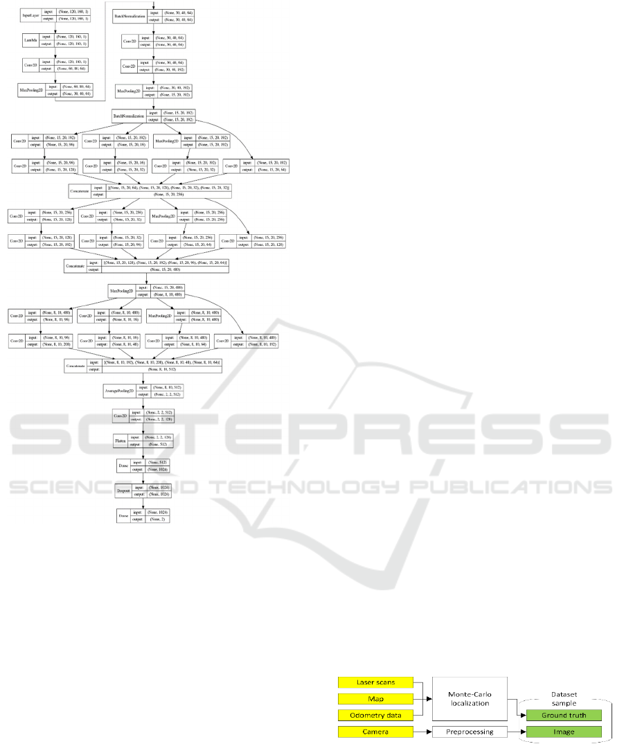
Figure 3: CNN for position regression with layer types and
feature map shapes (best viewed on the digital version).
Hyperparameters are tuned to maximize a
network’s performance on a given task and dataset.
We experimented with various parameters
considering what worked best for our task, datasets,
and hardware. We used the Amsgrad stochastic
gradient descent optimizer (learning rate=0.001,
beta1=0.9, beta2=0.999, epsilon=10⁻⁷, decay=0)
(Reddi et al., 2018). We reduced the batch size for
training from 256 to 16 to account for our dataset size,
which is smaller than GoogLeNet was designed for.
This also reduced the memory requirements when
training the network, allowing us to target mid-range
hardware. For the task of position estimation, we
augmented the dataset by applying random rotations
to the images. Given that our camera was centered on
the robot, this was equivalent to capturing images
from the same position at different orientations.
PoseNet (Kendall et al., 2015) and other similar
works perform 6-DoF camera relocalization in town-
scale outdoor, and room-scale indoor environments.
These environments contain many high-level features
which are useful for camera relocalization. Since they
deal with a less constrained problem and high-level
features, they use larger networks. Our approach is a
smaller architecture that still maintains sufficient
representation capacity for our task.
3.5 Dataset Construction
The dataset required to train the CNNs is built by
teleoperating the robot in the environment in which it
will be deployed, while acquiring images of the
ceiling along with the corresponding ground-truth
poses. The images are pre-processed as described in
section 3.3. The quality of the CNN’s predictions
depends on the dataset, which is affected by the
conditions in which the images are acquired, as well
as the method by which the ground-truth pose is
acquired. Artificial and natural lighting conditions
were varied during data acquisition to improve the
CNN’s robustness. For artificial lighting, data was
acquired with all lights on, or all lights off. The
ground-truth pose is provided by an alternative
existing localization method. We used laser-based
Adaptive Monte-Carlo Localization (AMCL) (Fox et
al, 1999) coupled with an existing map of the
environment to provide ground-truth measurements.
We acquired data in a quasi-static environment in
order to maximize the accuracy of the AMCL.
We discarded samples for which the ground-truth
localization had reported a high uncertainty, which
we defined as samples where any one of the pose
covariances were higher than a threshold: σ(x,x) >
0.15m² or σ(y,y) > 0.15m² or σ(θ,θ) > 0.1rad². This
does not eliminate the problem of the pose estimation
drifting out of accuracy as the robot is teleoperated.
To mitigate this effect, data acquisition was
performed by combining data from several shorter
acquisitions. Fig. 4 summarizes the data acquisition.
Figure 4: Overview of the data acquisition method.
VISAPP 2021 - 16th International Conference on Computer Vision Theory and Applications
930
4 EXPERIMENTAL SETUP AND
RESULTS
We implemented our method in order to deploy it on
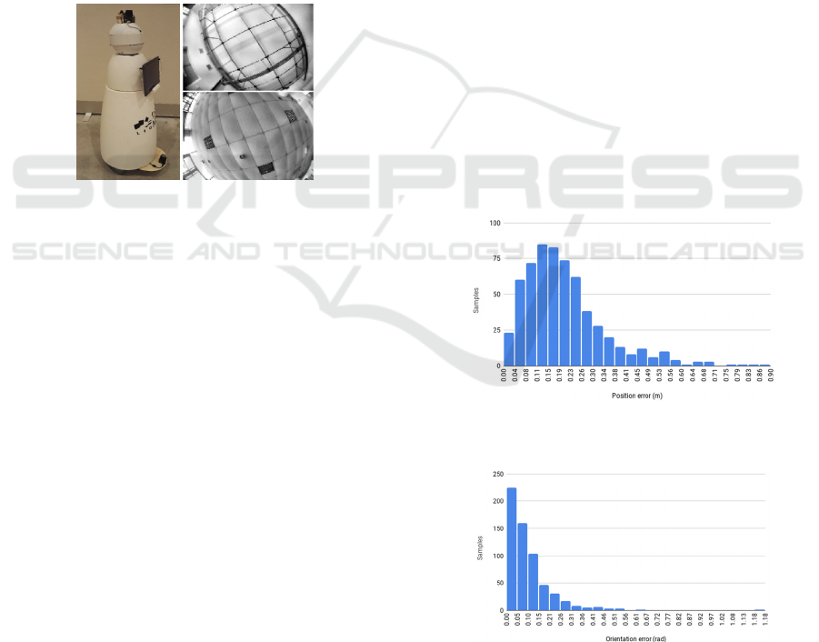
RobAIR (“RobAIR”) (see Fig. 5), a wheeled mobile
robot and tested it in real environments and situations.
In this section, we describe the hardware, software,
the experimental protocol, and results.
4.1 Environments and Datasets
We considered two environments (denoted as A and
B - see Fig. 5) with different ceiling features. Their
areas were 83 m² and 72 m², and ceiling heights of 4m
and 2.5m for A and B respectively. A dataset was
built for each environment by teleoperating the robot
at a speed of 0.5 m/s. Images were acquired at 5fps
and associated with their ground truth pose.
Figure 5: Left: RobAIR. Right: images of the ceiling in
environments A (top) and B (bottom).
For environment A, 30105 samples were acquired
(train, validation data split: 89.7%, 10.3%). For
environment B, 27237 samples were acquired (train,
validation split: 80.5%, 19.5%). We deployed the
robot in three test scenarios: (1) an uncrowded
environment; (2) an uncrowded environment with a
new artificial lighting configuration; (3) an
environment where several participants partially
obstructed the camera’s view. In order to evaluate the
performance of our approach, we teleoperated the
robot while recording samples composed of the
ceiling image, ground-truth pose, and our method’s
pose prediction. New samples were taken when the
ground-truth pose changed by more than 0.001m or
0.001rad in order to discard moments when the robot
was stationary. We present statistics on position and
orientation errors for the different scenarios in Table
1, computed using the testing datasets of 400 to 600
samples, acquired over 320 to 609 seconds.
4.2 Implementation Details
The camera we used was a low-resolution (640x480
pixels) USB camera, equipped with a fish-eye lens. It
was mounted on top of the RobAIR, at a height of
120cm. The robot was equipped with an i5-6200U
processor. The full pose estimation step took 100ms
to run on the robot’s processor. When performing
localization, the camera recorded at 5fps, hence the
pose update rate was 5Hz. We implemented the
localization module as a ROS node. CNNs were
implemented in Python using Keras with Tensorflow
backend. Training was performed on a mid-range
laptop GPU (Nvidia GTX 960m, 2GB of VRAM)
using CUDA. Networks were trained for 30 epochs
(about 1 hour each network). The laser for ground-
truth pose acquisition was a Hokuyo URG-04LX-
UG01 rangefinder, mounted on the base of RobAIR.
4.3 Experimental Results and Analysis
In Fig. 6 and Fig. 7, we show the histograms of pose
error values for scenario 1, environment B. The
supplementary video contains a visualization of the
pose predictions in our evaluation scenarios, as well
as the graphs of errors over the whole duration of each
scenario, which give an idea of how the pose
prediction behaves over time. For both position and
orientation, the general trend in error values varies
according to which part of the environment the robot
is in. Error values fluctuate continuously during the
evaluation, with occasional large error spikes. In all
scenarios, the error behaves in a similar fashion.
Figure 6: Position estimation error histogram for scenario 1
in environment B (609 samples).
Figure 7: Orientation error histogram for scenario 1 in
environment B (609 samples).
Scenario 1 consisted in sampling the data from
the testing datasets used to evaluate the CNNs. These
Visual-based Global Localization from Ceiling Images using Convolutional Neural Networks
931
datasets were acquired in environments with lighting
conditions that the network had trained on (all lights
on or all off). The number of dynamic obstacles in the
environments was negligible, so that ground-truth
laser-based localization would not be affected. The
camera’s view of the ceiling was not obstructed by
people or other dynamic obstacles. This scenario was
performed in environments A and B. The accuracy of
the localization in this scenario demonstrates the
viability of our approach.
Scenario 2 consisted in sampling the data from
environment A while changing the artificial lighting
conditions. During this scenario, we used lighting
configurations where a subset of the lights was
switched on. The training dataset for the CNNs did
not contain this lighting configuration. While the
accuracy of the localization is worse than with all
lights on or off, our approach manages to produce a
relatively stable localization. We also note that often,
large spikes in pose error occur as the lights were
switched on/off, probably due to the camera’s built-
in brightness adaptation.
Table 1: Error of our approach relative to ground-truth.
Scenario
and env.
Pose estimation error
Average
and 95%
confidence
interval
Standard
deviation
Max
1A
0.17±0.01m
0.13±0.02rad
0.12m
0.17rad
0.73m
1.60rad
1B
0.21±0.01m
0.10±0.01rad
0.14m
0.11rad
0.87m
1.18rad
2A
0.60±0.09m
0.32±0.05rad
0.87m
0.53rad
6.58m
3.03rad
3B
1.57±0.13m
0.26±0.02rad
1.57m
0.24rad
7.13m
2.20rad
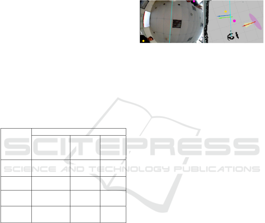
Scenario 3 consisted in sampling the data from
environment B while several people were present.
People were instructed to walk or stand within 3m of
the robot. This led to the robot’s view of the ceiling
being partially obstructed by people’s faces and upper
body. As a reminder, our network never trained on
such conditions. Error for both position and
orientation spiked when large parts of the ceiling
were obstructed. Laser-based AMCL occasionally
drifted, providing highly inaccurate pose estimations,
an example of which is given in Fig. 8.
Orientation error behaved similarly to scenario 1,
albeit with a slightly higher average error. Position
error averaged above 3m for more than 30
consecutive samples three times, all in similar areas
of the environment. To visualize which parts of the
image influenced the CNN output, we generated
activation heatmaps for a high-error sample from
scenario 3 and a low-error sample from a similar
position in scenario 1 (see Fig. 9).
Figure 8: Left:camera image. Right: top-down view of the
map (cells are 1m²). The vertical cyan line serves as a
reference between the image and map. Arrows: actual robot
position observed by the experimenter (green), our method
(blue), laser-based amcl (red, with position and orientation
uncertainties). Yellow and pink dots represent people.
We observe two differences between scenarios 1
and 3: (1) the combination of the pillar and lights in
the top right corner of the image is a distinctive
feature of this area, and it was blocked by a person in
scenario 3. This may explain activation differences
seen in row 1 Fig. 9. (2) The lights in the corridor in
the bottom left corner were always switched off
during training and in scenario 1, whereas they were
on for scenario 3. This may explain the activation
differences in rows 2 and 3 of Fig. 9. For orientation,
the heatmaps were very similar except for the corridor
area, which may explain the comparatively low error.
5 DISCUSSION
As with any supervised learning approach, we are
highly dependent on the quality of the dataset.
Acquiring ground truth data for the CNNs proved
difficult, due to inaccuracies in the laser-based
localization. There would be room for improvement
if a more reliable ground truth method were used.
In order to deploy a robot using our method, one
still needs to spend a fair amount of time acquiring
the dataset and ensuring coverage of the whole
environment, although this process could be
automated with an environment exploration
algorithm. Acquiring ground-truth supposes that one
has access to an alternative method for localization,
potentially requiring more expensive sensors.
However, once the dataset has been acquired by a
single robot, our method can be deployed on any
number of robots using a simple inexpensive camera.
VISAPP 2021 - 16th International Conference on Computer Vision Theory and Applications
932
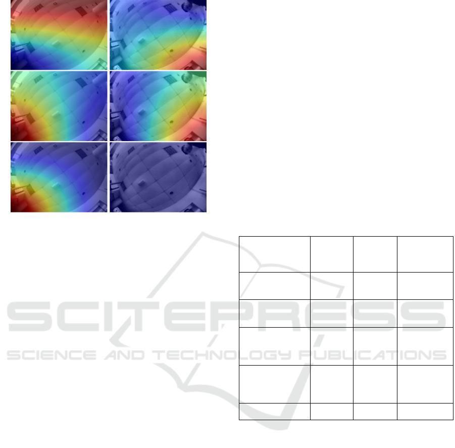
Figure 9: Comparison of position CNN output activation
heatmaps generated using Keras-vis grad-cam (“keras-
vis”), overlayed on the pre-processed image. Left to right:
scenarios 1, 3. Top to bottom: heatmaps for areas that
decrease, maintain, and increase the output values
corresponding respectively to the “grad_modifier”
parameters negate, small_values, and None. The
“backprop_modifier” parameter was None.
Using the raw network predictions directly as the
robot’s pose is currently unstable. The network
occasionally outputs a pose with high error. This
could be due to specific areas in the environment
where the ceiling is too similar to another location.
The accuracy loss when dealing with partial
obstruction of the image by people could be reduced
by mounting the camera higher on the robot, or
potentially by using a fish-eye lens with less
deformation. Further experiments would need to be
conducted in truly crowded scenarios to confirm this.
Table 2 shows average position and orientation
errors from recent 6-DoF camera relocalization works
using the 7-scenes dataset where environments have
an average size of 13 m
3
. While our work solves for
the 3-DoF case, our test scenarios cover much larger
environments, often with fewer distinctive features.
Although the applications of our approach (3-DoF
indoor robot localization) are different that the ones
in the related works (6-DoF camera relocalization) we
find it beneficial to provide such a comparison.
6 CONCLUSION
This work serves as an exploration into an original
solution to global localization of a mobile robot in
indoor environments. We have detailed a method to
learn the correspondence between images of the
ceiling and the robot’s position and orientation using
a supervised learning approach (CNNs).
Our method was tested in two real environments
with areas of around 72m² and 80m², with average
position and orientation errors in the order of 0.19m
and 0.11rad (median 0.16m, 0.07rad) in uncrowded
environments. These results indicate that our method
has some potential, especially considering the modest
hardware requirements in terms of sensors and
processing power. Tests were performed with varied
artificial lighting conditions where our method
showed some degree of robustness to lighting
changes. Partial obstruction of the ceiling images by
people standing near the robot led to significantly
higher errors in position estimation, and a relatively
small increase in orientation estimation errors.
Table 2: Comparison to 6-DoF camera relocalization work.
Approach Dataset
Median
position
error
Median
orientation
error
VIDLOC (Clark
et al., 2017)
7-scenes 0.26m N/A
PoseNet (Kendall
et al., 2015)
7-scenes 0.48m 0.17rad
MapNET
(Brahmbhatt et al.,
2018)
7-scenes 0.20m 0.11rad
MapNET PGO
(Brahmbhatt et al.,
2018)
7-scenes 0.18m 0.11rad
Ours Scenario 1 0.16m 0.07rad
7 FUTURE WORK
In order to better deal with crowded environments, a
training dataset could be acquired when people are
present in the environment. Such a dataset would
potentially be harder to acquire; however, the
network should be able to provide better localization
than when trained on a dataset of a static
environment. The existing dataset could be modified
by adding people at random locations in the images.
In order to incorporate this work into a complete
localization framework, we can filter the output of the
pose prediction networks to provide a more stable
estimate. One could also consider a set of poses over
time in order to discard outliers. The stable pose
Visual-based Global Localization from Ceiling Images using Convolutional Neural Networks
933

estimation can be combined with other localization
data such as odometry using sensor fusion.
The speed of the pose update could be improved
by adopting a more elaborate CNN architecture.
Recent CNN architectures can minimize resource
usage while maintaining good accuracy for their tasks
(Zhang et al., 2018). Further experimentation with
architectures and hyper parameters could also
improve accuracy and inference time.
ACKNOWLEDGEMENTS
This work has been partially supported by MIAI @
Grenoble Alpes, (ANR-19-P3IA-0003).
REFERENCES
Brahmbhatt, S., Gu, J., Kim, K., Hays, J., & Kautz, J.
(2018). Geometry-aware Learning of Maps for camera
localization. 2018 IEEE/CVF Conference on Computer
Vision and Pattern Recognition, 2616–2625.
Burgard, W., Cremers, A. B., Fox, D., Hähnel, D., Thrun,
S., Dellaert, F., Bennewitz, M., Rosenberg, C., Roy, N.,
Schulte, J., & Schulz, D. (1999). MINERVA: A second
generation mobile tour-guide robot. Proceedings of the
IEEE International Conference on Robotics and
Automation (ICRA).
Clark, R., Wang, S., Markham, A., Trigoni, N., & Wen, H.
(2017). Vidloc: A deep spatio-temporal model for 6-dof
video-clip relocalization. 2017 IEEE Conference on
Computer Vision and Pattern Recognition (CVPR),
2652–2660.
Delibasis, K. K., Plagianakos, V. P., & Maglogiannis, I.
(2015). Estimation of robot position and orientation
using a stationary fisheye camera. International
Journal on Artificial Intelligence Tools, 24(06),
1560004.
Dellaert, F., Fox, D., Burgard, W., & Thrun, S. (1999).
Monte Carlo localization for mobile robots.
Proceedings 1999 IEEE International Conference on
Robotics and Automation (Cat. No.99CH36288C), 2,
1322–1328.
Durrant-Whyte, H., & Bailey, T. (2006). Simultaneous
localization and mapping: Part I. IEEE Robotics &
Automation Magazine, 13(2), 99–110.
Ioffe, S., & Szegedy, C. (2015). Batch Normalization:
Accelerating Deep Network Training by Reducing
Internal Covariate Shift. Proceedings of the 32nd
International Conference on Machine Learning.
Jeong, W., & LEE, K. M. (2005). CV-SLAM: a new ceiling
vision-based SLAM technique. 2005 IEEE/RSJ
International Conference on Intelligent Robots and
Systems.
Jin, T., & Lee, J. (2004). Mobile robot navigation by image
classification using a neural network. IFAC
Proceedings Volumes, 37(12), 203–208.
Kendall, A., & Cipolla, R. (2017). Geometric loss functions
for camera pose regression with deep learning. 2017
IEEE Conference on Computer Vision and Pattern
Recognition (CVPR), 6555–6564.
Kendall, A., & Cipolla, R. (2016). Modelling uncertainty in
deep learning for camera relocalization. 2016 IEEE
International Conference on Robotics and Automation
(ICRA), 4762–4769.
Kendall, A., Grimes, M., & Cipolla, R. (2015). Posenet: A
convolutional network for real-time 6-dof camera
relocalization. 2015 IEEE International Conference on
Computer Vision (ICCV), 2938–2946.
King, S. J., & Weiman, C. F. R. (1991). HelpMate
autonomous mobile robot navigation system (W. H.
Chun & W. J. Wolfe, Eds.; pp. 190–198).
Kotikalapudi, R. A. C. (n.d.). Keras-vis.
https://github.com/raghakot/keras-vis
Krizhevsky, A., Sutskever, I., & Hinton, G. E. (2012).
ImageNet classification with deep convolutional neural
networks. Proceedings of the 25th International
Conference on Neural Information Processing Systems
.
Nourbakhsh, I. (1998). The failures of a self-reliant tour
robot with no planner.
Pizer, S. M., Amburn, E. P., Austin, J. D., Cromartie, R.,
Geselowitz, A., Greer, T., ter Haar Romeny, B.,
Zimmerman, J. B., & Zuiderveld, K. (1987). Adaptive
histogram equalization and its variations. Computer
Vision, Graphics, and Image Processing, 39(3), 355–
368
Reddi, S. J., Kale, S., & Kumar, S. (2018). On the
Convergence of Adam and Beyond. International
Conference on Learning Representations.
RobAIR. (n.d.). LIG FabMSTIC.
https://air.imag.fr/index.php/RobAIR
Szegedy, C., Wei Liu, Yangqing Jia, Sermanet, P., Reed,
S., Anguelov, D., Erhan, D., Vanhoucke, V., &
Rabinovich, A. (2015). Going deeper with
convolutions. 2015 IEEE Conference on Computer
Vision and Pattern Recognition (CVPR), 1–9.
Thrun, S. (1998). Finding landmarks for mobile robot
navigation. Proceedings. 1998 IEEE International
Conference on Robotics and Automation (Cat.
No.98CH36146), 2, 958–963.
Xiao, L., Wang, J., Qiu, X., Rong, Z., Zou, X. (2019)
Dynamic-SLAM: Semantic monocular visual
localization and mapping based on deep learning in
dynamic environment. Robot. Auton. Syst., 117, 1–16.
Zhang, F., Duarte, F., Ma, R., Milioris, H., Lin, H., & Ratti,
C. (2016). Indoor Space Recognition using Deep
Convolutional Neural Network: A Case Study at MIT
Campus. PLoS ONE.
Zhang, X., Zhou, X., Lin, M., & Sun, J. (2018). Shufflenet:
An extremely efficient convolutional neural network
for mobile devices. 2018 IEEE/CVF Conference on
Computer Vision and Pattern Recognition, 6848–6856.
VISAPP 2021 - 16th International Conference on Computer Vision Theory and Applications
934
