Comparison of Convolutional and Recurrent Neural Networks for the

P300 Detection

Luk

s Va

reka

NTIS - New Technologies for the Information Society, Faculty of Applied Sciences, University of West Bohemia,

Univerzitnı 8, 306 14 Plzen, Czech Republic

Keywords:

Convolutional Neural Networks, Recurrent Neural Networks, LDA, EEG, ERP, P300.

Abstract:

Single-trial classiﬁcation of the P300 component is a difﬁcult task because of the low signal to noise ratio.

However, its application to brain-computer interface development can signiﬁcantly improve the usability of

these systems. This paper presents a comparison of baseline linear discriminant analysis (LDA) with convolu-

tional (CNN) and recurrent neural networks (RNN) for the P300 classiﬁcation. The experiments were based on

a large multi-subject publicly available dataset of school-age children. Several hyperparameter choices were

experimentally investigated and discussed. The presented CNN slightly outperformed both RNN and baseline

LDA classiﬁer (the accuracy of 63.2 % vs. 61.3 % and 62.8 %). The differences were most pronounced in

precision and recall. Implications of the results and proposals for future work, e.g., stacked CNN–LSTM, are

discussed.

1 INTRODUCTION

The P300 is an event-related potential (ERP) compo-

nent that can be observed in an underlying electroen-

cephalographic (EEG) signal following rare (target)

visual, auditory, or tactile stimuli in a sequence of

standard (non-target) stimuli. It can be observed as

a broad positive peak in the signal between 250 and

500 ms after the stimulus (Polich, 2007).

Detection of the P300 is a challenging task. The

amplitude of P300 is much lower than of the ongoing

EEG signal (Luck, 2005). On the other hand, appli-

cations of the P300 detection include brain-computer

interface allowing paralyzed patients to communicate

directly with brain signals, and is thus has received

much attention (McFarland and Wolpaw, 2011).

Commonly, the P300 waveform is ampliﬁed by

averaging related parts of the signal following stimuli

(epochs, trials). Since the ongoing EEG signal is ran-

dom while the P300 displays a repetitive pattern, aver-

aging can amplify the P300 and attenuate noise (Luck,

2005). However, averaging increases the time for BCI

to make a decision, thus decreasing the transfer bit-

rate. Typical steps for the P300 component detection

include preprocessing, feature extraction, and classi-

ﬁcation.

In the literature, several classiﬁcation methods

https://orcid.org/0000-0002-5998-3676

have been discussed without any method established

as state-of-the-art. The most successful and re-

ported BCI classiﬁers include SWLDA, shrinkage

LDA (Blankertz et al., 2011) and Bayesian lin-

ear discriminant analysis (BLDA) (Manyakov et al.,

2011) (Lotte et al., 2018).

In recent years, research in deep learning has

rapidly developed. Its application in image process-

ing and natural language processing has led to signif-

icantly better classiﬁcation rates than previous state-

of-the-art algorithms (Deng and Yu, 2014). There-

fore, there has been growing interest in applying

deep neural networks (DNN) in BCI systems. This

manuscript aims to evaluate and compare convolu-

tional neural networks (CNN) and recurrent neural

networks (RNN) for the P300 detection on a large

multi-subject publicly available dataset. This paper

extends previous work in (Va

reka, 2020) by consider-

ing RNNs in evaluations and comparisons. In a recent

review of the ﬁeld (Lotte et al., 2018), convolutional

neural networks were the most frequently used while

RNNs have not yet emerged as a frequent deep learn-

ing model in the ﬁeld. To the author’s best knowl-

edge, RNNs have never been evaluated on a sizeable

multi-subject dataset.

186

reka, L.

Comparison of Convolutional and Recurrent Neural Networks for the P300 Detection.

DOI: 10.5220/0010248201860191

In Proceedings of the 14th International Joint Conference on Biomedical Engineering Systems and Technologies (BIOSTEC 2021) - Volume 4: BIOSIGNALS, pages 186-191

ISBN: 978-989-758-490-9

1.1 Hypotheses

Based on state-of-the-art and ongoing development in

deep learning, several hypotheses to investigate are

outlined:

• Convolutional neural networks have been well es-

tablished for multidimensional data such as im-

ages (Deng and Yu, 2014). For EEG, convo-

lutional ﬁlters are applied to the spatio-temporal

matrix (number of EEG channels x number of

time samples) to extract the relevant information.

Since most CNN-related experiments were per-

formed in the related work (Va

reka, 2020), CNNs

serve mostly as the baseline neural network model

in this paper.

• Because of the temporal dynamics of EEG, recur-

rent networks may be useful in identifying regu-

lar patterns in ERPs. This hypothesis is supported

by (Sikka et al., 2020) demonstrating that RNNs

have the potential for learning the underlying tem-

poral dynamics of EEG microstates and are sen-

sitive to sequence aberrations characterized by

changes in mental processes. The P300 waveform

displays variable temporal and spatial characteris-

tics hidden by random EEG background (Polich,

2007).

• Large multi-subject dataset is used in the study to

provide a sufﬁcient number of training examples.

It can be tested if a classiﬁer trained on many ex-

amples can generalize to patterns from possibly

unseen participants (i.e., universal BCI). Such ef-

forts have been relatively rare in the P300-related

literature (Pinegger and M

uller-Putz, 2017).

2 DATA ACQUISITION

The data used for the subsequent experiment originate

from the ’Guess the number’ (GTN) experiment. In

this experiment, the measured person is asked to pick

a number between 1 and 9. During the EEG mea-

surement phase, the person is stimulated with these

numbers (white on the black background). He/she is

silently counting the number of occurrences of the se-

lected number. The target number is supposed to trig-

ger the P300 response, in a similar way to the well-

known P300 speller (Farwell and Donchin, 1988).

After the experiment, this number is revealed and

compared with the guess of the experimenters observ-

ing averaged EEG/ERP waveforms. (Mou

cek et al.,

2017)

250 school-age children participated in these GTN

experiments that were carried out in elementary and

Figure 1: This ﬁgure shows the ’Guess the number’ ex-

perimental design. The measured participant watches the

stimulation monitor while the experimenters control the ex-

periment and try to guess the number thought (the target

stimulus) by observing averaged waveforms.

secondary schools in the Czech Republic. EEG data

from three EEG channels (Fz, Cz, Pz) and stimuli

markers were stored. Additional metadata about the

participants were collected (gender, age, laterality, the

number thought by the participant, the experimenters’

guess, and various interesting additional information).

All related data are publicly available (Mou

cek et al.,

2017).

3 METHODS

To include standard machine learning procedure as

the baseline, both CNN and RNN were compared

with a traditional classiﬁcation pipeline based on

spatio-temporal feature extraction and LDA classiﬁ-

cation (Blankertz et al., 2011).

3.1 Preprocessing and Feature

Extraction

The data were preprocessed as follows:

1. From each participant of the experiments, epoch

(trial) extraction was performed. The prestimu-

lus interval between -200 ms and 0 ms was used

for baseline correction, i.e., computing the aver-

age amplitude and subtracting it from the data.

1000 ms following the stimulus was considered

as the poststimulus interval. Thus given the sam-

pling frequency of 1 kHz, 11532 x 3 x 1200 (num-

ber of epochs x number of EEG channels x num-

ber of samples) data matrix was produced. Two

following two events were used for epoch extrac-

tion. One of them was the thought number (the

target class). Another one was randomly selected

Comparison of Convolutional and Recurrent Neural Networks for the P300 Detection

187

number out of the remaining stimuli between 1

and 9 (the non-target class). This guaranteed a

relatively balanced dataset. The extracted epochs

are available in (Mou

cek et al., 2019).

2. To skip severely damaged epochs, the amplitude

threshold (Luck, 2005) was set to 100 µV . Any

epoch x[c, t] with c being the channel index and t

time was rejected if:

max

c,t

|x[c,t]| > 100 (1)

Consequently, 30.3 % of epochs were rejected.

Such a high number of rejected epochs can be ex-

plained by a high rate of eye-blinking in school-

age children and disruptive outside the laboratory

environment.

Feature Extraction. The feature extraction method

for baseline LDA was based on averaging time inter-

vals of interest and merging these averages across all

relevant EEG channels to get reduced spatio-temporal

feature vectors (Windowed means feature extraction,

WM). Traditional a priori time window for P300 BCIs

is between 300 ms and 500 ms after stimuli (Tan

and Nijholt, 2010; Vos et al., 2014). However, the

P300 in children is signiﬁcantly delayed in its la-

tency to peak (Riggins and Scott, 2020). Therefore,

the time window was extended to between 300 ms

and 1000 ms for the presented experiments. It was

further divided into 20 equal-sized time intervals in

which amplitude averages were computed. Therefore,

with three EEG channels, the dimensionality of fea-

ture vectors was reduced to 60. Finally, these feature

vectors were scaled to zero mean and unit variance.

In contrast, for deep learning models, no feature

engineering was performed because of possible over-

training caused by too many trainable parameters and

low feature dimensionality. All preprocessing was

supposed to be performed using the neural network

itself.

LDA. As the baseline classiﬁer, state-of-the-

art (Blankertz et al., 2011) LDA with eigenvalue de-

composition used as the solver, and automatic shrink-

age using the Ledoit-Wolf lemma (Ledoit and Wolf,

2004) was applied.

CNN. Convolutional neural networks were imple-

mented in Keras (Chollet et al., 2015). They were

conﬁgured to maximize classiﬁcation performance

using the validation subsets. Initially, after empirical

hyperparameter tuning based on cross-validation, the

baseline parameters were selected as follows (Va

reka,

2020):

• The ﬁrst convolutional layers had six 3 x 3 ﬁl-

ters. The ﬁlter size was set to correspond to all

three EEG channels. Both the second ﬁlter di-

mension and the number of ﬁlters were adjusted

experimentally.

• In both cases, dropout was set to 0.5.

• The convolutional layer’s output was further

downsampled by a factor of 8 using the average

pooling layer.

• ELU activation function (Clevert et al., 2016) was

used for both convolutional and dense layers as

recommended in related literature (Schirrmeister

et al., 2017).

• Batch size was set to 16.

• Cross-entropy was used as the loss function.

• Adam (Kingma and Ba, 2014) optimizer was used

for training because it is computationally efﬁcient,

has little memory requirements, and is frequently

used in the ﬁeld (Roy et al., 2019).

• The number of training epochs was set to 30.

• Early stopping with the patience parameter of 5

was used.

RNN. The following parameters were modiﬁed

when compared to CNN.

• Instead of a convolutional layer, a Long Short-

Term Memory (LSTM) layer with 25 neurons was

used as the input layer — LSTM(25). The return-

sequence parameter was set to true to output the

full sequence of hidden states.

• The fully connected layer with 50 neurons and

ELU activation followed.

• Flattening layer was used to reshape the output.

• Finally, the fully connected layer with softmax ac-

tivation was used.

Moreover, several manipulations of the original set-

tings were investigated, as listed in Table 1.

4 RESULTS

Before classiﬁcation, the data were randomly split

into training (75 %) and testing (25 %) sets. Using

the training set, 30 iterations of Monte-Carlo cross-

validation (again 75:25 from the subset) were per-

formed to optimize parameters. Results using the

holdout testing set were computed in each cross-

validation iteration and averaged at the end of the

BIOSIGNALS 2021 - 14th International Conference on Bio-inspired Systems and Signal Processing

188

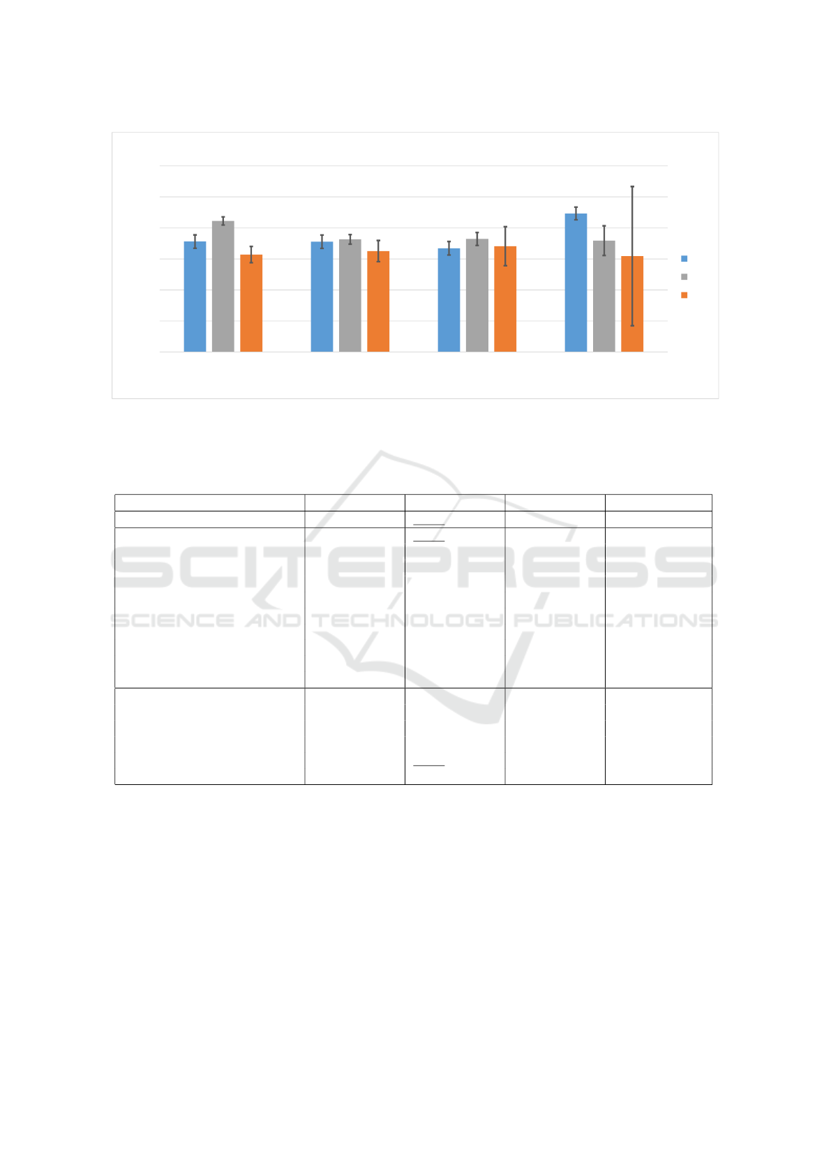
AUC Accuracy Precision Recall

Classification results (%)

Classification metrics

Comparison of testing single-trial classification performance

LDA

CNN

RNN

Figure 2: Classiﬁcation average results in the testing phase. It can be observed that LDA and CNN slightly outperformed

RNN in accuracy. RNNs were associated with unstable recall, as seen from its high standard deviation (black line).

Table 1: Average cross-validation classiﬁcation results based on the neural network parameter settings. Averages from 30

repetitions and related sample standard deviations (in brackets) are reported. The best performing models from each category

are highlighted in bold and subsequently used for testing.

Changed parameter AUC Accuracy Precision Recall

Baseline LDA (Va

reka, 2020) 61.77 % (0.9) 61.76 % (0.91) 61.45 % (1.9) 64.64 % (1.48)

Baseline CNN (Va

reka, 2020) 66.12 % (0.68) 62.18 % (0.94) 62.76 % (1.95) 61.34 % (2.63)

RELUs instead of ELUs 66.36 % (0.62) 61.85 % (1.15) 62.7 % (2.19) 60.1 % (3.04)

Filter size (3, 30) 65.84 % (0.49) 61.95 % (1.18) 62.7 % (2.1) 60.5 % (3.91)

12 conv. ﬁlters 66.31 % (0.51) 61.83 % (1.1) 62.3 % (2.21) 61.6 % (3.08)

No batch normalization 65.99 % (0.77) 60.55 % (1.52) 61.02 % (3.16) 61.5 % (7.21)

Dropout 0.2 67.67 % (0.65) 60.8 % (1.49) 61.33 % (2.31) 60.33 % (4.0)

No dropout 68.63 % (1.11) 59.49 % (1.2) 59.61 % (1.93) 60.7 % (4.44)

Dense (150) 66.07 % (0.8) 61.81 % (0.95) 62.33 % (1.83) 61.18 % (2.49)

Two dense l. (120-60) 65.72 % (0.77) 62.11 % (0.9) 63.14 % (2.03) 59.5 % (2.55)

Max- instead of AvgPool 64.23 % (1.15) 58.94 % (1.94) 60.22 % (4.18) 59.24 % (13.76)

Baseline RNN 65.68 % (0.85) 56.92 % (1.74) 57.61 % (2.31) 56.25 % (8.11)

LSTM(6) 65.79 % (1.04) 58.28 % (1.25) 58.33 % (2.48) 61.32 % (7)

LSTM(4) 65.41 % (1.04) 57.95 % (1.81) 58.67 % (2.56) 57 % (9.73)

LSTM(6), dropout 0.7 62.71 % (1.39) 58.99 % (1.47) 60.09 % (3.46) 58.35 % (11.02)

LSTM(6), dropout 0.8 60.63 % (1.32) 59.92 % (1.73) 61.49 % (3.81) 57.65 % (11.06)

LSTM(6), dropout 0.9 54.92 % (2.95) 56.89 % (4.86) 59.34 % (7.07) 55.8 % (25.3)

processing. No parameter decision was based on the

holdout set.

Table 1 shows results of cross-validation. The conﬁg-

uration with the highest accuracy was highlighted and

used for the testing phase. Figure 2 show the classiﬁ-

cation results.

5 DISCUSSION

As seen from the results, CNN yielded similar per-

formance to the baseline LDA. RNN accuracy was

slightly lower. Moreover, CNN results were far more

stable, as seen from the RNN high standard deviation

of recall.

The validation set experiments revealed that a

combination of the ELU activation, batch normaliza-

tion, dropout, and average pooling was preferable for

CNN (Va

reka, 2020). A substantial regularization

was necessary because of a large number of trainable

parameters for the RNN (120,592 for the LSTM(6)

network). In the cross-validation experiments, the

dropout of 0.8 yielded the highest classiﬁcation ac-

curacy.

Comparison of Convolutional and Recurrent Neural Networks for the P300 Detection

189

Similar single-trial P300 classiﬁcation perfor-

mance has been commonly reported in the litera-

ture. For example, in (Haghighatpanah et al., 2013),

65 % single-trial accuracy was achieved (using one to

three EEG channels and personalized training data).

In (Sharma, 2017), 40 % to 66 % classiﬁcation accu-

racy was reported, highly dependent on the individ-

ual tested. This paper presents comparable classiﬁca-

tion accuracy that was achieved using a multi-subject

dataset. Therefore, time-consuming training data col-

lection for each new user might be avoided, and long

training times of deep neural networks no longer pose

a problem. However, despite being successful, this

paper did not conﬁrm their beneﬁts over traditional

methods.

Even though LSTM did not outperform other clas-

siﬁers in the presented P300 experiments, it could be-

come valuable as a layer in a more complex model.

For example, in (Ditthapron et al., 2019), an LSTM

layer has been used in a multi-task autoencoder. First,

CNN layers were used to capture spatial domain fea-

tures, and LSTM was used for temporal relationship.

The resulting latent vector was either used to recon-

struct the input or for the P300 classiﬁcation. A simi-

lar approach could be applied in future work.

This study has several limitations. First, classiﬁ-

cation results on school-age children outside the labo-

ratory environment may not be generalized to a more

typical BCI population. Moreover, despite careful

manual tuning of hyperparameters, there might be an-

other RNN architecture outperforming the presented

CNN architecture that has not been discovered.

6 CONCLUSION

The presented experiments demonstrated that suc-

cessful P300 detection is possible for a multi-subject

dataset with all presented models (LDA, CNN, RNN).

However, when directly comparing CNN and RNN,

CNN appeared superior. It yielded comparable classi-

ﬁcation accuracy, more stable results, and was easier

to conﬁgure. The presented ofﬂine experiments can

be further reproduced in an online BCI. More exper-

iments into stacking CNN and RNN layers could be

the aim of future work.

ACKNOWLEDGEMENTS

This work was supported by the University speciﬁc

research project SGS-2019-018 Processing of hetero-

geneous data and its specialized applications. Special

thanks go to Master’s students Patrik Harag and Mar-

tin Matas for their initial experiments that inspired

this work.

REFERENCES

Blankertz, B., Lemm, S., Treder, M., Haufe, S., and Muller,

K. (2011). Single-trial analysis and classiﬁcation of

ERP components - a tutorial. NeuroImage, 56(2):814–

825.

Chollet, F. et al. (2015). Keras. https://keras.io.

Clevert, D.-A., Unterthiner, T., and Hochreiter, S. (2016).

Fast and accurate deep network learning by exponen-

tial linear units (ELUs). CoRR, abs/1511.07289.

Deng, L. and Yu, D. (2014). Deep learning: Methods

and applications. Foundations and Trends

 in Sig-

nal Processing, 7(3–4):197–387.

Ditthapron, A., Banluesombatkul, N., Ketrat, S., Chuang-

suwanich, E., and Wilaiprasitporn, T. (2019). Uni-

versal joint feature extraction for p300 eeg classiﬁ-

cation using multi-task autoencoder. IEEE Access,

7:68415–68428.

Farwell, L. A. and Donchin, E. (1988). Talking off the top of

your head: Toward a mental prosthesis utilizing event-

related brain potentials. Electroencephalography and

Clinical Neurophysiology, 70:510–523.

Haghighatpanah, N., Amirfattahi, R., Abootalebi, V., and

Nazari, B.(2013). A single channel-single trial P300

detection algorithm. In 2013 21st Iranian Conference

on Electrical Engineering (ICEE),pages 1–5.

Kingma, D. P. and Ba, J. (2014). Adam: A

method for stochastic optimization. cite

arxiv:1412.6980Comment: Published as a con-

ference paper at the 3rd International Conf. for

Learning Representations, San Diego, 2015.

Ledoit, O. and Wolf, M. (2004). Honey, i shrunk the sample

covariance matrix. The Journal of Portfolio Manage-

ment, 30(4):110–119.

Lotte, F., Bougrain, L., Cichocki, A., Clerc, M., Con-

gedo, M., Rakotomamonjy, A., and Yger, F. (2018).

A review of classiﬁcation algorithms for EEG-based

brain–computer interfaces: a 10 year update. Journal

of Neural Engineering, 15(3):031005.

Luck, S. J. (2005). An introduction to the event-related po-

tential technique. MIT Press, Cambridge, MA.

Manyakov, N. V., Chumerin, N., Combaz, A., and

Van Hulle, M. M. (2011). Comparison of classi-

ﬁcation methods for P300 brain-computer interface

on disabled subjects. Intell. Neuroscience, 2011:2:1–

2:12.

McFarland, D. J. and Wolpaw, J. R. (2011). Brain-computer

interfaces for communication and control. Commun.

ACM, 54(5):60–66.

Mou

cek, R., Va

reka, L., Prokop, T.,

ebet

ak, J., and Br

uha,

P. (2017). Event-related potential data from a guess

the number brain-computer interface experiment on

school children. Scientiﬁc Data, 4.

BIOSIGNALS 2021 - 14th International Conference on Bio-inspired Systems and Signal Processing

190

Mou

cek, R., Va

reka, L., Prokop, T.,

ebet

ak, J., and Br

uha,

P. (2019). Replication Data for: Evaluation of con-

volutional neural networks using a large multi-subject

P300 dataset.

Pinegger, A. and M

uller-Putz, G. (2017). No training, same

performance!? - a generic P300 classiﬁer approach. In

Proceedings of the 7th International BCI Conference

Graz 2017.

Polich, J. (2007). Updating p300: an integrative the-

ory of p3a and p3b. Clinical neurophysiology,

118(10):2128–2148.

Riggins, T. and Scott, L. S. (2020). P300 develop-

ment from infancy to adolescence. Psychophysiology,

57(7):e13346.

Roy, Y., Banville, H. J., Albuquerque, I., Gramfort, A., Falk,

T. H., and Faubert, J. (2019). Deep learning-based

electroencephalography analysis: a systematic review.

CoRR, abs/1901.05498.

Schirrmeister, R. T., Springenberg, J. T., Fiederer, L. D. J.,

Glasstetter, M., Eggensperger, K., Tangermann, M.,

Hutter, F., Burgard, W., and Ball, T. (2017). Deep

learning with convolutional neural networks for brain

mapping and decoding of movement-related informa-

tion from the human EEG. CoRR, abs/1703.05051.

Sharma, N. (2017). Single-trial P300 classiﬁcation using

PCA with lda, QDA and neural networks. CoRR,

abs/1712.01977.

Sikka, A., Jamalabadi, H., Krylova, M., Alizadeh, S.,

van der Meer, J. N., Danyeli, L., Deliano, M., Vicheva,

P., Hahn, T., Koenig, T., Bathula, D. R., and Wal-

ter, M. (2020). Investigating the temporal dynam-

ics of electroencephalogram (EEG) microstates using

recurrent neural networks. Human Brain Mapping,

41(9):2334–2346.

Tan, D. S. and Nijholt, A. (2010). Brain-Computer In-

terfaces: Applying Our Minds to Human-Computer

Interaction. Springer Publishing Company, Incorpo-

rated, 1st edition.

reka, L. (2020). Evaluation of convolutional neu-

ral networks using a large multi-subject P300

dataset. Biomedical Signal Processing and Control,

58:101837.

Vos, M. D., Kroesen, M., Emkes, R., and Debener, S.

(2014). P300 speller BCI with a mobile EEG sys-

tem: comparison to a traditional ampliﬁer. Journal of

Neural Engineering, 11(3):036008.

Comparison of Convolutional and Recurrent Neural Networks for the P300 Detection

191