
Video Camera Identification from Sensor Pattern Noise with a
Constrained ConvNet
Derrick Timmerman
1,∗ a
, Guru Swaroop Bennabhaktula
1,∗ b
, Enrique Alegre
2 c
and George Azzopardi
1 d
1
Bernoulli Institute for Mathematics, Computer Science and Artificial Intelligence,
University of Groningen, The Netherlands
2
Group for Vision and Intelligent Systems, Universidad de Le
´
on, Spain
Keywords:
Source Camera Identification, Video Device Identification, Video Forensics, Sensor Pattern Noise.
Abstract:
The identification of source cameras from videos, though it is a highly relevant forensic analysis topic, has
been studied much less than its counterpart that uses images. In this work we propose a method to identify
the source camera of a video based on camera specific noise patterns that we extract from video frames. For
the extraction of noise pattern features, we propose an extended version of a constrained convolutional layer
capable of processing color inputs. Our system is designed to classify individual video frames which are in
turn combined by a majority vote to identify the source camera. We evaluated this approach on the benchmark
VISION data set consisting of 1539 videos from 28 different cameras. To the best of our knowledge, this is the
first work that addresses the challenge of video camera identification on a device level. The experiments show
that our approach is very promising, achieving up to 93.1% accuracy while being robust to the WhatsApp and
YouTube compression techniques. This work is part of the EU-funded project 4NSEEK focused on forensics
against child sexual abuse.
1 INTRODUCTION
Source camera identification of digital media plays an
important role in counteracting problems that come
along with the simplified way of sharing digital con-
tent. Proposed solutions aim to reverse-engineer the
acquisition process of digital content to trace the ori-
gin, either on a model or device level. Whereas the
former aims to identify the brand and model of a cam-
era, the latter aims at identifying a specific instance of
a particular model. Detecting the source camera that
has been used to capture an image or record a video
can be crucial to point out the actual owner of the
content, but could also serve as additional evidence
in court.
Proposed techniques typically aim to identify the
source camera by extracting noise patterns from the
digital content. Noise patterns can be thought of as
a
https://orcid.org/0000-0002-9797-8261
b
https://orcid.org/0000-0002-8434-9271
c
https://orcid.org/0000-0003-2081-774X
d
https://orcid.org/0000-0001-6552-2596
∗
Derrick Timmerman and Guru Swaroop Bennabhak-
tula are both first authors.
an invisible trace, intrinsically generated by a partic-
ular device. These traces are the result of imperfec-
tions during the manufacturing process and are con-
sidered unique for an individual device (Luk
´
a
ˇ
s et al.,
2006). By its unique nature and its presence on every
acquired content, the noise pattern functions as an in-
strument to identify the camera model.
Within the field of source camera identification a
distinction is made between image and video camera
identification. Though a digital camera can capture
both images and videos, in a recent study it is experi-
mentally shown that a system designed to identify the
camera model of a given image cannot be directly ap-
plied to the problem of video camera model identifi-
cation (Hosler et al., 2019). Therefore, separate tech-
niques are required to address both problems.
Though great effort is put into identifying the
source camera of an image, significantly less research
has been conducted so far on a similar task using dig-
ital videos (Milani et al., 2012). Moreover, to the best
of our knowledge, only a single study addresses the
problem of video camera model identification by uti-
lizing deep learning techniques (Hosler et al., 2019).
Given the potential of such techniques in combination
Timmerman, D., Bennabhaktula, G., Alegre, E. and Azzopardi, G.
Video Camera Identification from Sensor Pattern Noise with a Constrained ConvNet.
DOI: 10.5220/0010246804170425
In Proceedings of the 10th International Conference on Pattern Recognition Applications and Methods (ICPRAM 2021), pages 417-425
ISBN: 978-989-758-486-2
Copyright
c
2021 by SCITEPRESS – Science and Technology Publications, Lda. All rights reserved
417
with the prominent role of digital videos in shared
digital media, the main goal of this work is to fur-
ther explore the possibilities of identifying the source
camera at device level of a given video by investigat-
ing a deep learning pipeline.
In this paper we present a methodology to identify
the source camera device of a video. We train a deep
learning system based on the constrained convolu-
tional neural network architecture proposed by Bayar
and Stamm (2018) for the extraction of noise patterns,
to classify individual video frames. Subsequently, we
identify the video camera device by applying the sim-
ple majority vote after aggregating frame classifica-
tions per video.
With respect to current state-of-the-art ap-
proaches, we advance with the following contribu-
tions: i) to the best of our knowledge, we are the
first to address video camera identification on a de-
vice level by including multiple instances of the same
brand and model; ii) we evaluate the robustness of the
proposed method with respect to common video com-
pression techniques for videos shared on the social
media platforms, such as WhatsApp and YouTube;
iii) we propose a multi-channel constrained convo-
lutional layer, and conduct experiments to show its
effectiveness in extracting better camera features by
suppressing the scene content.
The rest of the paper is organized as follows. We
start by presenting an overview of model-based tech-
niques in source camera identification, followed by
current state-of-the-art approaches in Section 2. In
Section 3 we describe the methodology for the extrac-
tion of noise pattern features for the classification of
frames and videos. Experimental results along with
the data set description are provided in Section 4. We
provide a discussion of certain aspects of the proposed
work in Section 5 and finally, we draw conclusions in
Section 6.
2 RELATED WORK
In the past decades, several approaches have been pro-
posed to address the problem of image camera model
identification (Bayram et al., 2005; Li, 2010; Bondi
et al., 2016; Bennabhaktula. et al., 2020). Those
methodologies aim to extract noise pattern features
from the input image or video that characterise the re-
spective camera model. These noise patterns or traces
are the result of imperfections during the manufac-
turing process and are thought to be unique for every
camera model (Luk
´
a
ˇ
s et al., 2006). More specifically,
during the acquisition process at shooting time, cam-
era models perform series of sophisticated operations
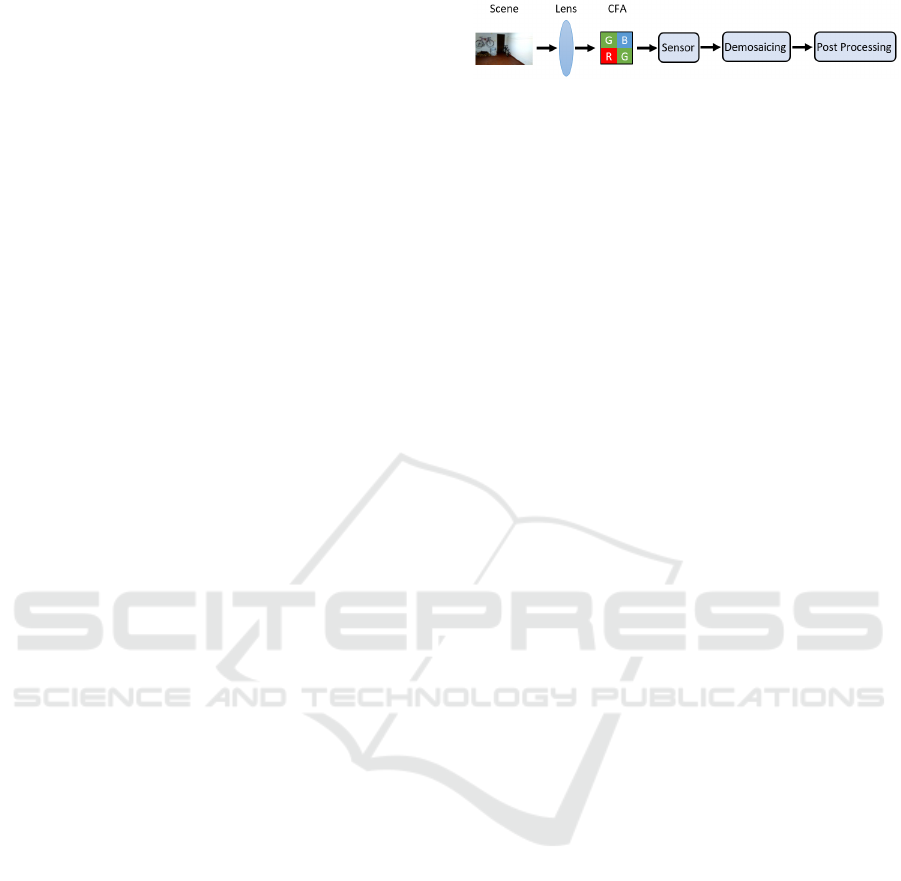
Figure 1: Acquisition pipeline of an image. Adapted from
Chen and Stamm (2015).
applied to the raw content before it is saved in mem-
ory, as shown in Fig. 1. During these operations, char-
acteristic traces are introduced to the acquired con-
tent, resulting in a unique noise pattern embedded in
the final output image or video. This noise pattern is
considered to be deterministic and irreversible for a
single camera sensor and is added to every image or
video the camera acquires (Caldell et al., 2010).
2.1 Model-based Techniques
Based on the hypothesis of unique noise patterns,
many image camera model identification algorithms
have been proposed aiming at capturing these char-
acteristic traces which can be divided into two main
categories: hardware and software based techniques.
Hardware techniques consider the physical compo-
nents of a camera such as the camera’s CCD (Charge
Coupled Device) sensor (Geradts et al., 2001) or the
lens (Dirik et al., 2008). Software techniques capture
traces left behind by internal components of the ac-
quisition pipeline of the camera, such as the sensor
pattern noise (SPN) (Lukas et al., 2006) or demosaic-
ing strategies (Milani et al., 2014).
2.2 Data-driven Technologies
Although model-based techniques have shown to
achieve good results, they all rely on manually de-
fined procedures to extract (parts of) the characteris-
tic noise patterns. Better results are achieved by ap-
plying deep learning techniques, also known as data-
driven methodologies. There are a few reasons why
these methods work so well. First, these techniques
are easily scalable since they learn directly from data.
Therefore, adding new camera models does not re-
quire manual effort and is a straightforward process.
Second, these techniques often perform better when
trained with large amounts of data, allowing us to
take advantage of the abundance of digital images and
videos publicly available on the internet.
Given their ability to learn salient features directly
from data, convolutional neural networks (ConvNets)
are frequently incorporated to address the problem of
image camera model identification. To further im-
prove the feature learning process of ConvNets, tools
from steganalysis have been adapted that suppress the
high level scene content of an image (Qiu et al., 2014).
ICPRAM 2021 - 10th International Conference on Pattern Recognition Applications and Methods
418
In their existing form, convolutional layers tend to ex-
tract features that capture the scene content of an im-
age as opposed to the desired characteristic camera
detection features, i.e. the noise patterns. This behav-
ior was first observed by Chen et al. (2015) in their
study to detect traces of median filtering. Since the
ConvNet was not able to learn median filtering detec-
tion features by feeding images directly to the input
layer, they extracted the median filter residual (i.e. a
high dimensional feature set) from the image and pro-
vided it to the ConvNet’s input layer, resulting in an
improvement in classification accuracy.
Following the observations of Chen et al. (2015),
two options for the ConvNet have emerged that sup-
press the scene content of an image: using a prede-
termined high-pass filter (HPF) within the input layer
(Pibre et al., 2016) or the adaptive constrained convo-
lutional layer (Bayar and Stamm, 2016). Whereas the
former requires human intervention to set the prede-
termined filter, the latter is able to jointly suppress the
scene content and to adaptively learn relationships be-
tween neighbouring pixels. Initially designed for im-
age manipulation detection, the constrained convolu-
tional layer shows to achieve state-of-the-art results in
other digital forensic problems as well, including im-
age camera model identification (Bayar and Stamm,
2017).
Although deep learning techniques are commonly
used to identify the source camera of an image, it
was not until very recently that these techniques were
applied to video camera identification. Therefore,
the work of Hosler et al. (2019) is one of the few
ones closely related to the ideas we propose. Hosler
et al. adopted the constrained ConvNet architecture
proposed by Bayar and Stamm (2018), although they
removed the constrained convolutional layer due to
its incompatibility with color inputs. To identify the
camera model of a video, in their work they train the
ConvNet to produce classification scores for patches
extracted from video frames. Subsequently, individ-
ual patch scores are combined to produce video-level
classifications, as single-patch classifications showed
to be insufficiently reliable.
The ideas we propose in this work differ from
Hosler et al. (2019) in the following ways. Instead
of removing the constrained convolutional layer, we
propose an extended version of it by making it suit-
able for color inputs. Furthermore, instead of using
purely different camera models, we include 28 cam-
era devices among which 13 are of the same brand
and model, allowing us to investigate the problem in a
device-based manner. Lastly, we provide the network
with the entire video frame to extract noise pattern
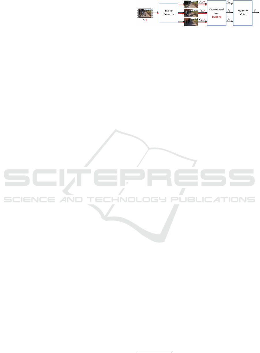
Figure 2: High level overview of our methodology. Dur-
ing the training process, highlighted in red, N frames are
extracted from a video V , inheriting the same label y to
train the ConstrainedNet. During evaluation, highlighted in
black, the ConstrainedNet produces ˆy
n
labels for N frames
to predict the label ˆy of the given video.
features, whereas Hosler et al. use smaller patches
extracted from frames.
3 METHODOLOGY
In Fig. 2 we illustrate a high level overview of our
methodology, which mainly consists of the following
steps: i) extraction of frames from the input video; ii)
classification of frames by the trained Constrained-
Net, and iii) aggregation of frame classifications to
produce video-level classifications.
In the following sections, the frame extraction
process is explained, as well as the voting procedure.
Furthermore, architectural details of the Constrained-
Net are provided.
3.1 ConstrainedNet
We propose a ConstrainedNet which we make pub-
licly available
1
, that we train with deep learning for
video device identification based on recent techniques
in image (Bayar and Stamm, 2018) and video (Hosler
et al., 2019) camera identification. We adapt the con-
strained ConvNet architecture proposed by Bayar and
Stamm (2018) and apply a few modifications. Given
the strong variation in video resolutions within the
data set that we use, we set the input size of our net-
work equals to the smallest video resolution of 480 ×
800 pixels. Furthermore, we increase the size of the
first two fully-connected layers from 200 to 1024, and
most importantly, we extend the original constrained
convolutional layer by adapting it for color inputs.
The constrained convolutional layer was origi-
nally proposed by Bayar and Stamm (2016) and is a
modified version of a regular convolutional layer. The
idea behind this layer is that relationships exist be-
tween neighbouring pixels independent of the scene
content. Those relationships are characteristic of a
camera device and are estimated by jointly suppress-
ing the high-level scene content and learning connec-
tions between a pixel and its neighbours, also referred
1
https://github.com/zhemann/vcmi
Video Camera Identification from Sensor Pattern Noise with a Constrained ConvNet
419

to as pixel value prediction errors (Bayar and Stamm,
2016). Suppressing the high-level scene content is
necessary to prevent the learning of scene-related fea-
tures. Therefore, the filters of the constrained con-
volutional layer are restricted to only learn a set of
prediction error filters, and are not allowed to evolve
freely. Prediction error filters operate as follows:
1. Predict the center pixel value of the filter support
by the surrounding pixel values.
2. Subtract the true center pixel value from the pre-
dicted value to generate the prediction error.
More formally, Bayar and Stamm placed the follow-
ing constraints on K filters w
(1)
k
in the constrained
convolutional layer:
(
w
(1)
k
(0,0) = −1
∑
m,n6=0
w
(1)
k
(m,n) = 1
(1)
where the superscript
(1)
denotes the first layer of
the network, w
(1)
k
(m,n) is the filter weight at posi-
tion (m,n) and w
(1)
k
(0,0) the filter weight at the cen-
ter position of the filter support. The constraints are
enforced during the training process after the filter’s
weights are updated in the backpropagation step. The
center weight value of each filter kernel is then set to
−1 and the remaining weights are normalized such
that their sum equals 1.
3.1.1 Extended Constrained Layer
The originally proposed constrained convolutional
layer only supports gray-scale inputs. We propose an
extended version of this layer by allowing it to process
inputs with three color channels. Considering a con-
volutional layer, the main difference between gray-
scale and color inputs is the number of kernels within
each filter. Whereas gray-scale inputs require one ker-
nel, color inputs require three kernels. Therefore, we
modify the constrained convolutional layer by simply
enforcing the constraints in Eq. 1 to all kernels of each
filter. The constraints enforced on K 3-dimensional
filters in the constrained convolutional layer can be
formulated as follows:
w
(1)
k
j
(0,0) = −1
∑
m,n6=0
w
(1)
k
j
(m,n) = 1
(2)
where j ∈ {1,2,3}. Moreover, w
(1)
k
j
denotes the j
th
kernel of the k
th
filter in the first layer of the ConvNet.
3.2 Frame Extraction
While other studies extract the first N frames of each
video (Shullani et al., 2017), we extract a given num-
ber of frames equally spaced in time across the en-
tire video. For example, to extract 200 frames from
a video consisting of 1000 frames, we would extract
frames [5, 10, .., 1000] whereas for a video of 600
frames we would extract frames [3, 6, .., 600]. Fur-
thermore, we did not impose requirements on a frame
to be selected, in contrast to Hosler et al. (2019).
3.3 Voting Procedure
The camera device of a video under investigation is
identified as follows. We first create the set I consist-
ing of K frames extracted from video v, as explained
in Section 3.2. Then, every input I
k
is processed by
the (trained) ConstrainedNet, resulting in the proba-
bility vector z
k
. Each value in z
k
represents a camera
device c ∈ C where C is the set of camera devices un-
der investigation. We determine the predicted label ˆy
k
for input I
k
by selecting label y
c
of the camera device
that achieves the highest probability. Eventually, we
obtain the predicted camera device label ˆy
v
for video
v by majority voting on ˆy
k
where k ∈ [1,K].
4 EXPERIMENTS AND RESULTS
4.1 Data Set
We used the publicly available VISION data set
(Shullani et al., 2017). It was introduced to provide
digital forensic experts a realistic set of digital im-
ages and videos captured by modern portable camera
devices. The data set includes a total of 35 camera de-
vices representing 11 brands. Moreover, the data set
consists of 6 camera models with multiple instances
(13 camera devices in total), suiting our aim to inves-
tigate video camera identification at device level.
The VISION data set consists of 1914 videos in
total which can be subdivided into native versions and
their corresponding social media counterparts. The
latter are generated by exchanging native videos via
social media platforms. There are 648 native videos,
622 are shared through YouTube and 644 via What-
sApp. While both YouTube and WhatsApp apply
compression techniques to the input video, YouTube
maintains the original resolution while WhatsApp re-
duces the resolution to a size of 480 × 848 pixels.
Furthermore, the videos represent three different sce-
narios: flat, indoor, and outdoor. The flat scenario
contains videos depicting flat objects such as walls or
ICPRAM 2021 - 10th International Conference on Pattern Recognition Applications and Methods
420
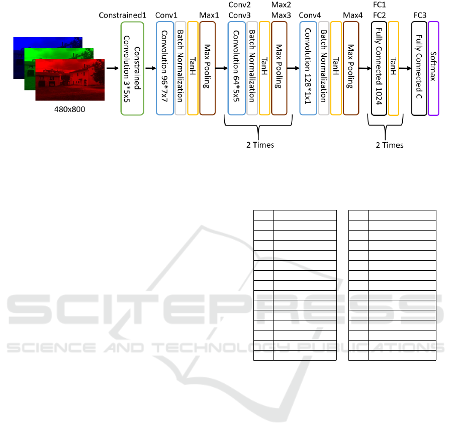
Figure 3: Architecture of the proposed ConstrainedNet.
blue skies, and are often largely similar across mul-
tiple camera devices. The indoor scenario comprises
videos depicting indoor settings, such as stores and
offices, whereas the latter scenario contains videos
showing outdoor areas including gardens and streets.
Each camera device consists of at least two native
videos for every scenario.
4.1.1 Camera Device Selection Procedure
Rather than including each camera device of the VI-
SION data set, we selected a subset of camera devices
that excludes devices with very few videos. We deter-
mined the appropriate camera devices based on the
number of available videos and the camera device’s
model. More explicitly, we included camera devices
that met either of the following criteria:
1. The camera device contains at least 18 native
videos, which are also shared through both
YouTube and Whatsapp.
2. More than one instance of the camera device’s
brand and model occur in the VISION data set.
We applied the first criterion to exclude camera de-
vices that contained very few videos. Exceptions are
made for devices of the same brand and model, as in-
dicated by the second criterion. Those camera devices
are necessary to exploit video device identification.
Furthermore, we excluded the Asus Zenfone 2 Laser
camera model as suggested by Shullani et al. (2017),
resulting in a subset of 28 camera devices out of 35,
shown in Table 1. The total number of videos sum up
to 1539 of which 513 are native and 1026 are social
media versions. In Fig. 4 an overview of the video
duration for the 28 camera devices is provided.
Table 1: The set of 28 camera devices we used to conduct
the experiments, of which 13 are of the same brand and
model, indicated by the superscript.
ID Device ID Device
1 iPhone 4 15 Huawei P9
2 iPhone 4s* 16 Huawei P9 Lite
3 iPhone 4s* 17 Lenovo P70A
4 iPhone 5** 18 LG D290
5 iPhone 5** 19 OnePlus 3
§
6 iPhone 5c
†
20 OnePlus 3
§
7 iPhone 5c
†
21 Galaxy S3 Mini
k
8 iPhone 5c
†
22 Galaxy S3 Mini
k
9 iPhone 6
††
23 Galaxy S3
10 iPhone 6
††
24 Galaxy S4 Mini
11 iPhone 6 Plus 25 Galaxy S5
12 Huawei Ascend 26 Galaxy Tab 3
13 Huawei Honor 5C 27 Xperia Z1 Compact
14 Huawei P8 28 Redmi Note 3
4.2 Frame-based Device Identification
We created balanced training and test sets in the fol-
lowing way. We first determined the lowest number
of native videos among the 28 camera devices that we
included based on the camera device selection proce-
dure. We used this number to create balanced training
and test sets of native videos in a randomized way,
maintaining a training-test split of 55%/45%. More-
over, we ensured that per camera device, each sce-
nario (flat, indoor, and outdoor) is represented in both
the training and test set. Concerning this experiment,
the lowest number of native videos was 13 through
which we randomly picked 7 and 6 native videos per
camera device for the training and test sets, respec-
tively. Subsequently, we added the WhatsApp and
YouTube versions for each native video, tripling the
size of the data sets. This approach ensured that a na-
tive video and its social media versions always belong
to either the training set or test set, but not both. Al-
though the three versions of a video differ in quality
and resolution, they still depict the same scene con-
Video Camera Identification from Sensor Pattern Noise with a Constrained ConvNet
421

Figure 4: Boxplot showing the means and quartiles of the
video durations in seconds for the 28 camera devices. Out-
liers are not shown in this plot.
tent which could possibly lead to biased results if they
were distributed over both the training set and test set.
Eventually, this led to 21 training videos (7 native,
7 WhatsApp, and 7 YouTube) and 18 test videos (6
native, 6 WhatsApp, and 6 YouTube) being included
per camera device, resulting in a total number of 588
training and 504 test videos. Due to the limited num-
ber of available videos per camera device, we did not
have the luxury to create a validation set. We ex-
tracted 200 frames from every video following the
procedure as described in Section 3.2, resulting in a
total number of 117,600 training frames and 100,800
test frames. Each training frame inherited the same
label as the camera device that was used to record the
video.
Furthermore, we performed this experiment in
two different settings to investigate the performance
of our extended constrained convolutional layer. In
the first setting we used the ConstrainedNet as ex-
plained in Section 3.1, whereas we removed the con-
strained convolutional layer in the second setting. We
refer to the network in the second setting as the Un-
constrainedNet.
We trained both the ConstrainedNet and the Un-
constrainedNet for 30 epochs in batches of 128
frames. We used the stochastic gradient descent
(SGD) during the backpropagation step to minimize
the categorical cross-entropy loss function. To speed
up the training time and convergence of the model,
we used the momentum and decay strategy. The mo-
mentum was set to 0.95 and we used a learning rate
of 0.001 with step rate decay of 0.0005 after every
training batch. The training took roughly 10 hours to
complete for each of both architectures
2
.
We measured the performance of the Constrained-
Net and the UnconstrainedNet by calculating the
video classification accuracy on the test set. After ev-
ery training epoch we saved the network’s state and
2
We used the deep learning library Keras on top of Ten-
sorflow to create, train, and evaluate the ConstrainedNet and
UnconstrainedNet. Training was performed using a Nvidia
Tesla V100 GPU.
calculated the video classification accuracy as fol-
lows:
1. Classify each frame in the test set.
2. Aggregate frame classifications per video.
3. Classify the video according to the majority vote
as described in Section 3.3.
4. Divide the number of correctly classified test
videos by the total number of test videos.
In addition to the test accuracy, we also calcu-
lated the video classification accuracy for the different
scenarios (flat, indoor, outdoor) and versions (native,
WhatsApp, YouTube). The different scenarios are
used to exploit the extraction of noise pattern features
and to determine the influence of high-level scene
content. The different video versions are used to in-
vestigate the impact of different compression tech-
niques.
4.2.1 Results
In Fig. 5 we show the progress of the test accuracy for
the ConstrainedNet and the UnconstrainedNet. It can
be observed that the performance significantly im-
proved by the introduction of the constrained convo-
lutional layer. The ConstrainedNet achieved its peak-
performance after epoch 25 with an overall accuracy
of 66.5%. Considering the accuracy per scenario,
we observed 89.1% accuracy for flat scenario videos,
53.7% for indoor scenarios, and 55.2% accuracy for
the outdoor. Results for the individual scenarios are
shown in Fig. 6.
Since the flat scenario videos achieved a signifi-
cantly higher classification accuracy compared to the
others, we limited ourselves to this scenario dur-
ing the investigation of how different compression
techniques would affect the results. In Fig. 7 we
show the confusion matrices that the ConstrainedNet
achieved from the perspective of different compres-
sion techniques (i.e. native, WhatsApp and YouTube).
We achieved 89.7% accuracy on the native versions,
93.1% on the WhatsApp versions, and 84.5% on the
YouTube ones.
5 DISCUSSION
From the results in Fig. 5 it can be observed that
the constrained convolutional layer significantly con-
tributes to the performance of our network. This sug-
gests this layer is worth further investigating its po-
tential in light of digital forensic problems on color
inputs. Furthermore, in Fig. 6 it is shown that the clas-
sification accuracy greatly differs between the three
ICPRAM 2021 - 10th International Conference on Pattern Recognition Applications and Methods
422
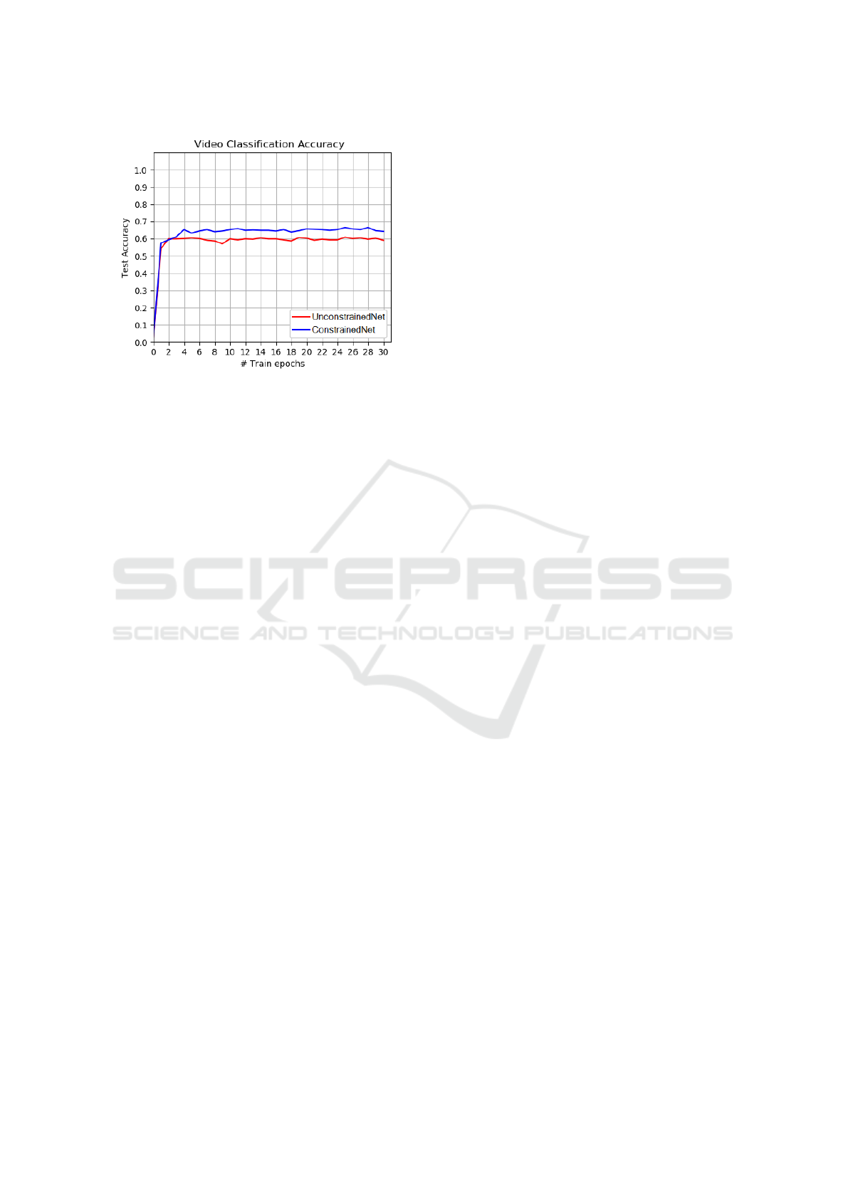
Figure 5: Progress of the test video classification accuracy
for the ConstrainedNet and UnconstrainedNet.
scenarios; flat, indoor, and outdoor. Whereas the
indoor and outdoor scenarios achieve accuracies of
53.7% and 55.2%, respectively, we observe an ac-
curacy of 89.1% for the flat scenario videos. Given
the high degree of similarity between flat scenario
videos from multiple camera devices, the results sug-
gest that the ConstrainedNet has actually extracted
characteristic noise pattern features for the identifi-
cation of source camera devices. The results also
indicate that indoor and outdoor scenario videos are
less suitable to extract noise pattern features for de-
vice identification. This difference could lie in the
absence or lack of video homogeneity. Compared to
the flat scenario videos, indoor and outdoor scenario
videos typically depict a constantly changing scene.
As a consequence, the dominant features of a video
frame are primarily scene-dependent, making it sig-
nificantly harder for the ConstrainedNet to extract the
scene-independent features, that is, the noise pattern
features.
Fig. 7 shows that our methodology is robust
against the compression techniques applied by What-
sApp and YouTube. While we observe an accuracy of
89.7% for the native versions of flat scenario videos,
we observe accuracies of 93.1% and 84.5% for the
WhatsApp and YouTube versions, respectively. The
high performance of WhatsApp versions could be
due to the similarity in size (i.e. resolution) between
WhatsApp videos and our network’s input layer. As
explained in Section 4.1, the WhatsApp compression
techniques resize the resolution of a video to the size
of 480 × 848 pixels, becoming nearly identical to the
network’s input size of 480 × 800 pixels. This is in
contrast to the techniques applied by YouTube, which
respect the original resolution.
These results indicate that the content homogene-
ity of a video frame plays an important role in the
classification process of videos. Therefore, we sug-
gest to search for homogeneous patches within each
video frame, and only use those patches for the clas-
sification of a video. This would limit the influence
of scene-related features, forcing the network to learn
camera device specific features.
By proposing this methodology we aim to support
digital forensic experts in order to identify the source
camera device of digital videos. We have shown that
our approach is able to identify the camera device of a
video with an accuracy of 89.1%. This accuracy fur-
ther improves to 93.1% when considering the What-
sApp versions. Although the experiments were per-
formed on known devices, we believe this work could
be extended by matching pairs of videos of known and
unknown devices too. In that case, the Constrained-
Net may be adopted in a two-part deep learning so-
lution where it would function as the feature extrac-
tor, followed by a similarity network (e.g. Siamese
Networks) to determine whether two videos are ac-
quired by the same camera device. To the best of
our knowledge, this is the first work that addresses the
task of device-based video identification by applying
deep learning techniques.
In order to further improve the performance of
our methodology, we believe it is worth investigat-
ing the potential of patch-based approaches wherein
the focus lies on the homogeneity of a video. More
specifically, only homogeneous patches would be ex-
tracted from frames and used for the classification
of a video. This should allow the network to bet-
ter learn camera device specific features, leading to
an improved device identification rate. Moreover, by
using patches the characteristic noise patterns remain
unaltered since they do not undergo any resize oper-
ation. In addition, this could significantly reduce the
complexity of the network, requiring less computa-
tional effort. Another aspect to investigate would be
the type of voting procedure. Currently, each frame
always votes for a single camera device even when
the ConstrainedNet is highly uncertain about which
device the frame is acquired by. To counteract this
problem, voting procedures could be tested that take
this uncertainty into account. For example, we could
require a certain probability threshold to vote for a
particular device. Another example would be to select
the camera device based on the highest probability af-
ter averaging the output probability vectors of frames
aggregated per video.
Video Camera Identification from Sensor Pattern Noise with a Constrained ConvNet
423
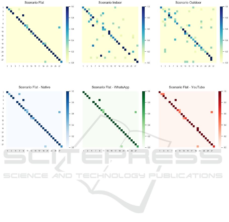
Figure 6: Confusion matrices for 28 camera devices showing the normalized classification accuracies achieved for the scenar-
ios flat, indoor, and outdoor.
Figure 7: Confusion matrices for 28 camera devices showing the normalized classification accuracies achieved on flat scenario
videos from the perspective of the native videos and their social media versions.
6 CONCLUSION
Based on the results that we achieved so far, we draw
the following conclusions. The extended constrained
convolutional layer contributes to increase in perfor-
mance. Considering the different types of videos, the
proposed method is more effective for videos with
flat (i.e. homogeneous) content, achieving an accu-
racy of 89.1%. In addition, the method shows to be
robust against the WhatsApp and YouTube compres-
sion techniques with accuracy rates up to 93.1% and
84.5%, respectively.
ACKNOWLEDGEMENTS
We thank the Center for Information Technology of
the University of Groningen for their support and for
providing access to the Peregrine high performance
computing cluster. This research has been funded
with support from the European Commission under
the 4NSEEK project with Grant Agreement 821966.
This publication reflects the views only of the authors,
and the European Commission cannot be held respon-
sible for any use which may be made of the informa-
tion contained therein.
REFERENCES
Bayar, B. and Stamm, M. C. (2016). A deep learning ap-
proach to universal image manipulation detection us-
ing a new convolutional layer. In Proceedings of the
4th ACM Workshop on Information Hiding and Multi-
media Security, pages 5–10.
Bayar, B. and Stamm, M. C. (2017). Design principles of
convolutional neural networks for multimedia foren-
sics. Electronic Imaging, 2017(7):77–86.
Bayar, B. and Stamm, M. C. (2018). Constrained convo-
lutional neural networks: A new approach towards
general purpose image manipulation detection. IEEE
Transactions on Information Forensics and Security,
13(11):2691–2706.
Bayram, S., Sencar, H., Memon, N., and Avcibas, I. (2005).
Source camera identification based on cfa interpola-
tion. In IEEE International Conference on Image Pro-
cessing 2005, volume 3, pages III–69. IEEE.
Bennabhaktula., G. S., Alegre., E., Karastoyanova., D., and
ICPRAM 2021 - 10th International Conference on Pattern Recognition Applications and Methods
424

Azzopardi., G. (2020). Device-based image matching
with similarity learning by convolutional neural net-
works that exploit the underlying camera sensor pat-
tern noise. In Proceedings of the 9th International
Conference on Pattern Recognition Applications and
Methods - Volume 1: ICPRAM,, pages 578–584. IN-
STICC, SciTePress.
Bondi, L., Baroffio, L., G
¨
uera, D., Bestagini, P., Delp,
E. J., and Tubaro, S. (2016). First steps toward cam-
era model identification with convolutional neural net-
works. IEEE Signal Processing Letters, 24(3):259–
263.
Caldell, R., Amerini, I., Picchioni, F., De Rosa, A., and
Uccheddu, F. (2010). Multimedia forensic techniques
for acquisition device identification and digital image
authentication. In Handbook of Research on Compu-
tational Forensics, Digital Crime, and Investigation:
Methods and Solutions, pages 130–154. IGI Global.
Chen, C. and Stamm, M. C. (2015). Camera model identi-
fication framework using an ensemble of demosaicing
features. In 2015 IEEE International Workshop on In-
formation Forensics and Security (WIFS), pages 1–6.
IEEE.
Chen, J., Kang, X., Liu, Y., and Wang, Z. J. (2015). Median
filtering forensics based on convolutional neural net-
works. IEEE Signal Processing Letters, 22(11):1849–
1853.
Dirik, A. E., Sencar, H. T., and Memon, N. (2008). Digital
single lens reflex camera identification from traces of
sensor dust. IEEE Transactions on Information Foren-
sics and Security, 3(3):539–552.
Geradts, Z. J., Bijhold, J., Kieft, M., Kurosawa, K., Kuroki,
K., and Saitoh, N. (2001). Methods for identification
of images acquired with digital cameras. In Enabling
technologies for law enforcement and security, vol-
ume 4232, pages 505–512. International Society for
Optics and Photonics.
Hosler, B., Mayer, O., Bayar, B., Zhao, X., Chen, C., Shack-
leford, J. A., and Stamm, M. C. (2019). A video cam-
era model identification system using deep learning
and fusion. In ICASSP 2019-2019 IEEE International
Conference on Acoustics, Speech and Signal Process-
ing (ICASSP), pages 8271–8275. IEEE.
Li, C.-T. (2010). Source camera identification using en-
hanced sensor pattern noise. IEEE Transactions on
Information Forensics and Security, 5(2):280–287.
Luk
´
a
ˇ
s, J., Fridrich, J., and Goljan, M. (2006). Detecting
digital image forgeries using sensor pattern noise. In
Security, Steganography, and Watermarking of Multi-
media Contents VIII, volume 6072, page 60720Y. In-
ternational Society for Optics and Photonics.
Lukas, J., Fridrich, J., and Goljan, M. (2006). Digital cam-
era identification from sensor pattern noise. IEEE
Transactions on Information Forensics and Security,
1(2):205–214.
Milani, S., Bestagini, P., Tagliasacchi, M., and Tubaro,
S. (2014). Demosaicing strategy identification via
eigenalgorithms. In 2014 IEEE International Con-
ference on Acoustics, Speech and Signal Processing
(ICASSP), pages 2659–2663. IEEE.
Milani, S., Fontani, M., Bestagini, P., Barni, M., Piva, A.,
Tagliasacchi, M., and Tubaro, S. (2012). An overview
on video forensics. APSIPA Transactions on Signal
and Information Processing, 1.
Pibre, L., Pasquet, J., Ienco, D., and Chaumont, M. (2016).
Deep learning is a good steganalysis tool when em-
bedding key is reused for different images, even if
there is a cover sourcemismatch. Electronic Imaging,
2016(8):1–11.
Qiu, X., Li, H., Luo, W., and Huang, J. (2014). A universal
image forensic strategy based on steganalytic model.
In Proceedings of the 2nd ACM workshop on Informa-
tion hiding and multimedia security, pages 165–170.
Shullani, D., Fontani, M., Iuliani, M., Al Shaya, O., and
Piva, A. (2017). Vision: a video and image dataset for
source identification. EURASIP Journal on Informa-
tion Security, 2017(1):15.
Video Camera Identification from Sensor Pattern Noise with a Constrained ConvNet
425
