Can We Detect Harmony in Artistic Compositions?

A Machine Learning Approach

Adam Vandor

, Marie Van Vollenhoven

, Gerhard Weiss

and Gerasimos Spanakis

1 a

Department of Data Science and Knowledge Engineering, Maastricht University, Maastricht, The Netherlands

Inﬁnity Games, Maastricht, The Netherlands

Keywords:

Artistic Compositions, Feature Extraction, Machine Learning.

Abstract:

Harmony in visual compositions is a concept that cannot be deﬁned or easily expressed mathematically, even

by humans. The goal of the research described in this paper was to ﬁnd a numerical representation of artistic

compositions with different levels of harmony. We ask humans to rate a collection of grayscale images based

on the harmony they convey. To represent the images, a set of special features were designed and extracted.

By doing so, it became possible to assign objective measures to subjectively judged compositions. Given

the ratings and the extracted features, we utilized machine learning algorithms to evaluate the efﬁciency of

such representations in a harmony classiﬁcation problem. The best performing model (SVM) achieved 80%

accuracy in distinguishing between harmonic and disharmonic images, which reinforces the assumption that

concept of harmony can be expressed in a mathematical way that can be assessed by humans.

1 INTRODUCTION

Harmony is an abstract concept that does not have

a formally precise deﬁnition. Depending on the do-

main, such as painting, music or architecture, har-

mony means something different to different persons.

When we think of harmony, we associate it with a

compilation of independent elements, which as a re-

sult create a consistent, pleasing arrangement. Even

though there exist well-known patterns that carry har-

monious sentiments in the eyes of the people, like

the golden-ratio (Di Dio et al., 2007) in images, the

inherent source of their harmonic nature is not obvi-

ous. The research described here aimed at exploring

whether the individual perception of harmony in im-

ages can be expressed in mathematical terms. Specif-

ically, our research aims at addressing the question

whether it is possible to use machine learning tech-

niques to generate a mathematically founded model

of a person’s subjective understanding of harmony.

Our hypothesis is that if machine learning mod-

els are able to be trained in order to conﬁdently pre-

dict the labels one would assign to the compositions,

then it would mean that there exists some numerical

representation of a composition that reﬂects its har-

monic level. Therefore, we need to extract features

https://orcid.org/0000-0002-0799-0241

from the compositions that can further be used by ma-

chine learning algorithms. The main difﬁculty of this

approach lies in the designing of such features that

carry general and meaningful information about the

compositions. We also need to take into considera-

tion that no classical data augmentation techniques -

such as rotation, translation, ﬂipping, etc. - can be

applied in the research, as the resulting images would

be completely new data points that might be assessed

differently.

After presenting a short overview of the state-of-

the-art techniques in Section 2, Section 3 outlines the

dataset and the process of feature extraction used in

our research, and describes the necessary transforma-

tions of the data and how the uncertain nature of the

target variables was handled, followed by the machine

learning framework used, and Section 4 shows the

experimental results achieved through machine learn-

ing.

2 RELATED WORK

On the technical side, visual feature extraction and

image classiﬁcation are broadly investigated topics

in the ﬁeld of Artiﬁcial Intelligence and Computer

Vision. Research and applications regarding object

Vandor, A., Van Vollenhoven, M., Weiss, G. and Spanakis, G.

Can We Detect Harmony in Artistic Compositions? A Machine Learning Approach.

DOI: 10.5220/0010244901870195

In Proceedings of the 13th International Conference on Agents and Artiﬁcial Intelligence (ICAART 2021) - Volume 2, pages 187-195

ISBN: 978-989-758-484-8

187

recognition cover several domains. In (Wu et al.,

2007) methods for leaf recognition are examined. In

(LeCun et al., 1990) the classiﬁcation of handwritten

digits is explored using back-propagation. There are a

number of other use cases, which consider computer

vision based approaches in order to analyze and iden-

tify meaningful patterns. In (Zhao et al., 1998) tech-

niques for face recognition are presented, in (Bharati

et al., 2004) the analysis of surface textures are in-

vestigated in order to assess the quality of produced

goods, and in (Deepa and Devi, 2011) a collection of

Artiﬁcial Intelligence based approached are surveyed

for medical image classiﬁcation.

Feature extraction methods play indispensable

roles in efﬁcient image classiﬁcation. Feature ex-

traction algorithms such as SIFT (Lowe, 1999) and

SURF (Bay et al., 2006) introduce techniques to ﬁnd

generally meaningful patterns in images. (Nixon and

Aguado, 2012) covers a broad range of feature extrac-

tion and image processing techniques, and (ping Tian

et al., 2013) reviews feature extraction and represen-

tation techniques for further image classiﬁcation.

On the philosophical side, the question that lies is

whether an abstract concept like harmony can be ex-

pressed by quantitative measures. On the one hand,

one argument, originating from Plato (Pappas, 2008)

is that concepts like beauty can be associated with

harmony, symmetry and unity. On the other hand,

research suggests that there are also emotional pro-

cesses that contribute to assessing aesthetics (Leder

et al., 2004).

When it comes to evaluating artistic creations of

computer programs, researchers have attempted to

measure the aesthetic value using a ratio of the per-

ceived order over complexity (Davis, 1936). How-

ever, most of the work focuses on describing concepts

like computational creativity and how it can be as-

sessed (Jordanous, 2012) but only a few approaches

exist that try to quantify the concept of harmony in

compositions, e.g. in (Salleh and Phon-Amnuaisuk,

2015) authors are assessing the aesthetic quality of

trochoids.

In this paper, a set of speciﬁc features is intro-

duced, which is directly applicable to the problem

of capturing the concept of harmony by carrying in-

formation about the arrangement of artistic composi-

tions. Our expectation is that if a machine learning

model can be trained to identify whether a composi-

tion is harmonic or not, then that would be a ﬁrst step

to build such a measure for quantifying such an ab-

stract concept.

3 METHODOLOGY

3.1 Dataset Collection

The dataset used in this research consists of a num-

ber of randomly generated visual compositions by the

application ’The Composition Game’

. Each com-

position displays a set of black and white shapes on

a square gray background. The position and rotation

of each shape are randomly generated. The size of

each shape is randomly drawn from a preset contin-

uous range. The amount of black and white shapes,

and the amount of circles, rectangles and triangles are

set prior to the image generation. Figure 1 shows a

few examples.

The participants’ task was to evaluate each com-

position and to assign a number to it from a discrete

range from 1 to 5, which they thought expresses the

level of harmony of the image the most, where 5

means very harmonic and 1 means very disharmonic.

We asked one participant to rate 8909 different com-

positions and we refer to this collection of composi-

tions and ratings as the dataset. In the future, we plan

to include data from more participants as the study is

ongoing.

3.2 Feature Extraction

In order to represent each composition as a vector in

an n-dimensional space, we need to assign n numer-

ical values to it. The resulting feature vector is the

concatenation of the extracted values and each com-

ponent of the vector corresponds to a feature.

One of the issues that arises is that some ex-

tracted features are highly dependent on the number

of shapes, which could result in feature vectors hav-

ing different lengths. For example, if a feature to be

used is given by the distances between each shape in

an image and the center of the image, then this feature

would consist of three values in case there are three

shapes in the image wheras it would consist of four

values in case the image contains four shapes. For this

reason, we use statistical properties (minimum, max-

imum, mean and standard deviation) of such features

rather than the individual values themselves. In this

way, the actual information related to such a feature is

not represented in a straightforward form by enumer-

ating all individual values, but through its statistical

counterpart that encodes information in a compressed

way. This representation still carries meaningful in-

formation and keeps the overall database manageable.

The Composition Game is a concept of artist Marie

van Vollenhoven and is created together with interaction de-

signer Felix Herbst.

ICAART 2021 - 13th International Conference on Agents and Artiﬁcial Intelligence

188

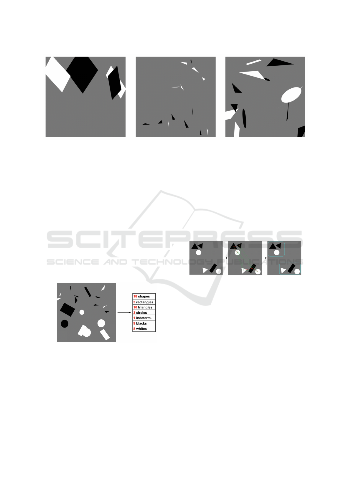
Figure 1: Example compositions from the dataset.

A summary of the designed features that had been

extracted from the compositions is presented below.

3.2.1 Number of Shapes

The feature returns the number of shapes in a compo-

sition.

3.2.2 Number of Speciﬁc Shapes

The feature returns the number of triangles, circles,

rectangles and indeterminable shapes. Indeterminable

shapes may appear on compositions when two or

more shapes overlap.

3.2.3 Number of Speciﬁc Colors

The feature returns the number of black and the num-

ber of white shapes.

Figure 2: Features 1, 2 and 3.

3.2.4 B&W Ratio

The feature returns the ratio between the number of

black and the number of white shapes. The denomi-

nator of the fraction is always the greater number out

of the two. If one of the numbers is zero, the function

returns zero.

3.2.5 Number of Groups

The feature returns the number of groups in a compo-

sition. Groups are subsets of all shapes in which the

shapes are the closest to each other. The function ﬁrst

determines the centers of the shapes, then calculates

the Euclidean distance between every possible pair.

After this step, let’s consider the image as a graph.

Each shape (vertex) is then connected to its closest

neighbor. The number of groups in the composition

is the number of disconnected sub-graphs in the graph

(see Figure 3).

Figure 3: Grouping (Feature 5).

3.2.6 Covered Area

The features returns the ratio between the area cov-

ered by the shapes and the area of the image.

3.2.7 Area Covered by Groups

The feature determines the ratio between the area cov-

ered by each group and the area of the image. Then

the statistical properties of the obtained values are ex-

tracted as mentioned above.

3.2.8 Entropy

The feature returns three numbers that indicate how

much the shapes are spread in a composition; the

more spread they are, the higher its entropy (see Fig-

ure 4). By decreasing the sizes of the squares in

each step, the function ﬁts square grids on the image

multiple times. After every iteration, the number of

Can We Detect Harmony in Artistic Compositions? A Machine Learning Approach

189

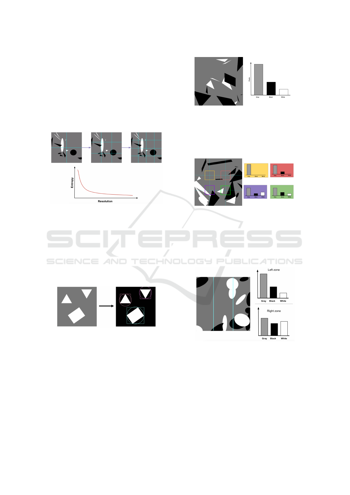
gird cells that contain non-gray pixels are determined.

This number is then divided by number of grid cells in

the current iteration. The result of these divisions are

saved after each step. If we then plot the values, we

get a curve which shows how the entropy decreases

over the iterations. In the last step, a second degree

polynomial is ﬁt to the curve. The function returns

the values of a, b and c determined for the polyno-

mial

+ bx + c (1)

Figure 4: Entropy (Feature 8).

3.2.9 Bounding

The feature ﬁrst ﬁts a bounding circle and a bound-

ing rectangle around every shape in a composition

(see Figure 5. The radiuses of the bounding circles,

and the widths and heights of the bounding rectan-

gles are stored. The function determines the statisti-

cal properties of the list of radiuses, widths, heights,

width/heights and width*heights.

Figure 5: Bounding (Feature 9).

3.2.10 Color Distribution

This feature returns the number of gray, black and

white pixels in an image (see Figure 6).

3.2.11 Two-third Points

This feature divides the image plane into thirds along

both the horizontal and the vertical axes and analyzes

the surrounding of those 4 points where the aforemen-

tioned lines intersect (see Figure 7). The surrounding

is deﬁned as a square whose center is an intersection

Figure 6: Color distribution (Feature 10).

point itself. The function returns the color distribution

of these four areas. The motivation behind the feature

is that the attention of the spectator is mostly drawn

to the surrounding of these points (Amirshahi et al.,

2014).

Figure 7: Two-Third points (Feature 11).

3.2.12 Balance

This feature determines the color distribution in the

left and the right third of the image. This is an indica-

tor about how well the two sides of the composition

are balanced (see Figure 8).

Figure 8: Balance (Feature 12).

3.2.13 Gravity

This feature calculates how much the pairs of shapes

on left and the right side of the composition “pull”

each other, which is another type of indication of bal-

ance in the overall picture. First, the composition is

split into two equal halves, then the center and area

of the each shape are determined. According to New-

ton’s law (Newton, 1987), the occurring gravitational

force between two arbitrary shapes — one belonging

ICAART 2021 - 13th International Conference on Agents and Artiﬁcial Intelligence

190

to the right plane and the other to the left one – is

computed. The gravitational equation is expressed as

F = γ ·

· m

(2)

where F denotes the force between objects m

and

, given their spatial distance r. γ is the gravitational

constant, which in this paper is set to 10

−8

. The mass

of a shape is interpreted as its area (see Figure 9).

Figure 9: Gravity (Feature 13).

3.2.14 Areas

This feature return the statistical properties of the list

of areas of the shapes in a composition.

3.2.15 Shape-center Distance

This feature calculates the distances between the cen-

ter of each shape and the center of the image, then

returns the statistical properties of these values (see

Figure 10).

Figure 10: Shape-Center distance (Feature 15).

3.2.16 SURF Features

In order to obtain a more general representation of a

composition, traditional computer vision techniques

had been applied. After extracting the SURF features

(Bay et al., 2006) from the images, k = 5, 10, 20, 50,

100, 200 and 500 clusters had been created with k-

means. The main idea of SURF is to extract detectors

and descriptors from images which are not susceptible

to rotation, scaling etc. Using the visual bag of words

approach, each row of the extracted SURF matrices

had been assigned to its nearest cluster center. This

way, each composition receives a unique, histogram-

like representation with k bars.

3.2.17 Convolutional Autoencoder

To obtain a more dense representation of the com-

positions, a Convolutional Autoencoder (Masci et al.,

2011) had been trained on 70% of the dataset. If the

reconstructed images look like the original ones, it

means that the encoding layer does carry sufﬁcient

information about the compositions, thus the com-

pressed form of an image can be used as a new fea-

ture. For this purpose, the images had been resized to

100 x 100 pixels. Figure 11 shows some reconstructed

images from the test set. The results indicate that the

encoding layer does carry enough information about

the original images and can be used to generate new

features for the training phase. The encoded images

have the size of 13 x 13 pixels, which gives 169 new

features for a composition.

3.3 Pre-processing

3.3.1 Feature Transformation

In order to improve the performance of the models

to be learnt, the distribution of every feature in the

dataset was checked and subjected to transformations

if needed. Speciﬁcally, in case the distribution of a

feature over the dataset looked like a skewed Gaus-

sian, Box-Cox transform was applied; when a feature

was dominated by a single value, square-rooting was

used, and if the feature followed an exponential dis-

tribution, log transform was applied. In cases where a

feature contained outliers, they were removed. After

transforming the features, the dataset was normalized.

3.3.2 Extending the Dataset

In order to further smooth the dataset some additional

features could be added by performing transforma-

tions on them. Given the polished dataset the fol-

lowing transformations were applied to it: Principal

Component Analysis (PCA) (Jolliffe, 2011) with n =

30 components, and truncated Singular Value Decom-

position (SVD) (Golub and Reinsch, 1971) with n =

9 components. The dataset was then extended by its

own dense representations. Overall, each composi-

tion is represented as a 321 dimensional feature vec-

tor.

Can We Detect Harmony in Artistic Compositions? A Machine Learning Approach

191

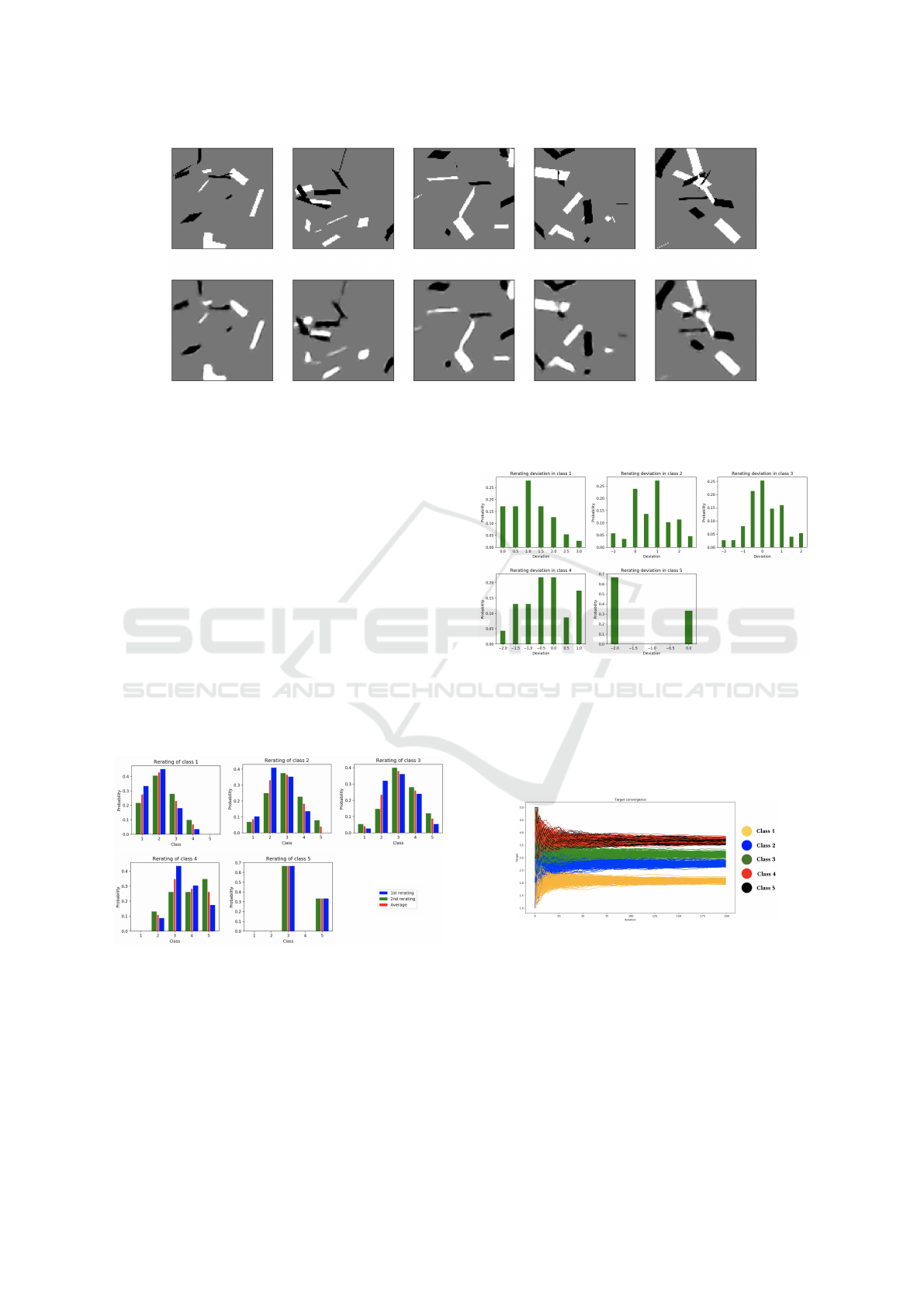
Figure 11: Original (top) and reconstructed (bottom) images.

3.3.3 Fixing the Target Classes

Given the highly subjective nature of the task, we can-

not be certain that participants rate the harmonic na-

ture of the compositions in a consistent way. This

means that we cannot treat the ratings of the compo-

sitions as if they were perfectly expressing their har-

monicity as they experience it. Determining the har-

monicity of a composition may depend on many fac-

tors such the current mood of the participants, which

means they might rate the same images differently in

different situations. In order to smooth out this distor-

tion, participant was asked to re-rate a subset of com-

positions two more times. Provided the re-ratings we

can determine a more robust overall rating for each

composition. Participant was asked to re-rate 300

compositions. Figure 12 shows the deviation from

each class after the re-ratings for the participant.

Figure 12: Re-ratings of participant.

Given the re-ratings, it is possible to determine

how much and how frequently participants deviate

from their initial ratings. Figure 13 shows the dis-

tributions of deviation in each class. For example, in

the second distribution in Figure 13, we can see that

the participant – for the images initially rated as 2’s

– subtracts 1 unit around 5 percent of the time, sub-

tracts 0.5 units around 3 percent of the time, preserves

its rating around 25 percent of the time, adds 0.5 units

around 15 percent of time, and so on.

Figure 13: Distributions of deviation of participant.

By drawing samples from these distributions ac-

cording to the appearing probabilities we can de-

rive what average targets the compositions would get

after several rounds of re-ratings (Bolthausen and

uthrich, 2013). Table 1 shows the resulting values.

Figure 14: Simulated convergence of ratings.

The results of the simulation enable us to assign

new values to the ratings, which express the har-

monicity of compositions more reliably. Table 1 con-

tains the old and the new ratings.

From the converged values we saw that the up-

dated ratings in classes [2, 3] and [4, 5] are fairly

close to each other, so these two class pairs were

merged to describe new categories. Thus, the original

ﬁve classes are merged into three classes, expressing

ICAART 2021 - 13th International Conference on Agents and Artiﬁcial Intelligence

192

the level of harmony in a more compact way: Bad,

Neutral and Good. Table 2 shows the ﬁnal labels used

for training.

Table 1: Converged values.

Old rating New rating

1 2.09

2 2.76

3 3.12

4 3.69

5 3.66

Table 2: Mapping between old and new classes.

Old class New class

1 Bad

2 Neutral

3 Neutral

4 Good

5 Good

3.4 Classiﬁcation Approaches

Given the ﬁnal dataset with all 321 features per com-

position and a clearer notion about what the targets

(classes) represent, we can proceed with applying a

classiﬁcation model on the dataset. We utilized state-

of-the-art machine learning models stemming from

different categories:

• Random Forests (Breiman, 2001) follow the bag-

ging principle and construct multiple (shallow)

decision trees during training time and they pre-

dict the class (in our case the rating) as the mode

of predictions of all trees.

• Gradient Boosting (Friedman, 2001) combines

several weak classiﬁers (in our case decision

trees). The whole idea of boosting is to build

the ﬁnal model step by step: each iteration of the

model is based on a modiﬁed version of the orig-

inal dataset with the goal to reduce the classiﬁca-

tion error of speciﬁc data points. We also employ

XGBoost (Chen and Guestrin, 2016) is a fast and

efﬁcient implementation of gradient boosted deci-

sion trees.

• Logistic Regression (Bishop, 2006) is one of the

most widely used classiﬁcation techniques. We

also employ Ridge classiﬁcation (Hoerl and Ken-

nard, 1970) which can address the multicollinear-

ity issue that large feature spaces suffer from.

• Support Vector Machines (Cortes and Vapnik,

1995) map the input space into separate categories

divided by hyperplanes as wide as possible. Dif-

ferent kernels can be used in order to transform

the non-linear input space into a higher dimen-

sional linear one.

• Multi-layer Perceptrons (Hinton, 1990) are also

used as the simplest feed-forward artiﬁcial neural

network (ANN) for classiﬁcation.

In order to further improve the performance of the

predictions, we combined the above models using

a simple ensemble way (with a naive voting) (Diet-

terich, 2000) and using stacked generalization (which

learns a new model to learn how to best combine the

predictions) (Wolpert, 1992).

In the training phase, all four possible setups were

explored with regards to the targets:

• BN: Bad vs. Neutral,

• BG: Bad vs. Good,

• NG: Neutral vs. Good,

• BNG: using Bad, Neutral and Good classes.

When training the models, each setup was tested with

three different arrangements of the dataset:

• D1: All features are included,

• D2: SURF features are omitted,

• D3: SURF and Convolutional Autoencoder fea-

tures are omitted.

In all setups, 70% of the dataset was used for train-

ing and the remaining 30% for testing. We used 10-

fold cross-validation for all experiments and we fur-

ther used a validation set on the training set to tune

the hyperparameters of all algorithms. Code and data

will be made available upon paper acceptance.

4 EXPERIMENTAL RESULTS

Table 3 summarizes the cross-validated results (accu-

racy and variance) of the best performing (for the sake

of space) models in each setup. The best performance

in each setup is highlighted.

Given the accuracy scores, there are some addi-

tional results which are to be mentioned. Six out of

eight times, the best performing model turned out to

be the SVM, which is in conclusion, the most suited

model for this problem. Along with the SVM, XG-

Boost and Ridge classiﬁers also appear frequently as

best performing models given the different experi-

mental setups. Important to note, that however in the

majority of the cases, stacking yields the best average

accuracy scores, the variance of the accuracies are the

highest. The lowest average variance values belong

to the ensemble setups, indicating that the conﬁdence

Can We Detect Harmony in Artistic Compositions? A Machine Learning Approach

193

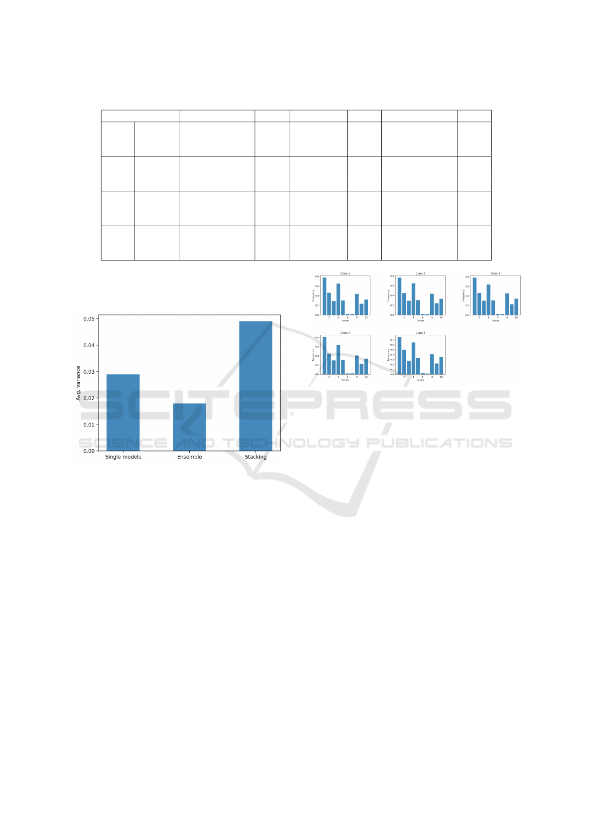
Table 3: Experimental results for all training setups.

Training Setup Single model Var Ensemble Var Stacking Var

D1 0.66 (XGBoost) 0.015 0.65 0.006 0.65 (Ridge) 0.022

BN D2 0.66 (GB) 0.014 0.66 0.007 0.67 (SVM) 0.035

D3 0.66 (XGBoost) 0.008 0.65 0.006 0.64 (XGBoost) 0.017

D1 0.74 (XGBoost) 0.034 0.72 0.017 0.73 (Ridge) 0.06

BG D2 0.73 (XGBoost) 0.029 0.73 0.016 0.80 (SVM) 0.042

D3 0.71 (Ridge) 0.03 0.7 0.02 0.71 (Ridge) 0.058

D1 0.59 (LR) 0.041 0.58 0.03 0.58 (SVM) 0.049

NG D2 0.57 (LR) 0.048 0.56 0.023 0.57 (SVM) 0.063

D3 0.57 (XGBoost) 0.019 0.58 0.022 0.60 (SVM) 0.073

D1 0.48 (XGBoost) 0.023 0.46 0.018 0.47 (Ridge) 0.066

BGN D2 0.47 (GB) 0.029 0.48 0.011 0.50 (SVM) 0.038

D3 0.48 (GB) 0.043 0.47 0.016 0.48 (SVM) 0.041

level rises when combining different models for pre-

dictions. Figure 15 shows the average variances over

different experimental setups.

Figure 15: Average variances over setups.

The least reliable performances were obtained

when using the D1 dataset, which means that the

SURF features do not add to the capturing of the

level of harmony. The fact that the SURF histograms

show signiﬁcant similarities across different classes,

explains why they do not contribute to the predictions.

This outcome is not surprising given the design of

SURF to extract scale- and rotation-invariant interest

point detectors and descriptors which is not desirable

in this type of research. Figure 16 shows averaged

SURF histograms for the original 5 classes with k =

10 cluster centers.

The best mean accuracy (0.80) was obtained using

the BG setup with stacked generalization on the D2

dataset. We can see that the ensemble models made

the predictions more conﬁdent and the stacking man-

aged to further increase mean accuracy.

Figure 16: Average frequencies of SURF features for k =

10 cluster centers across 5 classes.

5 CONCLUSION

The goal of this paper is to explore whether the

subjective perception of harmony can be expressed

numerically. The results show that given a sufﬁ-

ciently large collection of randomly generated black

and white images and the above described features,

there exists an experimental setup by which it is pos-

sible for a machine learning model to distinguish be-

tween Good and Bad compositions with 80% accu-

racy. However, the performance of the models de-

creased when all three classes were involved. That

shows that when separating between classes being

most distant in their level of harmony, it is possible to

assign numerical values to subjectively judged com-

positions in order for an algorithm to conﬁdently clas-

sify them. Given the experimental results, we con-

clude that the SVM and XGBoost classiﬁers are the

most suited for this problem.

The research described here opens several inter-

esting future directions. Among them are, in partic-

ular, the design of more sophisticated and more ex-

pressive features, the collection and pre-processing of

more data from more participants, the extension of the

type and style of artistic compositions, and the explo-

ICAART 2021 - 13th International Conference on Agents and Artiﬁcial Intelligence

194

ration of different scales for rating. Furthermore, the

research introduces the need for interdisciplinary col-

laboration (e.g. by actively involving artists), serving

as a bridge between feature design and art.

REFERENCES

Amirshahi, S. A., Hayn-Leichsenring, G. U., Denzler, J.,

and Redies, C. (2014). Evaluating the rule of thirds

in photographs and paintings. Art & Perception, 2(1-

2):163–182.

Bay, H., Tuytelaars, T., and Van Gool, L. (2006). SURF:

Speeded up robust features. In European conference

on computer vision, pages 404–417. Springer.

Bharati, M. H., Liu, J. J., and MacGregor, J. F. (2004).

Image texture analysis: methods and comparisons.

Chemometrics and intelligent laboratory systems,

72(1):57–71.

Bishop, C. M. (2006). Pattern recognition and machine

learning. springer.

Bolthausen, E. and W

uthrich, M. V. (2013). Bernoulli’s law

of large numbers. ASTIN Bulletin, 43(2):73–79.

Breiman, L. (2001). Random forests. Machine learning,

45(1):5–32.

Chen, T. and Guestrin, C. (2016). Xgboost: A scalable

tree boosting system. In Proceedings of the 22nd acm

sigkdd international conference on knowledge discov-

ery and data mining, pages 785–794. ACM.

Cortes, C. and Vapnik, V. (1995). Support-vector networks.

Machine learning, 20(3):273–297.

Davis, R. C. (1936). An evaluation and test of birkhoff’s

aesthetic measure formula. The Journal of General

Psychology, 15(2):231–240.

Deepa, S. and Devi, B. A. (2011). A survey on artiﬁ-

cial intelligence approaches for medical image clas-

siﬁcation. Indian Journal of Science and Technology,

4(11):1583–1595.

Di Dio, C., Macaluso, E., and Rizzolatti, G. (2007). The

golden beauty: brain response to classical and renais-

sance sculptures. PloS one, 2(11):e1201.

Dietterich, T. G. (2000). Ensemble methods in machine

learning. In International workshop on multiple clas-

siﬁer systems, pages 1–15. Springer.

Friedman, J. H. (2001). Greedy function approximation: a

gradient boosting machine. Annals of statistics, pages

1189–1232.

Golub, G. H. and Reinsch, C. (1971). Singular value de-

composition and least squares solutions. In Linear Al-

gebra, pages 134–151. Springer.

Hinton, G. E. (1990). Connectionist learning procedures. In

Machine learning, pages 555–610. Elsevier.

Hoerl, A. E. and Kennard, R. W. (1970). Ridge regression:

Biased estimation for nonorthogonal problems. Tech-

nometrics, 12(1):55–67.

Jolliffe, I. (2011). Principal component analysis. Springer.

Jordanous, A. (2012). A standardised procedure for evalu-

ating creative systems: Computational creativity eval-

uation based on what it is to be creative. Cognitive

Computation, 4(3):246–279.

LeCun, Y., Boser, B. E., Denker, J. S., Henderson, D.,

Howard, R. E., Hubbard, W. E., and Jackel, L. D.

(1990). Handwritten digit recognition with a back-

propagation network. In Advances in neural informa-

tion processing systems, pages 396–404.

Leder, H., Belke, B., Oeberst, A., and Augustin, D. (2004).

A model of aesthetic appreciation and aesthetic judg-

ments. British journal of psychology, 95(4):489–508.

Lowe, D. G. (1999). Object recognition from local scale-

invariant features. In Computer vision, 1999. The pro-

ceedings of the seventh IEEE international conference

on, volume 2, pages 1150–1157. Ieee.

Masci, J., Meier, U., Cires¸an, D., and Schmidhuber, J.

(2011). Stacked convolutional auto-encoders for hi-

erarchical feature extraction. In International Con-

ference on Artiﬁcial Neural Networks, pages 52–59.

Springer.

Newton, I. (1987). Philosophiæ naturalis principia math-

ematica (mathematical principles of natural philoso-

phy). London (1687), 1687.

Nixon, M. and Aguado, A. S. (2012). Feature extraction

and image processing for computer vision. Academic

Press.

Pappas, N. (2008). Plato’s aesthetics.

ping Tian, D. et al. (2013). A review on image feature ex-

traction and representation techniques. International

Journal of Multimedia and Ubiquitous Engineering,

8(4):385–396.

Salleh, N. D. H. M. and Phon-Amnuaisuk, S. (2015). Quan-

tifying aesthetic beauty through its dimensions: a case

study on trochoids. International Journal of Knowl-

edge Engineering and Soft Data Paradigms, 5(1):51–

64.

Wolpert, D. H. (1992). Stacked generalization. Neural net-

works, 5(2):241–259.

Wu, S. G., Bao, F. S., Xu, E. Y., Wang, Y.-X., Chang, Y.-F.,

and Xiang, Q.-L. (2007). A leaf recognition algorithm

for plant classiﬁcation using probabilistic neural net-

work. In Signal Processing and Information Technol-

ogy, 2007 IEEE International Symposium on, pages

11–16. IEEE.

Zhao, W., Krishnaswamy, A., Chellappa, R., Swets, D. L.,

and Weng, J. (1998). Discriminant analysis of princi-

pal components for face recognition. In Face Recog-

nition, pages 73–85. Springer.

Can We Detect Harmony in Artistic Compositions? A Machine Learning Approach

195