Efﬁcient Image Registration with Subpixel Accuracy using a Hybrid

Fourier-based Approach

Jelina Unger and Klaus Brinker

Hamm-Lippstadt University of Applied Sciences, Marker Allee 76-78, 59063 Hamm, Germany

Keywords:

Image Registration, Fourier-based Cross Correlation, Image Projections, Subpixel Accuracy.

Abstract:

In many ﬁelds like medical imaging and remote sensing, it is necessary to register images with subpixel accu-

racy. A general problem is the tradeoff between accuracy and efﬁciency. This paper presents a highly accurate

and efﬁcient algorithm for subpixel image registration using Fourier-based cross correlation to determine the

translation between two images. Therefore a coarse to ﬁne strategy is used. It combines a fast method using

image projections with an accurate approach using matrix multiplication for reﬁned computation. The results

show that the new approach has almost the same level of accuracy as the accurate method, but with reduced

computational complexity. Compared to the fast method, the computational complexity of the new approach

is slightly higher, but achievs a higher level of accuracy. Overall the hybrid approach achieves an efﬁcient

registration with a relatively short runtime.

1 INTRODUCTION

Image registration is the process of aligning two or

more images of the same object on top of each other.

For this purpose the transformation between those im-

ages is determined. Typical transformation types are

rotation, scaling, and translation. In this paper we

focus on translations which is suitable, e.g. for mi-

croscopic applications among others. Many applica-

tions require calculation of the transformation down

to a fraction of a pixel, i.e. with subpixel accuracy.

In medical imaging, this allows monitoring changes

in the human body of one patient but also facilitates

comparing different patients. For this purpose images

of different times or modalities are registered (Farn-

combe and Iniewski, 2014).

Fourier-based methods have gained increasing at-

tention in recent years. The basic method is to com-

pute an upsampled version of the cross correlation be-

tween two images using the discrete Fourier Trans-

form (DFT) and locate its peak. In general, the main

problem is to exhibit high accuracy and low com-

putational time simultaneously (Tong et al., 2019).

Guizar-Sicairos et al. (2008) present a highly accu-

rate approach. A coarse to ﬁne strategy is imple-

mented using matrix multiplication to be more efﬁ-

cient. Still, this approach yields a high computational

complexity. A fast approach is presented by Yang et

al. (2012). They only use image projections which

reduces the runtime but also decreases the level of ac-

curacy. The aim of the present work is to combine

both approaches to one highly efﬁcient and accurate

hybrid algorithm.

Section 2 presents the basic methods of Fourier-

based image registration and outlines the three al-

gorithms. In Section 3, an evaluation of the algo-

rithms and different relevant inﬂuencing factors are

presented. The results are discussed in Section 4. Fi-

nally a conclusion is given in Section 5.

2 REGISTRATION METHODS

In the following, we ﬁrst introduce the deﬁnitions of

the DFT, explain the basic method for subpixel image

registration, and lastly present the three algorithms.

The DFT and its inverse can be calculated by dif-

ferent methods. In this paper the transformation for-

mula and matrix multiplication are used. The trans-

formation formula for 1D-DFT of a signal f(x) with

length N is shown in Equation 1 (McAndrew, 2016).

F(u) =

N−1

∑

x=0

f (x)exp

−2πi

(1)

The inverse 1D-DFT of the Fourier-Spectral F(u) can

be calculated using Equation 2.

f (x) =

N−1

∑

u=0

F(u)exp

2πi

(2)

Images can be described as a two-dimensional func-

tion F(x,y) with dimensions N × M. Therefore, the

136

Unger, J. and Brinker, K.

Efﬁcient Image Registration with Subpixel Accuracy using a Hybrid Fourier-based Approach.

DOI: 10.5220/0010242901360143

In Proceedings of the 14th International Joint Conference on Biomedical Engineering Systems and Technologies (BIOSTEC 2021) - Volume 2: BIOIMAGING, pages 136-143

ISBN: 978-989-758-490-9

generalized 2D-DFT formula is necessary, which is

shown in Equation 3.

F(u, v) =

N−1

∑

x=0

M−1

∑

y=0

f (x, y)exp

−2πi



o

(3)

The inverse 2D-DFT is calculated by Equation 4.

f (x, y) =

N−1

∑

u=0

M−1

∑

v=0

F(u, v)exp

2πi



o

(4)

Matrix multiplication is another method to calcu-

late the (inverse) 2D-DFT of images (Soummer et al.,

2007). It can be expressed as

F(u, v) = w

· f (x, y) · w

(5)

and

f (x, y) =

∗

· F(u, v) ·

∗

(6)

where w

and w

are the transformation matrices

and * indicates the complex conjugation. They are

deﬁned by Equation 7 and 8.

= exp

{

−2πiXU

}

(7)

= exp

{

−2πiYV

}

(8)

The vectors X and U are deﬁned as

X =

(

[0, 1, ..., N − 1] −

for even N

[0, 1, ..., N − 1] −

N−1

for odd N

(9)

and

U =

(

· [0, 1, ...,

− 1, −

, ..., −1] for even N

· [0, 1, ...,

N−1

, −

N−1

, ..., −1] for odd N

(10)

where N describes the height of the image. Y and V

are computed analogously but with the exception that

image width M replaces height N.

2.1 Subpixel Image Registration

In general, the translation between two images f(x,y)

and g(x,y) can be described as

f (x, y) = g(x − ∆x, y − ∆y) (11)

where ∆x and ∆y are the vertical and the horizontal

shifts (Tong et al., 2019). We deﬁne f as the refer-

ence image and g as the image to be registered. To

compute these translations, Fourier-based cross cor-

relation is computed by Equation 12 and its peak has

to be located (Anuta, 1970).

CC(x, y) = F

−1

(F(u, v)G

∗

(u, v)) (12)

G and F denote the Fourier-Transform of images g

and f, * indicates the complex conjugation and F

−1

the inverse DFT. For achieving subpixel accuracy, an

upsampled version of the cross correlation is required.

Therefore, the number of data points is increased by

a factor of κ, allowing a theoredical accuracy of

a pixel. A common method to achieve upsampling is

zero-padding (Shin et al., 2017). For this, the prod-

uct F(u, v)G

∗

(u, v) with size N × M is embedded in

a larger array of zeros with size κN × κ M. Calculat-

ing the inverse DFT of this array results in an upsam-

pled version of the cross correlation. Finally the peaks

are located and the shifts are converted to the original

pixel units (Yang et al., 2012).

Another method to perform upsampling is to cal-

culate the inverse DFT by using matrix multiplication.

For this, the transformation matrices must be adjusted

by increasing the value range of the vectors X, Y, U

and V by the upsampling factor κ. Furthermore, the

upsampling can be limited to a speciﬁc image region.

The vector X is computed by

X =

(

[0, 1, ..., Dκ − 1] −

Dκ

+ sκ for even Dκ

[0, 1, ..., Dκ − 1] −

Dκ−1

+ sκ for odd Dκ

(13)

where D denotes the image region height and s the

vertical center. Y is computed analogously with the

exception that the width replaces the height and the

horizontal replaces the vertical center. To calculate

the vector U Equation 14 is used.

U =

(

κN

· [0, 1, ...,

− 1, −

, ..., −1] for even N

κN

· [0, 1, ...,

N−1

, −

N−1

, ..., −1] for odd N

(14)

To compute V, the same approach can be used by

replacing the height N with the width M (Soummer

et al., 2007).

Due to the increase of data points, the upsampling

is always related to a higher computational complex-

ity. The advantage of the matrix multiplication is that

the upsampling can be localized to a speciﬁc image

region (Tong et al., 2019).

2.2 Matrix Multiplication DFT

Approach

A highly accurate algorithm to register images by us-

ing Fourier-based cross correlation is presented by

Guizar-Sicairos et al. (2008). A coarse to ﬁne strat-

egy is used. The ﬁrst step is to compute the Fourier-

based cross correlation over the entire image using

zero-padding with an upsampling factor of κ

= 2 and

to locate its peak. In the second step, an upsampled

version of the 1.5 × 1.5 pixel neighborhood around

the rough estimation is computed by matrix multi-

plication. At this point the upsampling factor is ad-

justable. The peak is located in the output array and

Efﬁcient Image Registration with Subpixel Accuracy using a Hybrid Fourier-based Approach

137

converted into units of original pixels. The last step

is to combine the rough and reﬁned estimation to the

ﬁnal translation vector. We refer to this algorithm as

MM.

2.3 Image Projections DFT Approach

A high-speed algorithm for subpixel image registra-

tion is presented by Yang et al. (2012). To reduce

computational time, one-dimensional image projec-

tions are used to compute the upsampled Fourier-

based cross correlations.

First, vertical and horizontal image projections are

calculated by taking the sum of each row respectively

column, using Equation 15 and 16 for an image f(x,y)

with height N and width M.

row

(x) =

M−1

∑

y=0

f (x, y) (15)

col

(y) =

N−1

∑

x=0

f (x, y) (16)

The information of edges can inﬂuence the cross cor-

relation. To reduce this effect a ﬁlter is applied, which

is shown in Equation 17 and 18.

row, f ilt

(x) = f

row

(x) −

N−1

∑

i=0

row

(i)

(17)

col, f ilt

(y) = f

col

(y) −

M−1

∑

j=0

col

( j)

(18)

This preprocessing step is performed for both

images f(x,y) and g(x,y). All ﬁltered projections

are transformed in the frequency domain by using

the transformation formula. Hence, two products

row

(u)G

∗

row

(u) and F

col

(v)G

∗

col

(v) are computed. In

order to achieve subpixel accuracy, zero-padding is

used. For this purpose both products are embedded in

larger arrays of zeros with size κN respectively κM.

Computing the inverse 1D-DFT with the transforma-

tion formula of these arrays results in upsampled ver-

sions of cross correlations. Finally peaks are located

and converted into units of original pixels to receive

vertical and horizontal translations. We refer to this

algorithm as IP.

2.4 Combination of Image Projections

and Matrix Multiplication DFT

In this paper we present a novel efﬁcient algorithm

which combines the MM algorithm from (Guizar-

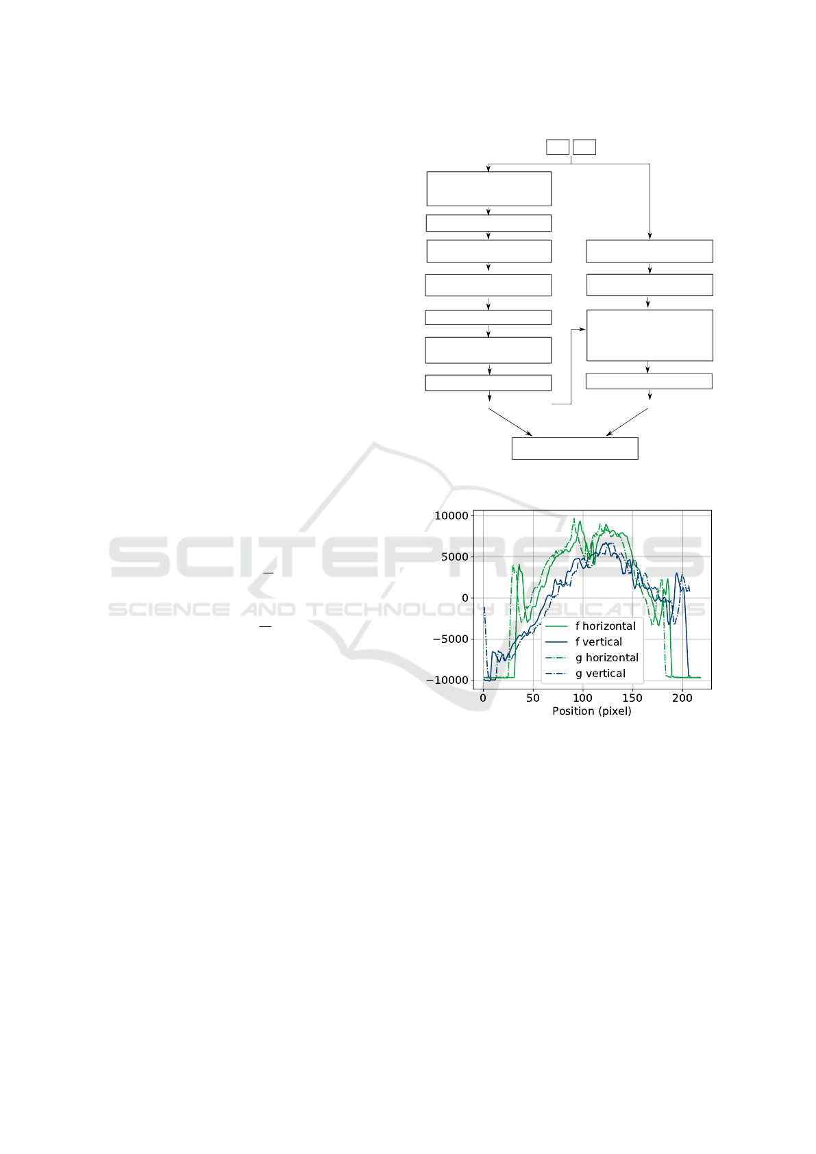
Sicairos et al., 2008) and the IP algorithm from (Yang

Horizontal & vertical

image projections

row

, f

col

, g

row

, g

col

Filter projections

1D DFT of projections

row

, F

col

, G

row

, G

col

Projections product

row

* and F

col

Zero padding with �

= 2

1D cross correlations

by computing inverse DFT

Locate peaks

Rough estimation of translation

2D DFT of images

F and G

Image product

FG*

Upsampled 2D cross correlation

over rough translation estimation

by computing inverse DFT

using matrix multiplication

Locate peak

Refined translation

Combine rough and refined

translation values

Images

Figure 1: Computational process of the proposed combina-

tion approach.

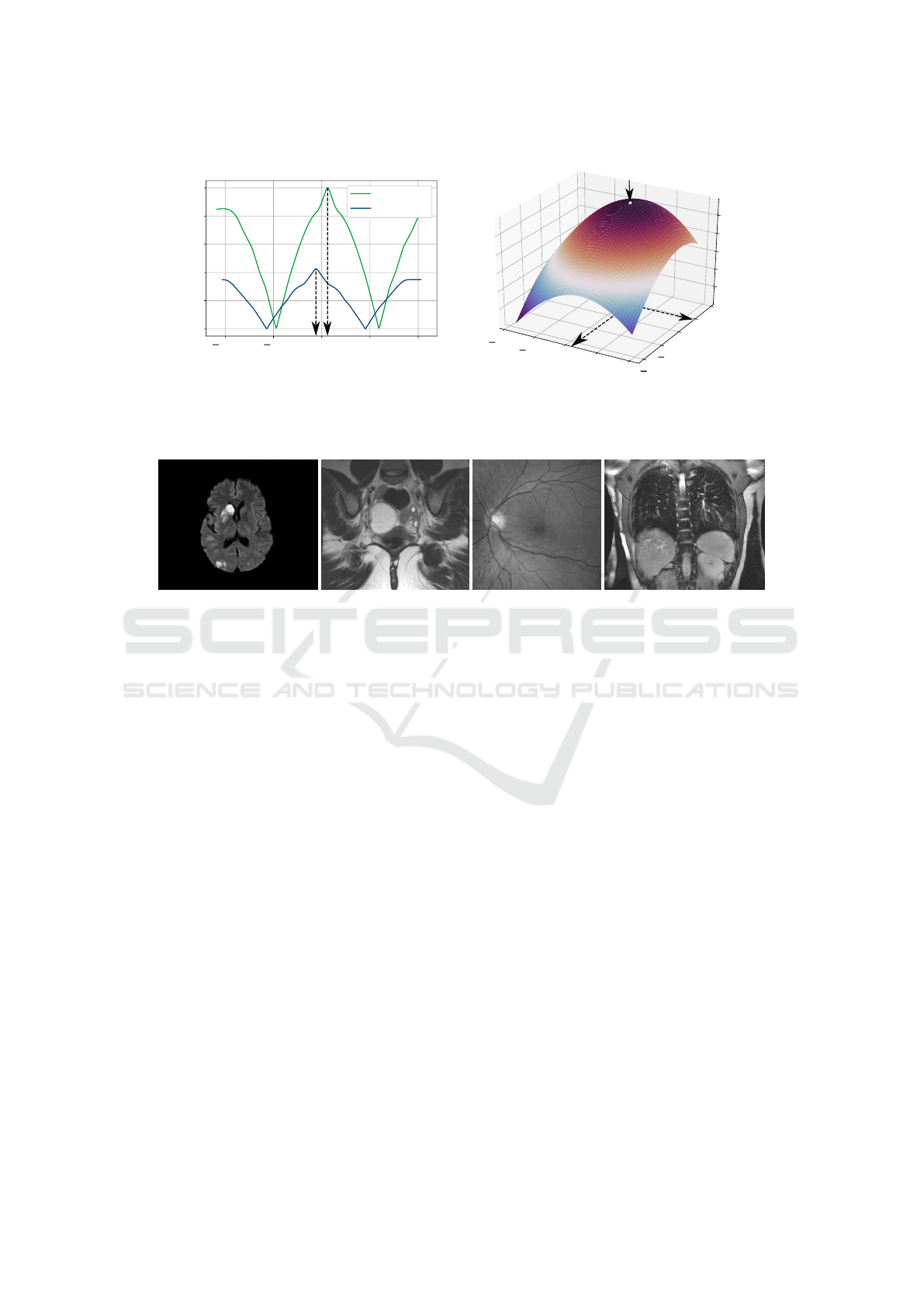
Figure 2: Filtered image projections for the reference image

f and the image to be registered g.

et al., 2012). The main idea is to keep the high ac-

curacy of MM, but with low computational time like

IP. Therefore, we consider a coarse to ﬁne strategy.

For the ﬁrst rough estimation, the IP approach is used

with an upsampling factor of κ

= 2. MM is used for

the reﬁned estimation of translation. A more detailed

computational process visualization is given in Fig-

ure 1 and explained in the following. This steps are

performed for two images f(x,y) and g(x,y):

1. Rough shift estimation

(a) compute and ﬁlter vertical and horizontal pro-

jections of both images

(b) compute upsampled Fourier-based cross cor-

relations of vertical and horizontal projections

BIOIMAGING 2021 - 8th International Conference on Bioimaging

138

100 50 0 50 100

Translation (pixel)

0.0

0.2

0.4

0.6

0.8

1.0

Cross correlation

1e10

horizontal

vertical

(a)

Vertical translation

(pixel)

0.8

0.4

0.0

0.4

0.8

Horizontal translation

(pixel)

0.8

0.4

0.0

0.4

0.8

Cross correlation

(b)

Figure 3: Visualization for the main steps of combination algorithm: (a) 1D rough cross correlations and (b) 2D reﬁned cross

correlation around the rough estimation, where the locations of peaks are marked by arrows.

Figure 4: Four examples of test images from (He et al., 2020), (Budai et al., 2013) and (Cohen, 2020).

with an upsampling factor of κ

= 2 by using

zero-padding and transformation formula

units

2. Reﬁned shift estimation

(a) compute the product F(u, v)G

∗

(u, v) and deﬁne

transformation matrices w

and w

for im-

age region centered over the rough estimated

peak with a region size of 1.5κ × 1.5κ pixel in

upsampled pixel units

(b) compute the upsampled cross correlation by

multiplying these three matrices

units

3. Add rough and reﬁned estimation for receiving

the total translation vector

The ﬁltered image projections are visualized in

Figure 2. It can be seen that projections of the image g

have the same shape as the reference image f, but are

shifted slightly. Figure 3 shows the cross correlations

for the ﬁrst rough and the reﬁned estimation. The

rough estimation consists of two one-dimensional

cross correlations for the vertical and horizontal di-

rection. Their peaks can clearly be determined for -6

and 6 pixels. The reﬁned cross correlation over the

rough estimation has a peak at (0.32, 0.10). For both

cross correlation plots, peaks and their corresponding

position are marked by arrows. In total a translation

of (−5.68, 6.10) is determined for this sample image

pair by adding rough and reﬁned estimation.

2.5 Implementation

All three algorithms were implemented in Python

(version 3.7.1). Standard libraries especially NumPy

(version 1.18.1) and its modul numpy.fft for discrete

Fourier Transform were used. The library Scikit-

image (version 0.16.2) was only used for loading im-

ages. For the MM approach the implementations from

(Guizar, 2016) and (Fezzani et al., 2020) were used.

Evaluation is performed on a HP 250 G5 Notebook

with Intel(R) Core Processor 2.40 GHz, 8 GB RAM

and 64-bit-operating-system.

3 EVALUATION

In this section, we evaluate all three algorithms with

respect to accuracy and runtime. First, the methods

for conducting the evaluation are described. Further

on, the general performance for accuracy and runtime

is evaluated. Additionally, we analyze performance

for different image sizes and under the presence of

Efﬁcient Image Registration with Subpixel Accuracy using a Hybrid Fourier-based Approach

139

(a) (b) (c) (d)

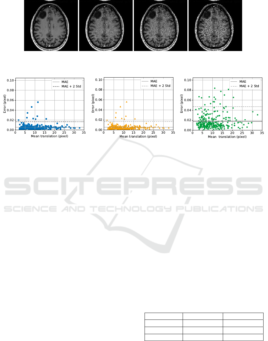
Figure 5: Visualization of different noise variances for a test image (He et al., 2020): (a) 0, (b) 0.05 (c) 0.1 and (d) 0.3.

(a)

(b)

(c)

Figure 6: Visualization of the pixel error versus mean translation for (a) MM, (b) combination algorithm and (c) IP.

noise. The ﬁnal part of the evaluation includes an

analysis of the inﬂuence of different upsampling fac-

tors.

3.1 Methods

For the evaluation, a dataset of 300 medical images

from (He et al., 2020), (Budai et al., 2013) and (Co-

hen, 2020) is used for the reference images. Four

sample images are shown in Figure 4. In order to

obtain an image to be registered for each reference

image, a random translation is performed which is be-

tween 0.5 % and 3 % of the corresponding image side.

Additionally, noise is added to slightly change the im-

age information in contrast to the reference image.

To evaluate the accuracy, the mean value is calcu-

lated from the absolute vertical and horizontal error

for each image pair. Additionally, the mean absolute

error (MAE) is calculated over the entire dataset in or-

der to assess general performance. Furthermore, the

runtime is measured and the mean value is calculated

over the dataset to evaluate the efﬁciency. The tol-

erances are given by the doubled standard deviation

(Std).

For the ﬁrst three parts of evaluation, an upsam-

pling factor of κ = 100 is used. In order to ana-

lyze the performance with noisy images, the dataset

is extended. The same translations as for the ﬁrst

three parts are used, but six images to be registered

with different noise levels for every reference im-

age are created. A multiplicative Gaussian noise is

used. The noisy image is deﬁned as image

noise

image + n ∗ image, where n is Gaussian noise with

zero mean and different variances in the range of 0

to 0.3. In Figure 5, four noise levels are shown by a

sample test image.

3.2 General Performance

The results for the general performance of all algo-

rithms are shown in Table 1. The MM and combina-

tion algorithm have the same high level of accuracy of

0.005 ± 0.011 pixel for the MAE. The MAE of the IP

approach is more than three times as large. But the IP

method has the shortest runtime with 0.019 ± 0.029 s.

The combination algorithm is just slightly slower, but

MM requires signiﬁcantly more time. Accordingly,

the combination algorithm reduces the MAE in con-

trast to the IP approach by over 70 % and runtime in

contrast to the MM approach by over 75 %.

Table 1: General performance for all algorithms.

Algorithm MAE (pixel) Runtime (s)

MM 0.005 ± 0.011 0.324 ± 0.562

Combination 0.005 ± 0.011 0.079 ± 0.125

IP 0.017 ± 0.029 0.019 ± 0.029

The results for the error in dependence on trans-

lation are visualized in Figure 6. Besides, the MAE

the limit of tolerance for the dataset is given. It is

shown that most error samples for MM and combina-

BIOIMAGING 2021 - 8th International Conference on Bioimaging

140

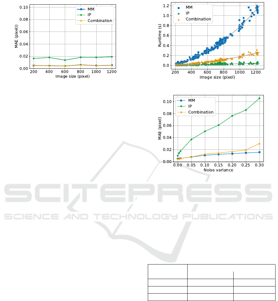
Figure 7: MAE depending on image size.

tion are within this limit. For the IP, the tolerance limit

is larger and error samples spread more. Furthermore,

the error is equally distributed over the translation size

for all algorithms, therefore, no dependence between

error and size of translation is visible here.

3.3 Dependency on Image Size

In the following, we analyze whether image size in-

ﬂuences accuracy and runtime. To visualize accu-

racy, the images were grouped by size and the MAE

were calculated for each group (Figure 7). As already

shown in Section 3.2, the MAE for the IP approach is

clearly higher than for the other two algorithms. The

MAE for the MM and combination approach is ex-

actly the same. However, for all algorithms the MAE

is about the same for all sizes. There are only minor

ﬂuctuations that don’t indicate a clear trend. Hence,

no dependency can be determined.

Though, a clear dependency on the image size

for the runtime can be determined, which is shown

in Figure 8. The runtime increases with larger im-

age size. For small images around 200 pixel im-

age dimension, all algorithms have a low runtime

under 0.04 s. But the runtime of the MM approach

is already slightly higher. Additionally it shows the

sharpest increase with a quadratic trend up to 1.2 s.

The runtime of the combination approach also shows

a quadratic trend, but the curve progression is much

ﬂatter though, reaching a maximum of only 0.26 s

which is almost 80 % less than the MM. The IP ap-

proach shows only a slight linear increase in time up

to 0.045 s.

3.4 Dependency on Noise

In the following we analyze the performance for im-

ages with different noise levels. Figure 9 shows the

MAE at different noise levels. The MM and combina-

tion approach achieve low MAE. The MM approach

has a slight linear increase of the MAE from 0.005

Figure 8: Runtime depending on image size.

Figure 9: MAE depending on noise variance.

up to 0.015 pixel. For low noise levels the combina-

tion algorithm has the same accuracy as MM. Though

starting from the noise variance of 0.1, the MAE in-

creases slightly more up to 0.03 pixel. In contrast,

the MAE of IP already rises steeply for low noise lev-

els from 0.009 to 0.106 pixel. For the highest noise

level, the MAE of the combination algorithm is twice

as large as of the MM, but still 70 % less than of the

IP approach.

Table 2: MAE for general performance and noisy images.

Algorithm MAE (pixel)

normal images noisy images

MM 0.005 ± 0.011 0.010 ± 0.018

Combination 0.005 ± 0.011 0.013 ± 0.052

IP 0.017 ± 0.029 0.051 ± 0.172

In comparison to the general performance, which

is presented in Section 3.2, the MAE of subpixel ac-

curacy increases for all algorithms (Table 2). For MM

and combination the MAE doubles, but for the com-

bination the increase is slightly more. For the IP a

steep increase can be observed. Moreover, the MAE

is tripled. For normal images the error of the combi-

nation algorithm is 70 % less compared to IP and even

75 % for noisy images.

Efﬁcient Image Registration with Subpixel Accuracy using a Hybrid Fourier-based Approach

141

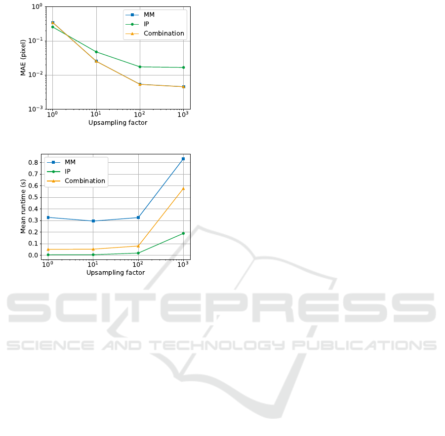
Figure 10: MAE depending on upsampling factor.

Figure 11: Runtime depending on upsampling factor.

3.5 Dependency on the Upsampling

Factor

In the following, the inﬂuence of different upsampling

factors to subpixel accuracy and runtime is evaluated.

If the upsampling factor is increased by a factor of

10, the registration is theoretically more accurate by

a factor of 10. However, Figure 10 shows that this is

not always the case. For the IP, the decrease of MAE

becomes less and from upsampling factor 100 to 1000

it totally stagnates. The MAE for MM and combina-

tion is exactly the same. In the beginning it decreases

almost by a factor of 10. But for κ = 1000 it also stag-

nates.

At values of κ = 1, which means there is no up-

sampling, IP is slightly more accurate. But for higher

values, the MAE of MM and the combination ap-

proach is signiﬁcantly less. For the κ = 10, it is al-

ready 20 % and for κ = 100 and κ = 1000 it is more

than 70 %.

Taking runtime into account, it can be observed

that there are only slight changes for the ﬁrst three

upsampling factors 1 to 100, but for the highest fac-

tor runtime increases rapidly (Figure 11). Gener-

ally, the IP approach has the shortest runtime with

0.008 ± 0.03 s for an upsampling with the factor 1 to

100 and increases by 0.18 s for the highest factor. The

MM approach has a considerably longer runtime with

0.315 ± 0.648 s for lower upsampling factors and in-

creases more rapidly for the highest upsampling by

0.517 s. The runtime for the combination algorithm is

slightly higher than for the IP, but signiﬁcantly lower

than for the MM with 0.060 ± 0.126 s for the lower

upsampling factors. Though it increases by 0.516 s

for the highest upsampling as the MM approach.

4 DISCUSSION

The purpose of this paper was to combine two image

registration algorithms so that the translation between

images can be determined with high accuracy and low

computational requirements. The results have shown

that our combination algorithm fulﬁlls these two cri-

teria. The MM approach is always the most accurate

one, but the combination algorithm achieves almost

the same level of accuracy. In contrast, the IP has al-

ways a signiﬁcantly higher error. However, regarding

runtime it is the most efﬁcient. The combination al-

gorithm can’t achieve the same low runtime, but it is

still in a very low range of a few milliseconds. Espe-

cially compared to the MM approach, runtime can be

reduced signiﬁcantly. Additionally, the combination

algorithm isn’t as sensitive to large image sizes. As

seen in Figure 8, the runtime of the combination in-

creases signiﬁcantly less than for the MM approach.

Hence, the dependency on the image size is low and

therefore it is applicable to scenarios with large image

dimensions.

We conclude that accuracy of all algorithms

doesn’t depend on translation and image size. As we

only conducted limited experiments regarding the im-

age and translation size, it can not be ruled out that the

accuracy is dependent on translations, especially large

ones. Because the larger the translation, the smaller

the matching image regions. Thus, the similarity be-

tween both images is reduced, which could compli-

cate the registration process. However as such large

translation are rare in medicine, we choose this set-

ting.

Guizar-Sicairos et al. (2008) states that the MM

approach is robust to noise, because the whole image

information is used for the rough estimation and all

data points from the upsampled cross correlation as

well. Our results conﬁrm these ﬁndings as seen in

Figure 9. The IP doesn’t use the whole image infor-

mation, because due to image projections the data is

reduced. Hence, it is highly sensitive to noise. The

combination algorithm is to a similar degree as MM

robust to noise. Just for high noise levels it is slightly

more sensitive. Conducting the ﬁrst rough estimation

by the projection method is mostly accurate enough.

BIOIMAGING 2021 - 8th International Conference on Bioimaging

142

If the real peak is still within proximity to the ﬁrst es-

timation, the reﬁned estimation can still recover it. If

the rough estimation is very imprecise, an unavoid-

able error will occur in the reﬁned determination. To

improve the algorithm in this respect, the rough esti-

mation can be reﬁned by using a higher upsampling

factor or to enlarge image region for the reﬁned esti-

mation. For this reason, it must be clariﬁed whether

the gain in accuracy is worth the increase in runtime.

The upsampling factor is a tool to achieve higher

accuracy. For a factor κ translation can be determined

of a pixel. Results have shown that this factor

is limited to 100. Higher factors don’t achieve higher

accuracy. Additionally, a higher upsampling results in

a longer runtime, because there are more data points

to be processed. For low factors the increase in run-

time isn’t signiﬁcant, because it’s just a slight increase

of data. However, for large factors like 1000 run-

time increases rapidly. This property was observed

for all algorithms. Finally an upsampling factor of

κ = 100 is a suitable choice, because best accuracy

can be achieved without rapid increase of runtime.

The combination algorithm is limited to determine

translation between images. Therefore, our evalua-

tion only focuses on paraxial translation between im-

ages. For most image registration problems, rotation

and scaling has to be considered as additional trans-

formations between images. In order to generalize our

algorithm it can be extended to determine also other

transformations: The Fourier-Mellin-Transformation

can be used for computing rotation and scaling, and

afterwards determining the translation (Tong et al.,

2019).

5 CONCLUSIONS

This paper presents an efﬁcient algorithm for image

registration with subpixel accuracy. More precisely,

we propose a hybrid approach consisting of a coarse

to ﬁne strategy. For the ﬁrst rough estimation image

projections are used, while for the reﬁned estimation

the method of matrix multiplication is performed only

on a small region around the ﬁrst estimation center.

Experimental results have shown that the algorithm

is very accurate and computationally highly efﬁcient.

The MAE can be reduced by over 70 % compared to

the IP approach and runtime by over 75 % compared

to the MM approach. It is robust with respect to noise

and can handle large images. To improve the algo-

rithm in further work, it can be extended to consider

generalized transformation models, such as including

rotation and scaling.

REFERENCES

Anuta, P. (1970). Spatial registration of multispectral and

multitemporal digital imagery using fast fourier trans-

form techniques. IEEE Transactions on Geoscience

Electronics, 8(4):353–368.

Budai, A., Bock, R., Maier, A., Hornegger, J., and Michel-

son, G. (2013). Robust vessel segmentation in fundus

images: High-resolution fundus image dataset. Inter-

national Journal of Biomedical Imaging.

Cohen, J. (2020). Covid chest x-ray dataset. Avail-

able: https://github.com/ieee8023/covid-chestxray-

dataset. (visited on July 22, 2020).

Farncombe, T. and Iniewski, K. (2014). Medical imaging:

Technology and applications. Devices, circuits, and

systems. CRC Press, Boca Raton, Fla.

Fezzani, R., Nunez-Iglesias, J., Lee, G. R., and Boulogne,

F. (2020). scikit-image phase cross correlation.

Available: https://github.com/scikit-image/scikit-

image/blob/v0.17.2/skimage/registration/ phase

cross correlation.py. (visited on August 08, 2020).

Guizar, M. (2016). Efﬁzient subpixel image registration by

cross-correlation. Available: https://www.mathworks.

com/matlabcentral/ﬁleexchange/18401-efﬁcient-

subpixel-image-registration-by-cross-correlation.

(visited on August 08, 2020).

Guizar-Sicairos, M., Thurman, S. T., and Fienup, J. R.

(2008). Efﬁcient subpixel image registration algo-

rithms. Optics letters, 33(2):156–158.

He, X., Zhang, Y., Mou, L., Xing, E., and Xie, P. (2020).

Pathvqa: 30000+ questions for medical visual ques-

tion answering: Medical dataset. arXiv preprint

arXiv:2003.10286.

McAndrew, A. (2016). A computational introduction to dig-

ital image processing. CRC Press, Boca Raton, FL,

second edition.

Shin, J. G., Kim, J. W., Lee, J. H., and Lee, B. H. (2017).

Accurate reconstruction of digital holography using

frequency domain zero padding. In Chung, Y., Jin, W.,

Lee, B., Canning, J., Nakamura, K., and Yuan, L., ed-

itors, 25th International Conference on Optical Fiber

Sensors, SPIE Proceedings, page 103235H. SPIE.

Soummer, R., Pueyo, L., Sivaramakrishnan, A., and Van-

derbei, R. J. (2007). Fast computation of lyot-

style coronagraph propagation. Optics express,

15(24):15935–15951.

Tong, X., Luan, K., Stilla, U., Ye, Z., Xu, Y., Gao,

S., Xie, H., Du, Q., Liu, S., Xu, X., and Liu, S.

(2019). Image registration with fourier-based image

correlation: A comprehensive review of developments

and applications. IEEE Journal of Selected Topics

in Applied Earth Observations and Remote Sensing,

12(10):4062–4081.

Yang, Y., Zhilong, Z., Xin, X., and ZhaoLin, S. (2012). An

upsampling approach to subpixel registration based on

gray scale projection. In 2012 Third International

Conference on Digital Manufacturing & Automation,

pages 210–213. IEEE.

Efﬁcient Image Registration with Subpixel Accuracy using a Hybrid Fourier-based Approach

143