Single Stage Class Agnostic Common Object Detection:

A Simple Baseline

Chuong H. Nguyen

1 a

, Thuy C. Nguyen

, Anh H. Vo

and Yamazaki Masayuki

Cybercore, Marios 10F, Morioka Eki Nishi Dori 2-9-1, Morioka, Iwate, Japan

Toyota Research Institute-Advanced Development, 3-2-1 Nihonbashi-Muromachi, Chuo-ku, Tokyo, Japan

Keywords:

Common Object Detection, Open-set Object Detection, Unknown Object Detection, Contrastive Learning,

Deep Metrics Learning.

Abstract:

This paper addresses the problem of common object detection, which aims to detect objects of similar cat-

egories from a set of images. Although it shares some similarities with the standard object detection and

co-segmentation, common object detection, recently promoted by (Jiang et al., 2019), has some unique advan-

tages and challenges. First, it is designed to work on both closed-set and open-set conditions, a.k.a. known

and unknown objects. Second, it must be able to match objects of the same category but not restricted to the

same instance, texture, or posture. Third, it can distinguish multiple objects. In this work, we introduce the

Single Stage Common Object Detection (SSCOD) to detect class-agnostic common objects from an image

set. The proposed method is built upon the standard single-stage object detector. Furthermore, an embedded

branch is introduced to generate the object’s representation feature, and their similarity is measured by cosine

distance. Experiments are conducted on PASCAL VOC 2007 and COCO 2014 datasets. While being simple

and ﬂexible, our proposed SSCOD built upon ATSSNet performs signiﬁcantly better than the baseline of the

standard object detection, while still be able to match objects of unknown categories. Our source code can be

found at (URL).

1 INTRODUCTION

The ability to ﬁnd similar objects across different

scenes is important for many applications, such as

object discovery or image retrieval. Different from

the standard object detection, which can only make

correct predictions on a close-set of predeﬁned cate-

gories, common-object detection (COD) aims to lo-

cate general objects appearing in both scenes, regard-

less of their categories.

The COD problem (Jiang et al., 2019) is closely

related to co-segmentation, co-detection, and co-

localization tasks. Although they all attempt to pro-

pose the areas belonging to common object cate-

gories, there are several key differences. Concretely,

co-segmentation does not distinguish different in-

stances. Co-detection ﬁnds the same object instance

in a set of images, while co-localization is restricted to

ﬁnding one category that appears in multiple images.

The COD problem hence is much more challenging,

due to (1) it must be able to localize potential areas

https://orcid.org/0000-0002-2860-3159

containing objects, (2) be able to work in open-set

condition, i.e. detect unseen categories, (3) be able

to match those of same categories and not limited to

the same instance, texture or posture.

In this work, we focus on a similar COD problem,

which is applied for 2D images domain, as illustrated

in Fig. 1. The objective is to ﬁnd a set of bound-

ing box pairs from two input images, such that each

pair contains objects of the same category. Also, there

should be no restriction on the number of classes, seen

or unseen categories, and the number of instances in

the images. Our direct application is to detect suspi-

cious objects in surveillance cameras, hence the abil-

ity to detect unknown objects is critical. Moreover,

since we need to perform detection in real-time, we

select an FPGA as our target hardware. This limits

the type of kernels we can perform to standard oper-

ations, i.e. some operators such as ROI-Align are not

supported. Concretely, we introduce a Single Stage

Common Object Detection (SSCOD), in which our

contributions are summarized as follows:

• Single Stage Common Object Detector is pro-

posed. The framework is simple and can be

396

Nguyen, C., Nguyen, T., Vo, A. and Masayuki, Y.

Single Stage Class Agnostic Common Object Detection: A Simple Baseline.

DOI: 10.5220/0010242303960407

In Proceedings of the 10th International Conference on Pattern Recognition Applications and Methods (ICPRAM 2021), pages 396-407

ISBN: 978-989-758-486-2

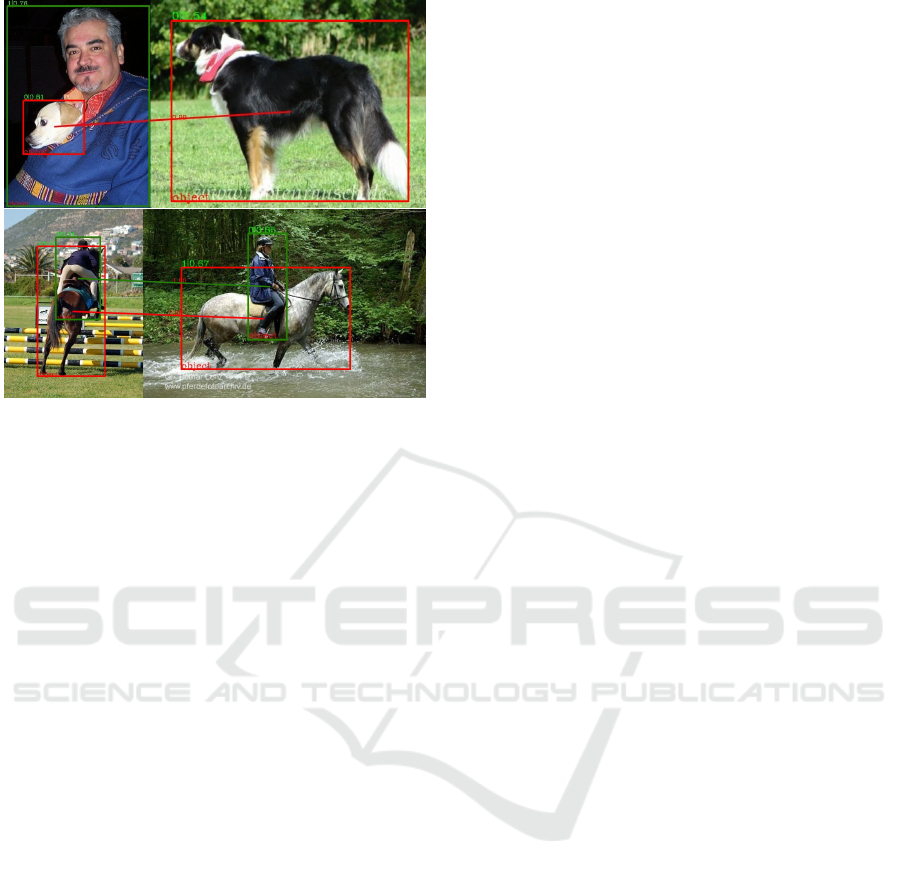
Figure 1: Illustrated results of common object detection.

adapted to any standard Single Stage Object De-

tection. Hence, the standard training pipeline can

be used, except that the classiﬁcation branch is

trained in a class-agnostic manner. This helps the

network generalize the concept of objectness seen

in training set to detect similar categories that are

unseen.

• An embedded branch is introduced to extract an

object’s representation feature, using its cosine

similarity to detect common object pairs. We in-

vestigate different loss functions for metric learn-

ing, such as classwise and pairwise losses, and

then propose a uniﬁed function named Curricu-

lum Contrastive Loss to deal with inherent prob-

lems of object detection, such as class imbalance

and small batch-size. Our proposed loss yields the

best results in our experiments.

• The model is evaluated on two dataset PASCAL

VOC 2007 and COCO 2014. Our SSCOD model

can achieve better results than the baseline of stan-

dard object detection, for both known and un-

known categories. For unknown cases, our SS-

COD can achieve comparable results with previ-

ous work.

2 LITERATURE REVIEW

2.1 Object Detection

Since the COD problem is developed based on Object

Detection framework, we review general techniques

for Object detection in this section. Object Detec-

tion framework can be separated into two main ap-

proaches, namely two stages and one stage.

Benchmarks in two-stage approach can be named

as Regional-based convolutional neural network (Gir-

shick et al., 2014), (Girshick, 2015), Faster R-CNN

(Ren et al., 2015) and Mask R-CNN (He et al., 2017).

This approach is based on a backbone CNN to ex-

tract features, which is then attached to two CNN

modules. The ﬁrst one proposes possible regions con-

taining objects, and the second module contains two

sub-nets: a classiﬁcation head to classify the object

and a regression head to predict bounding boxes off-

set from the anchor. Since Region Proposal is the core

component, recent works, such as Iterative RPN (Gi-

daris and Komodakis, 2016) or Cascade RCNN (Cai

and Vasconcelos, 2017), (Cai and Vasconcelos, 2019)

attempt to enhance its performance by adding more

stages to reﬁne the predictions. Recently, Cascade

RPN (Vu et al., 2019) improves the quality of region

proposal by using Adaptive Convolution and combine

anchor-based and anchor-free criteria to deﬁne posi-

tive boxes. (Song et al., 2020) improves the spatial

misalignment between classiﬁcation and regression

heads by using two disentangled proposals, which are

estimated by the shared proposal. In general, two-

stage approaches can achieve higher accuracy by cas-

cading more stages and reﬁne modulators. However,

it is often slower due to the framework complexity.

Single-stage detectors were developed later to im-

prove speed, and the representative works can be

named as SSD (Liu et al., 2016), YOLO (Redmon

and Farhadi, 2017), (Redmon and Farhadi, 2018),

and RetinaNet (Lin et al., 2017b). The key advan-

tage of this approach is to omit the proposal region

but use a sliding-window to produce dense predic-

tions directly. Speciﬁcally, at each cell in a feature

map, a set of default anchors with different scales

and ratios are predeﬁned. Classiﬁcation and bound-

ing box regression are then predicted directly on each

anchor. Recently, research shifts attention to re-

move the anchor-box step and propose a new kind

of framework name “anchor-box-free” approach. In

general, anchor-box-free approaches, such as FCOS

(Tian et al., 2019)), CenterNet (Duan et al., 2019),

Object-as-Points (Zhou et al., 2019), CornerNet (Law

and Deng, 2018) are designed to be simpler and more

efﬁcient. (Zhang et al., 2020) investigates the fac-

tors constituting the performance gap between anchor

and free-anchor approaches, and discover that the

main factor is how to assign positive/negative training

samples. Consequently, they propose adaptive train-

ing sample selection (ATSS) improvement to Retina

net, which surpasses all anchor and free-anchor ap-

Single Stage Class Agnostic Common Object Detection: A Simple Baseline

397

proaches without introducing any overhead. In short,

single-stage detectors currently achieve comparable

or even better accuracy than two-stages, while signif-

icantly simpler and faster.

2.2 Co-segmentation

The co-segmentation has been studied for many years

(Joulin et al., 2010), (Vicente et al., 2011) (Quan

et al., 2016), where the main goal is to segment

common foreground in the pixel level from multi-

ple images. (Yuan et al., 2017) introduced a deep

dense conditional random ﬁeld framework and used

handcrafted SIFT and HOG features to establish co-

occurrence maps. (Quan et al., 2016) proposed a

manifold ranking method that combines low-level ap-

pearance features and high-level semantic features ex-

tracted from an Imagenet pre-trained network.

However, the application of previous works is

quite restricted, since it assumes only a single com-

mon object, which also must be salient in the im-

age set. Recently, (Li et al., 2019a) proposed a deep

Siamese network to achieve object co-segmentation

from a pair of images. (Chen et al., 2019a) pro-

posed an attention mechanism to select areas that have

high activation in feature maps for all input images.

(Zhang et al., 2019) proposed a spatial-semantic mod-

ulated network, in which the spatial module roughly

locates the common foreground by capturing the cor-

relations of feature maps across images, and the se-

mantic module reﬁnes the segmentation masks. A

comprehensive review of co-segmentation methods

can be found in the recent work of (Xu et al., 2019),

(Merdassi et al., 2019). The co-segmentation setting,

however, works with pixel-level rather than object in-

stance level. Hence, the objective is different from the

COD problem.

2.3 Common Object Detection

(Bao et al., 2012) introduce a problem named object

co-detection aiming to detect if the same object is

present in a set of images. It is based on the intuition

that an object should have a consistent appearance re-

gardless of observation viewpoints. (Guo et al., 2013)

follow the principle to exploit the consistent visual

patterns from the objects. The goal then is to recog-

nize whether objects in different images correspond to

the same instance, and estimate the viewpoint trans-

formation.

Co-localization (Le et al., 2017), (Li et al., 2019b)

deﬁnes the problem as localizing categorical objects

using only a positive set of sample images. The gen-

eral approach is to utilize a classiﬁcation activation

map from a pre-trained Imagenet network to localize

the common areas. This problem is weaker since it

requires a set of positive images as input, hence the

application is limited to a single instance only.

(Jiang et al., 2019) recently extend the idea of co-

detection and co-localization and introduce common

object detection, which removes the aforementioned

limitations. In their approach, Faster-RCNN is used

as the base detector to propose foreground areas. The

object proposals are then passed to an ROI align layer

to extract object features in the second stage. Siamese

Network and Relation Matching subnet are proposed

to estimate the similarity between objects. Compared

to (Jiang et al., 2019) solution, our proposed method

is based on a Single-Stage Detector with an embedded

branch network, which is more simple and ﬂexible.

Moreover, our proposed method can achieve higher

accuracy in both seen and unseen categories, as pre-

sented in the following sections.

3 METHODOLOGY

3.1 Network Architecture

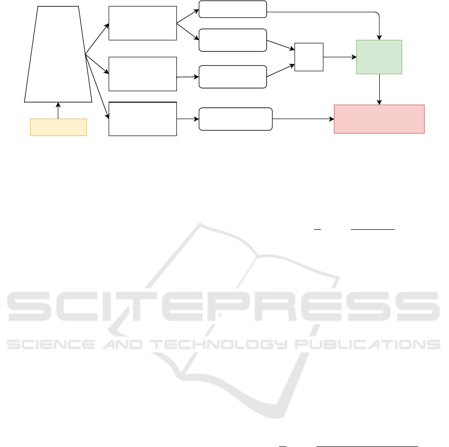
Our proposed framework, Single Stage Common Ob-

ject Detection Network (SSCOD), is illustrated in

Figure 2. The framework is built upon the standard

Single Stage Object detection, such as Retina (Lin

et al., 2017b) or FCOS (Tian et al., 2019). Specif-

ically, the network includes a Backbone to extract

features from an input image, and a Feature Pyra-

mid Network (FPN) (Lin et al., 2017a) to fuse fea-

tures from different scales. Features extracted from

P3-P7 of FPN, i.e. with resolution (H/2

,W /2

) to

(H/2

,W /2

), are passed to the detection head.

We design the SSCOD head based on the Retina

Head with ATSS (Zhang et al., 2020) sampling thanks

to its efﬁciency, although other modules such as

FCOS (Tian et al., 2019) or Centerness (Zhou et al.,

2019), (Duan et al., 2019) can be easily substituted. In

particular, the detection head has 3 branches, namely

Regression, Objectness, and Embedded Head, as il-

lustrated in Figure 2. The regression branch regresses

to bounding box location B = (x,y,w,h), and also pre-

dicts the object’s center p

, a.k.a centeredness (Zhang

et al., 2020). The objectness predicts the probability

that a bounding box contains an object. This is

similar to the classiﬁcation branch in Retina, but in

a class-agnostic manner, e.g only predict foreground

vs. background. A bounding box centering at (i, j) is

considered as a valid object if its score

s(i, j) = p

(i, j)p

(i, j) (1)

ICPRAM 2021 - 10th International Conference on Pattern Recognition Applications and Methods

398

Backbone

+FPN

RegressionHead

(4convs)

BoundingBoxB

CenternessP

ObjectnessHead

(4convs)

ObjectnessP

EmbeddedHead

(4convs)

Score

Image

Threshold,

NMS

Out:

(B(i,j),s(i,j),x(i,j))

Embedvectorx

Figure 2: Single Stage Common Object Detection Network (SSCOD).

is greater than a threshold.

To perform common class matching, we add an

embedded branch to produce a representation vector

x ∈ R

, where d is the embedded dimension and x is

normalized kxk = 1. Hence, a predicted box b

is rep-

resented by a tuple b

= (B

), and the similarity

between two predicted bounding boxes b

and b

measured by

sim(b

) = s

cos(x

) = s

(2)

Following the ATSS sampling strategy (Zhang

et al., 2020), we only use a single scale, square an-

chor, for anchor setting. To keep it simple, similar

to Retina or Mask-RCNN, each branch has 4 con-

volution layers kernel 3 × 3, although other add-on

blocks such as Deformable Conv (Zhu et al., 2019),

Nonlocal Block (Wang et al., 2018b) can be easily

added. To accommodate for small batch size, we use

Convolution with Weight Standardized (Qiao et al.,

2019) followed by a Group Normalization (GN) (Wu

and He, 2018) and a ReLu activation. Each branch

ends by a convolution layers kernel 3 × 3 without the

normalization layer. For the objectness and centered-

ness branch, the features are passed through a Sig-

moid layer.

3.2 Loss Functions

The Generalized IoU (GIoU) (Rezatoﬁghi et al.,

2019) and the Cross-Entropy losses are utilized to

train the bounding box regression and the centered-

ness branch. To train the objectness branch, we

adopt an adaptive version of Focal Loss proposed

by (Weber et al., 2019). For the embedded branch,

we consider two types of loss functions for metric

representation learning, namely class-wise and

pair-wise losses.

Class-wise losses, such as Angular Loss (Wang et al.,

2017), SphereFace (Liu et al., 2017), CosFace (Wang

et al., 2018a), ArcFace (Deng et al., 2019), use a lin-

ear layer W ∈ R

d×n

to map the embedded feature di-

mension to the number of classes n, followed by a

softmax layer:

L = −

∑

i=1

log

∑

j=1

(3)

where N is the batch size, and W

∈ R

denotes the

j-th column of W , corresponding to class y

. To en-

force feature learning, the weight W and features are

normalized, e.g. kW

k = 1 kx

k = 1, which leads to

= kW

kkx

kcos(θ

) = cos(θ

). Hence, optimiz-

ing the loss function (3) only depends on the angle

between the feature and the weight, where W

can be

associated as the center of class y

. To smoothen the

loss, the cosine value is often multiplied with a scale

s before computing softmax.

Let T (θ

) and N(θ

) be functions that modulate

the angles between positive and negative samples re-

spectively. In the simplest case (no manipulation),

T (θ

) = cos(θ

), and N(θ

) = cos(θ

), and (3) can

be rewritten as:

L = −

∑

i=1

log

sT (θ

)

sT (θ

)

∑

j=1, j6=y

sN(θ

)

(4)

Many approaches focus on modulating positive sam-

ples; for example, in ArcFace Loss, a margin m is

added to the angle of positive samples:

T (θ

) = cos(θ

+ m), N(θ

) = cos(θ

) (5)

However, negative samples are also important. In

metric representation learning, a negative sample can

be classiﬁed as: (a) hard if θ

< θ

, (b) semi-hard if

≤ θ

< θ

+ m, and (c) easy if θ

+ m ≤ θ

. Cur-

riculum Loss (Huang et al., 2020) further imposes a

Single Stage Class Agnostic Common Object Detection: A Simple Baseline

399

modulation to the negative samples:

T (θ

) = cos(θ

+ m),

N(θ

) =

(

cos(θ

) if θ

+ m ≤ θ

cos(θ

)(t + cos(θ

)) otherwise

(6)

That is, the weights of hard and semi-hard are ad-

justed during training by a modular w = t + cos(θ

Here, t is set to the average of positive cosine similar-

ity

t =

∑

cos(θ

)

. (7)

At the beginning, t ≈ 0, thus w < 1 and the effect of

hard negatives lessens, letting the model learn from

the easy negative samples ﬁrst. As the model be-

gins to converge, it can detect negative samples bet-

ter. Therefore, the number of easy negative samples

increases, i.e. θ

→ 0, hence increasing the weight t,

and switching the model’s focus from easy to the hard

negative samples.

We adopt the Curriculum Loss to compare in our

experiments. Furthermore, to deal with typical class-

imbalance problem of object detection, we also im-

pose a focal term:

L = −

∑

i=1

(1 − p

)

γ(t)

log(p

), (8)

where

sT (θ

)

sT (θ

)

∑

j=1, j6=y

sN(θ

)

(9)

Inspired by Automated Focal Loss (Weber et al.,

2019), we set γ(t) = −log(max(t,10

−5

)). In practice,

t is computed through Exponential Moving Average

of (7).

Pair-wise losses, such as Max Margin Contrastive

Loss (Hadsell et al., 2006), Triplet Loss (Weinberger

and Saul, 2009) (Schroff et al., 2015), (Hermans

et al., 2017), Multi-class N-pair loss (Sohn, 2016),

directly minimize the distances between different

samples having same classes (positive pairs) and

maximizes the distance between those of different

labels (negative pairs).

For an anchor sample x

in a data batch, we can

ﬁnd a set of positive pairs U

and negative pairs V

. Let

and N

−

as the size of U

and V

respectively, and

i j

−

i j

) be the distance between two positive (neg-

ative) samples x

and x

, where d(x

) = −x

The exact formula is d(x

) = 1 −

kkx

, but we

require kx

k = kx

k = 1 and drop constant 1 for notation

convenience since it does not affect the loss value.

for Cosine distance or d(x

) = kx

− x

for Eu-

clidean distance. When N

= 1 (or N

−

= 1 ), we

denote d

(or d

−

) as the only distance in the set. The

general form of pairwise loss is:

L =

∑

F( d

i j

j∈U

, d

−

k∈V

) (10)

In Triplet Loss (Hermans et al., 2017), for exam-

ple, F = max(0, m + max

j∈U

i j

− min

k∈V

), where m is

the margin. In Multi-class N-pair loss (Sohn, 2016),

the loss function is deﬁned as:

F = log(1 +

∑

k∈V

exp(d

− d

−

))

= −log

exp(−d

)

exp(−d

) +

∑

k∈V

exp(−d

−

)

(11)

(11) is also extended by using a temperature, as

named NT-Xent by (Chen et al., 2020), and applied

to general case where N

≥ 1, as named Supervised

Contrastive loss by (Khosla et al., 2020):

F = −

∑

j∈U

log

exp(−d

i j

/τ)

exp(−d

i j

/τ) +

∑

k6=i

exp(−d

−

/τ)

(12)

Note that, the difference between (11) and (12)

also lie in the denominator. In N-Pair loss (11), only

the negative pairs are considered ( j ∈ V

), while in

(12), all positive and negative are used (k 6= i). This is

because the NT-Xent and Supervised Contrastive loss

are originally designed for transfer learning, aiming to

learn general visual representation. In our case, since

we aim for both class intra compactness and inter sep-

arability, we also consider the negative pairs only as

in (11).

Finally, let s = 1/τ and using the Cosine distance,

(12) is rewritten as:

F = −

∑

j∈U

log

exp(scos(θ

i j

))

exp(scos(θ

i j

)) +

∑

k6=i

exp(scos(θ

))

(13)

Note that (4) and (13) share the same structure. There-

fore, we can adopt the modulation deﬁned in (5) or (6)

to rewrite (13) as:

F = −

∑

j∈U

log

sT (θ

i j

)

sT (θ

i j

)

∑

k∈V

sN(θ

)

(14)

We name the former combination as Arc Con-

trastive (ArcCon) loss and the later as Curriculum

Contrastive (CurCon) loss. For CurCon Loss, we

compute t =

∑

i=1

min

j∈U

(cosθ

i j

). Table 1 summarizes

the loss functions proposed in this paper.

ICPRAM 2021 - 10th International Conference on Pattern Recognition Applications and Methods

400

Table 1: Summary of Loss Functions for embedded matching.

Loss

Focal Curriculum

(FocalCur)

Arc Contrastive

(ArcCon)

Arc Contrastive -Negative

(ArcCon-Neg)

Curriculum Contrastive

(CurCon)

Formular Equ. (8) (14), k 6= i as in (13) (14), k ∈ V

as in (11) (14), k 6= i as in (13)

T (θ),N(θ) (6) (5) (5) (6)

4 EXPERIMENTS

4.1 Experimental Setup

Our experiments are conducted on the popular PAS-

CAL VOC (Everingham et al., 2010) and the large-

scale detection benchmarks COCO 2014 (Lin et al.,

2014). Following the common practice (Zhang et al.,

2018), (Zoph et al., 2019), (Zhang et al., 2019), we

use both the trainval VOC 2007 and VOC 2012 for

training (21.5k images and replicate 3 times), and

evaluate on VOC2007 (5K images) test set. For the

COCO dataset, we use the trainval35k split (115K im-

ages) for training and report the results on the minival

split (5K images). Our code is implemented based on

MMDetection opensource (Chen et al., 2019b).

Training Details. We conduct the experiments using

the standard setup with backbone Resnet50 (R50) pre-

trained from ImageNet. The stem convolution, the

ﬁrst stage, and Batch Norm layers of backbone R50

are frozen. For FPN and Head, we use Weight Stan-

dardized Convolution (Qiao et al., 2019) and Group

Norm (Wu and He, 2018). The model is trained with

stochastic gradient descent (SGD) with momentum

0.9 and weight decay 10

−4

, with batch sizes (BS)

equal 16. We train the models with 12 epochs for

both VOC and COCO datasets.

We evaluate the effectiveness of both class-wise

losses and pair-wise losses presented in Section. 3.2.

If a pair-wise loss is used, for each image in the batch,

we also randomly sample another image that has at

least one common object to form a valid pair. Hence

the number of images in the batch is doubled. There-

fore, we reduce the batch size a haft to make con-

sistent training setting, but still keep the notation of

batch size unchanged. In addition, we use auto policy

V0 (Zoph et al., 2019) for data augmentation. For the

VOC dataset, the shorter side of the input images is

resized to 600 pixels, while ensuring the longer side

is smaller than 1000 pixels, and the aspect ratio is

kept unchanged. In short, we denote it as resize to

(1000,600). For the COCO dataset, the images are

set to a size of (1333,800). All images after resizing

are padded to be divisible by 32.

We investigate different losses presented in Table

1. To ﬁnd appropriate parameters for the loss func-

tions, we ﬁrst train and evaluate the model on the val-

idation set of VOC2007. We observe that ArcFace

and CurricularFace are sensitive to parameter s, and

s = 4,m = 0.5 yields the best result. For pair-wise

losses, s ∈ [1,4], m = 0.5 yields quite equivalent re-

sults, and select s = 1,m = 0.5 as the default value for

our experiments.

Inference and Evaluation Details. We ﬁrst forward

the input image through the network and obtain the

predicted bounding boxes with a conﬁdence score

and embedded feature vector. We use the same post-

processing parameters with RetinaNet (threshold 0.05

and NMS with maximum of 100 bounding boxes per

image). For inference, two bounding boxes are con-

sidered belonging to a common class if their similar-

ity score is greater than a threshold.

For evaluation, we extract the top 100 pairs that

have the highest matching scores from all possible

matching pairs of two images. We evaluate the model

using both Recall and Average Precision (AP) with

the VOC evaluation style. Speciﬁcally, among the

top 100 pairs, a predicted pair is true positive if it

satisﬁes both conditions: (a) Each bounding box

has IoU > 0.5 with ground-truth boxes. (b) Their

ground-truth boxes have the same object categories.

Otherwise, it is a false positive. To generate ground

truth, although arbitrary number of pairs can be

used, we follow (Jiang et al., 2019) to randomly

sample p = 6 valid pairs for each image in the

validation dataset, where the random seed is set to 0

for reproducibility.

Baseline Model. The easiest solution for common

object detection is to use the standard object detection

approach, then a common pair can be estimated by:

• Hard matching (HM): Object category of each

bounding box can be inferred as the class having

the highest probability. Two bounding boxes form

a valid pair if they predict the same class.

• Soft matching (SM): The probability score is used

as a description vector, and matching score can be

computed as their cosine similarity. The inference

hence follows the same setup of our solution.

Single Stage Class Agnostic Common Object Detection: A Simple Baseline

401

4.2 Pascal VOC

The learning rate is linearly increased using warm-up

strategy to 0.5e

−2

in the ﬁrst 300 iterations, and then

gradually reduced by the cosine annealing to 0.5e

−4

Experiment Type 1. First, to verify if our SSCOD

degrades the accuracy for known categories, we train

the standard model ATSS with R50 backbone by com-

mon setting, and infer the Hard-matching (HM) and

Soft-Matching (SM) baseline. In this experiment,

our baseline model without test-time augmentation

or complex structure achieves 0.774 mAP, which is

similar or higher than several benchmark results (Ren

et al., 2015), (Liu et al., 2016) (Fu et al., 2017). This

validates that our model can be a strong baseline.

Similarly, we train the proposed SSCOD model with

different losses. The experiments are conducted using

all samples of 20 classes, and the result is presented

in Table 2.

As seen from Table 2, results of SSCOD are

asymptotic to those of the baseline. Speciﬁcally,

SSCOD trained with FocalCur loss achieves 0.5986

AP, which is closely matched to the HM baseline of

0.6052 AP and higher than SM baseline of 0.5746 AP.

The CurCon loss obtains the best result in this case,

which is 0.6141AP and higher than both baselines.

The ArcCon loss yields slightly worse result than the

HM baseline, but still better than SM baseline.

Note that, images in VOC dataset often has

only one or two classes. Hence, the performance

of baseline for VOC is quite predictable from its

mAP, since the precision when predicting a pair is

conditional on the precision of each box component,

e.g. mAP

= 0.774

≈ 0.6. The hard matching yields

higher accuracy than soft-matching because it can

suppress the noise better through the post processing.

Nevertheless, our SSCOD using cosine similarity can

achieve comparable or better results. Surprisingly,

ArcCon-Neg yields the worst result. This is possibly

due to insufﬁcient number of negative pairs, which

is even more severe due to small batch size used in

object detection.

Experiment Type 2. Second, to evaluate the ability to

detect common pairs of unseen categories, we remove

the ﬁve classes from the training set. For simplic-

ity and reproducibility, we chose the last ﬁve classes,

namely: potted plant, sheep, sofa, train and tv mon-

itor, and repeat similar experiments on the truncated

training set. Different from the known-category case,

the unseen case depends on both the localization abil-

ity of the objectness branch and the matching accu-

racy of embedded features. Hence, to independently

evaluate the matching module, we train the object-

ness branch using all samples from the dataset. We

emphasize that this is solely to learn foreground and

background concept, hence no object category infor-

mation is used. Follow (Jiang et al., 2019), we denote

unseen classes as Only Novel Categories (ONC) and

seen classes as Excluded ONC (EONC), and the ex-

periment results are shown in Table 3.

As seen from Table 3, although the baseline

model yields the highest results for EONC test,

it can’t detect novel classes in ONC test. This is

expected due the standard object detection is only

designed for close-set condition. In contrast, our

SSCOD is still able to match objects from unseen

classes. Speciﬁcally, ArcCon loss yields the best

result for ONC test, 0.2765AP. On the other hand,

CurCon loss gets a better balance between EONC

and ONC tests, 0.5857AP, and 0.2663AP for objects

of seen and unseen categories respectively. Focal-

Cur loss yields worse results for ONC test in this case.

Experiment Type 3. Finally, we evaluate the models

in the most restricted case, where both objectness and

embedded branches are trained with samples from

only 15 seen classes. In practice, since one image may

contain several objects, simply dropping samples of

unknown classes will force the network treating them

as background, thus harm the network generalization.

To overcome this problem, we simply set the weight

for samples of unknown classes equal 0 during com-

puting the loss for objectness branch and regression

branches. Note that, this setting does not restrict real

application because in practice all samples are used

to train the network, and unlabeled objects are often

not interesting. For the embedded branch, these sam-

ples are totally ignored. The highest results of each

experiment are presented in Table 4.

As seen from Table 4, ArcCon and CurCon per-

form best in this case, while FocalCur and ArcCon-

Neg perform worst. The CurCon loss still yields the

best balance between EONC and ONC test, 0.5593AP

and 0.1212AP for seen and unseen categories respec-

tively. However, different from previous experiments,

we observe the trade-off between EONC and ONC’s

performance.

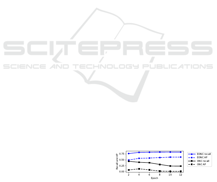
Figure 3: Trade-Off between EONC and ONC test in Ex-

periment Type 3 using CurCon Loss.

ICPRAM 2021 - 10th International Conference on Pattern Recognition Applications and Methods

402

Table 2: Comparison between the baseline model and SSCOD model for Experiment Type 1 on VOC dataset . Bold and Both

Italic represent the best results of baseline and SSCOD, respectively.

Eval.

Metrics

Baseline SSCOD

HM SM FocalCur ArcCon ArcCon-Neg CurCon

Recall 0.7922 0.7976 0.7208 0.7771 0.6356 0.8090

AP 0.6052 0.5746 0.5986 0.5832 0.5326 0.6141

Table 3: Comparison between the baseline model and SSCOD model for Experiment Type 2 on the VOC dataset. Bold and

Both Italic represent the best results of baseline and SSCOD, respectively.

Type

Eval.

Metrics

Baseline SSCOD

HM SM FocalCur ArcCon ArcCon-Neg CurCon

EONC

Recall 0.8128 0.8123 0.8078 0.8232 0.7752 0.8385

AP 0.6278 0.6001 0.5443 0.5505 0.4798 0.5857

ONC

Recall 0.0699 0.0850 0.5925 0.6211 0.5936 0.6267

AP 0.0012 0.0014 0.1906 0.2765 0.2510 0.2663

Table 4: Comparison between the baseline model and SSCOD model for Experiment Type 3 on the VOC dataset. Bold and

Both Italic represent the best results of baseline and SSCOD, respectively.

Type

Eval.

Metrics

Baseline SSCOD

HM SM FocalCur ArcCon ArcCon-Neg CurCon

EONC

Recall 0.8128 0.8123 0.7347 0.7509 0.4103 0.8105

AP 0.6278 0.6001 0.4262 0.4595 0.2572 0.5593

ONC

Recall 0.0699 0.0850 0.3563 0.4060 0.3418 0.3810

AP 0.0012 0.0014 0.066 0.1391 0.0567 0.1212

As illustrated in Fig. 3, the longer training, the

better EONC test but the worse ONC test. This is be-

cause the objectness and regression branches start to

overﬁt to the seen classes, hence decrease the local-

ization ability for unseen classes. This effect does not

happen in Type 2 experiments.

4.3 COCO 2014

We conduct similar experiments on the COCO dataset

for type 1 and 2 as done in VOC.

Experiment Type 1. The learning rate is linearly in-

creased using warm-up strategy to 1e

−2

in the ﬁrst

500 iterations, and then gradually reduced by the co-

sine annealing to 1e

−4

. Since ArcCur-Neg loss does

not yield comparable results with other, we exclude it

for COCO experiments. For the baseline, we use the

checkpoint

provided by MMDetection, which has

39.4 box mAP.

The results are shown in Table 5. In this case, Cur-

Con loss yields the best performance and surpasses

the base-line with a large margin for both recall and

AP, 0.5862 and 0.3811 respectively. FocalCur loss

also yields closely matching results with the baseline.

These results are consistent with VOC’s results, hence

conﬁrm the effectiveness of our proposed approach.

https://github.com/open-

mmlab/mmdetection/tree/master/conﬁgs/atss

Experiment Type 2. Unlike VOC, COCO dataset

has many ﬁne-granded classes in each meta-classes,

namely: person, vehicle, outdoor, animal, accessory,

sports, kitchen, food, furniture, electronics, appli-

ance, and indoor. Therefore, selecting seen and un-

seen categories for training and evaluation can have

a signiﬁcant effect on the AP score. For example, if

both car and bus are in unseen classes, their high score

matching is reasonable but false-positive. Therefore,

we conduct two experiments:

• Case A: Follow (Jiang et al., 2019), we select 30

classes to train the model. However, since they do

not specify the class names, reproducing is hard.

Here, we choose the training classes as: person,

bicycle, car, airplane, boat, ﬁre hydrant, stop sign,

dog, horse, elephant, umbrella, handbag, snow-

board, sports ball, baseball bat, skateboard, bot-

tle, fork, bowl, apple, carrot, cake, chair, toilet,

laptop, cell phone, microwave, sink, book, and

hair drier.

• Case B: We split 75% classes for training, and

25% other for testing. Concretely, 20 unseen

classes are: motorcycle, bus, cat, horse, sheep,

backpack, tie, skis, sports ball, surfboard, tennis

racket, cup, banana, hot dog, pizza, donuts, re-

mote, toaster, clock, teddy bear.

We report the results using only CurCon loss in Ta-

ble 6, since we found it yields the best results in all

Single Stage Class Agnostic Common Object Detection: A Simple Baseline

403

Table 5: Comparison between the baseline model and SSCOD model for Experiment Type 1 on the COCO dataset. Bold and

Both Italic represent the best results of baseline and SSCOD, respectively.

Eval

Metrics

Baseline SSCOD

HM SM FocalCur ArcCur CurCon

Recall 0.5128 0.5102 0.5101 0.5473 0.5862

AP 0.3688 0.3515 0.3615 0.3160 0.3811

Table 6: Comparison between the baseline model and SSCOD model for Experiment Type 2 on the COCO dataset. Bold and

Both Italic represent the best results of baseline and SSCOD, respectively.

Type

Eval

Metrics

Case A Case B

Baseline SSCOD Baseline SSCOD

Metrics HM SM CurCon HM SM CurCon

EONC

Recall 0.5141 0.5075 0.5862 0.5247 0.5206 0.6201

AP 0.3676 0.3501 0.3811 0.3781 0.3603 0.4074

ONC

Recall 0.0545 0.0595 0.4202 0.0739 0.0540 0.4587

AP 0.0003 0.0003 0.0643 0.0003 0.0003 0.1213

previous experiments. For EONC test, SSCOD yields

higher results than the baseline with a large margin,

0.3811AP and 0.4074AP for case A and B respec-

tively. As previously mentioned, the baseline can not

work for ONC test. For Case A, the performance is

poor due to the shortage of training samples. For Case

B, the results are better, e.g. 0.1213AP, due to a larger

number of training samples.

4.4 Discussion

4.4.1 Comparison of Loss Functions

Although the class-wise and pairwise losses have

been used for Face-ID or unsupervised learning, this

work adopts them for (unseen) object detection. In

our experiments, the pairwise losses are more effec-

tive than the classwise loss. We hypothesize that this

is because in classwise loss, the number of contrastive

pairs in the denominator is limited to the number of

known classes (the centroid of each class) from the

train set. In contrast, the number of pairs in the de-

nominator of pairwise losses is essentially all possi-

ble object pair combinations, governed by the num-

ber of bounding boxes in a minibatch. This helps in-

crease the interaction between the sample pairs, and

especially useful for the case of unknown classes de-

tection. Our results are in-line with recent research

of contrastive learning (Chen et al., 2020) (He et al.,

2020), who also ﬁnds the importance of using a large

training batch size to increase the number of negative

pairs for good performance.

Our proposed Curriculum Contrastive Loss per-

forms best in most of experiments, since it uniﬁes

both approaches by adding the adaptive angular mar-

gins to the contrastive loss formulation.

4.4.2 Comparison to Previous Works

To compare with previous works, we attempt to re-

produce the results of (Jiang et al., 2019). How-

ever, this is challenging, due to missing information.

Speciﬁcally, in our reproducing attempt, their pro-

posed Siamese Network was unstable during train-

ing, e.g. when sim(p

, p

) < 0 in their Equ (7), the

loss is NaN. Also for the Siamese network, sampling

strategy is critical for convergence but unmentioned.

Similarly, in their proposed Relation Matching net-

work, concat( f

, f

) and concat( f

, f

) can yield dif-

ferent results. Furthermore, missing information such

as how to select 20 images pair for training, how

to select seen/unseen classes, and setup optimization

makes the reproducing process very difﬁcult. Hence,

we use their reported results for direct comparison,

albeit possibly different settings.

As seen from Tab. 7 and Tab. 8, their EONC re-

sults are always worse then the baseline, while ONC

is better. This is questionable, since the model is

trained on seen classes, it should perform better for

EONC case. This is contrast with our results. In

the Type 1 experiments, our SSCOD always performs

better the baseline, which also has much higher AP

than the Faster-RCNN baseline used by (Jiang et al.,

2019). This conﬁrms the effectiveness of our pro-

posed methods.

For ONC test, our results on VOC is still higher

than the Siamese and Relation Network methods re-

ported by (Jiang et al., 2019). In addition, our pro-

posed approach does not require complicated training

setup, ofﬂine sampling mechanism or extra matching

modulation, therefore can serve as a good baseline.

In contrast, our proposed method perform worse on

COCO dataset, which is likely due to missing detec-

tion for unknown objects.

However, there are still ample room to improve

ICPRAM 2021 - 10th International Conference on Pattern Recognition Applications and Methods

404

Table 7: Comparison between the proposed method and previous works on the VOC dataset. Bold represents the best results.

Type

Ours Jiang et al. 2019

FocalCur ArcCon ArcCon-Neg CurCon Best Baseline Siamese Relation

EONC 0.5443 0.5505 0.4798 0.5857 0.4481 0.3269 0.3774

ONC 0.1906 0.2765 0.251 0.2663 0.1638 0.2187 0.2535

Table 8: Comparison between the proposed method and previous works on the COCO dataset. Bold represents the best

results.

Type

Ours Jiang et al. 2019

CurCon Best Baseline Siamese Relation

EONC 0.3811 0.2107 0.141 0.1773

ONC 0.0643 0.1247 0.1398 0.1824

the results. As showed in Tab. 4 and Fig. 3, the

network can be easily trained to optimize the perfor-

mance on seen classes, but this will reduce the ability

to generalize for unseen objects. This problem can

be partially alleviated by training on larger and more

diverse dataset. In addition, we can also treat it as

positive-unlabeled problem (Yang et al., 2020) to re-

duce the effect of missing labels. Currently, the ob-

jectness, the regression and the embedded branches

are trained independently, and this can be insufﬁcient.

Adding an attention mechanism from embedded fea-

tures to the objectness can also enhance the results.

We leave the discussion above for future work.

4.4.3 Result Visualization

Due to space limitations, visualization of predicted re-

sults and the pretrained model to generate predictions

can be found at (URL).

5 CONCLUSION

This paper proposes a solution for common object de-

tection, which aims to detect pairs of objects from

similar categories in a set of images. While this is an

interesting problem, there are many challenges, such

as the ability to work on both closed-set and open-set

conditions, and for multiple objects. Our solution is

built upon single-stage object detection thanks to its

efﬁciency. To matching objects of the same category,

we add an embedded branch to the network to gener-

ate representation features. Several loss functions to

train the embedded branch are investigated. The pro-

posed Curriculum Contrastive loss, which combines

contrastive learning and angular margin losses, gives

the best performance. The experiments on both VOC

and COCO dataset demonstrate that our approach

yields higher accuracy than the base-line of standard

object detection for both seen and unseen categories.

We hope this work can serve as a strong baseline for

future research of Common Object Detection.

REFERENCES

Bao, S. Y., Xiang, Y., and Savarese, S. (2012). Object co-

detection. Lecture Notes in Computer Science, 7572

LNCS(PART 1):86–101.

Cai, Z. and Vasconcelos, N. (2017). Cascade R-CNN: Delv-

ing into High Quality Object Detection. Proceedings

of the IEEE Computer Society Conference on Com-

puter Vision and Pattern Recognition, pages 6154–

6162.

Cai, Z. and Vasconcelos, N. (2019). Cascade r-cnn: high

quality object detection and instance segmentation.

IEEE Transactions on Pattern Analysis and Machine

Intelligence.

Chen, H., Huang, Y., and Nakayama, H. (2019a). Se-

mantic Aware Attention Based Deep Object Co-

segmentation. Lecture Notes in Computer Science,

11364 LNCS:435–450.

Chen, K., Wang, J., Pang, J., Cao, Y., Xiong, Y., Li, X.,

Sun, S., Feng, W., Liu, Z., Xu, J., Zhang, Z., Cheng,

D., Zhu, C., Cheng, T., Zhao, Q., Li, B., Lu, X., Zhu,

R., Wu, Y., Dai, J., Wang, J., Shi, J., Ouyang, W.,

Loy, C. C., and Lin, D. (2019b). MMDetection: Open

MMLab Detection Toolbox and Benchmark. arXiv

preprint arXiv:1906.07155.

Chen, T., Kornblith, S., Norouzi, M., and Hinton, G.

(2020). A Simple Framework for Contrastive

Learning of Visual Representations. arXiv preprint

arXiv:2002.05709.

Deng, J., Guo, J., Xue, N., and Zafeiriou, S. (2019). Ar-

cFace: Additive angular margin loss for deep face

recognition. Proceedings of the IEEE Computer So-

ciety Conference on Computer Vision and Pattern

Recognition, 2019-June:4685–4694.

Duan, K., Bai, S., Xie, L., Qi, H., Huang, Q., and Tian, Q.

(2019). Centernet: Keypoint triplets for object detec-

tion. In Proceedings of the IEEE International Con-

ference on Computer Vision, pages 6569–6578.

Everingham, M., Van Gool, L., Williams, C. K., Winn, J.,

and Zisserman, A. (2010). The pascal visual object

Single Stage Class Agnostic Common Object Detection: A Simple Baseline

405

classes (VOC) challenge. International Journal of

Computer Vision, 88(2):303–338.

Fu, C.-y., Liu, W., Ranga, A., Tyagi, A., and Berg, A. C.

(2017). DSSD : Deconvolutional Single Shot Detec-

tor. arXiv preprint arXiv:1701.06659.

Gidaris, S. and Komodakis, N. (2016). Attend Reﬁne

Repeat : Active Box Proposal. arXiv preprint

arXiv:1606.04446v1.

Girshick, R. (2015). Fast r-cnn. In Proceedings of the IEEE

international conference on computer vision, pages

1440–1448.

Girshick, R., Donahue, J., Darrell, T., and Malik, J. (2014).

Rich feature hierarchies for accurate object detection

and semantic segmentation. Proceedings of the IEEE

Computer Society Conference on Computer Vision

and Pattern Recognition, pages 580–587.

Guo, X., Liu, D., Jou, B., Zhu, M., Cai, A., and Chang, S. F.

(2013). Robust object co-detection. Proceedings of

the IEEE Computer Society Conference on Computer

Vision and Pattern Recognition, pages 3206–3213.

Hadsell, R., Chopra, S., and LeCun, Y. (2006). Dimension-

ality reduction by learning an invariant mapping. Pro-

ceedings of the IEEE Computer Society Conference

on Computer Vision and Pattern Recognition, 2:1735–

1742.

He, K., Fan, H., Wu, Y., Xie, S., and Girshick, R. (2020).

Momentum contrast for unsupervised visual represen-

tation learning. In Proceedings of the IEEE/CVF Con-

ference on Computer Vision and Pattern Recognition,

pages 9729–9738.

He, K., Gkioxari, G., Dollar, P., and Girshick, R. (2017).

Mask R-CNN. Proceedings of the IEEE International

Conference on Computer Vision, 2017-Octob:2980–

2988.

Hermans, A., Beyer, L., and Leibe, B. (2017). In Defense

of the Triplet Loss for Person Re-Identiﬁcation. arXiv

preprint arXiv:1703.07737.

Huang, Y., Wang, Y., Tai, Y., Liu, X., Shen, P., Li, S., Li, J.,

and Huang, F. (2020). Curricularface: adaptive cur-

riculum learning loss for deep face recognition. In

Proceedings of the IEEE/CVF Conference on Com-

puter Vision and Pattern Recognition, pages 5901–

5910.

Jiang, S., Liang, S., Chen, C., Zhu, Y., and Li, X. (2019).

Class Agnostic Image Common Object Detection.

IEEE Transactions on Image Processing, 28(6):2836–

2846.

Joulin, A., Bach, F., and Ponce, J. (2010). Discriminative

clustering for image co-segmentation. Proceedings of

the IEEE Computer Society Conference on Computer

Vision and Pattern Recognition, pages 1943–1950.

Khosla, P., Teterwak, P., Wang, C., Sarna, A., Tian, Y.,

Isola, P., Maschinot, A., Liu, C., and Krishnan, D.

(2020). Supervised Contrastive Learning. arXiv

preprint arXiv:2004.11362, pages 1–18.

Law, H. and Deng, J. (2018). Cornernet: Detecting objects

as paired keypoints. Lecture Notes in Computer Sci-

ence, 11218 LNCS:765–781.

Le, H., Yu, C. P., Zelinsky, G., and Samaras, D. (2017). Co-

localization with Category-Consistent Features and

Geodesic Distance Propagation. Proceedings - 2017

IEEE International Conference on Computer Vision

Workshops, ICCVW 2017, 2018-Janua:1103–1112.

Li, W., Hosseini Jafari, O., and Rother, C. (2019a). Deep

Object Co-segmentation. In Lecture Notes in Com-

puter Science, volume 11363 LNCS, pages 638–653.

Li, W., Jafari, H., and Rother, C. (2019b). Localizing Com-

mon Objects Using Common Component Activation

Map. pages 28–31.

Lin, T.-Y., Doll

ar, P., Girshick, R., He, K., Hariharan, B.,

and Belongie, S. (2017a). Feature pyramid networks

for object detection. In Proceedings of the IEEE con-

ference on computer vision and pattern recognition,

pages 2117–2125.

Lin, T. Y., Goyal, P., Girshick, R., He, K., and Dollar,

P. (2017b). Focal Loss for Dense Object Detection.

IEEE Transactions on Pattern Analysis and Machine

Intelligence, 42(2):318–327.

Lin, T. Y., Maire, M., Belongie, S., Hays, J., Perona, P., Ra-

manan, D., Doll

ar, P., and Zitnick, C. L. (2014). Mi-

crosoft COCO: Common objects in context. In Lec-

ture Notes in Computer Science, volume 8693 LNCS,

pages 740–755.

Liu, W., Anguelov, D., Erhan, D., Szegedy, C., Reed, S.,

Fu, C. Y., and Berg, A. C. (2016). SSD: Single shot

multibox detector. Lecture Notes in Computer Sci-

ence, 9905 LNCS:21–37.

Liu, W., Wen, Y., Yu, Z., Li, M., Raj, B., and Song, L.

(2017). SphereFace: Deep hypersphere embedding

for face recognition. Proceedings - 30th IEEE Con-

ference on Computer Vision and Pattern Recognition,

CVPR 2017, 2017-Janua:6738–6746.

Merdassi, H., Barhoumi, W., and Zagrouba, E. (2019). A

Comprehensive Overview of Relevant Methods of Im-

age Cosegmentation. Expert Systems with Applica-

tions, 140:112901.

Qiao, S., Wang, H., Liu, C., Shen, W., and Yuille, A.

(2019). Weight Standardization. arXiv preprint

arXiv:1903.10520.

Quan, R., Han, J., Zhang, D., and Nie, F. (2016). Object

Co-segmentation via Graph Optimized-Flexible Man-

ifold Ranking. In 2016 IEEE Conference on Com-

puter Vision and Pattern Recognition (CVPR), pages

687–695.

Redmon, J. and Farhadi, A. (2017). YOLO9000: Better,

faster, stronger. Proceedings - 30th IEEE Conference

on Computer Vision and Pattern Recognition, CVPR

2017, 2017-Janua:6517–6525.

Redmon, J. and Farhadi, A. (2018). YOLOv3:

An Incremental Improvement. arXiv preprint

arXiv:1804.02767.

Ren, S., He, K., Girshick, R., and Sun, J. (2015). Faster

r-cnn: Towards real-time object detection with region

proposal networks. In Advances in neural information

processing systems, pages 91–99.

Rezatoﬁghi, H., Tsoi, N., Gwak, J., Sadeghian, A., Reid,

I., and Savarese, S. (2019). Generalized intersection

over union: A metric and a loss for bounding box re-

gression. In Proceedings of the IEEE Conference on

ICPRAM 2021 - 10th International Conference on Pattern Recognition Applications and Methods

406

Computer Vision and Pattern Recognition, pages 658–

666.

Schroff, F., Kalenichenko, D., and Philbin, J. (2015).

FaceNet: A uniﬁed embedding for face recognition

and clustering. Proceedings of the IEEE Computer

Society Conference on Computer Vision and Pattern

Recognition, 07-12-June:815–823.

Sohn, K. (2016). Improved deep metric learning with multi-

class N-pair loss objective. Advances in Neural Infor-

mation Processing Systems, (Nips):1857–1865.

Song, G., Liu, Y., and Wang, X. (2020). Revisiting the sib-

ling head in object detector. In Proceedings of the

IEEE/CVF Conference on Computer Vision and Pat-

tern Recognition, pages 11563–11572.

Tian, Z., Shen, C., Chen, H., and He, T. (2019). Fcos: Fully

convolutional one-stage object detection. In Proceed-

ings of the IEEE international conference on com-

puter vision, pages 9627–9636.

Vicente, S., Rother, C., and Kolmogorov, V. (2011). Object

cosegmentation. Proceedings of the IEEE Computer

Society Conference on Computer Vision and Pattern

Recognition, pages 2217–2224.

Vu, T., Jang, H., Pham, T. X., and Yoo, C. (2019). Cas-

cade rpn: Delving into high-quality region proposal

network with adaptive convolution. In Advances in

Neural Information Processing Systems, pages 1432–

1442.

Wang, H., Wang, Y., Zhou, Z., Ji, X., Gong, D., Zhou, J., Li,

Z., and Liu, W. (2018a). CosFace: Large Margin Co-

sine Loss for Deep Face Recognition. Proceedings of

the IEEE Computer Society Conference on Computer

Vision and Pattern Recognition, pages 5265–5274.

Wang, J., Zhou, F., Wen, S., Liu, X., and Lin, Y. (2017).

Deep Metric Learning with Angular Loss. Proceed-

ings of the IEEE International Conference on Com-

puter Vision, 2017-Octob:2612–2620.

Wang, X., Girshick, R., Gupta, A., and He, K. (2018b).

Non-local neural networks. In Proceedings of the

IEEE conference on computer vision and pattern

recognition, pages 7794–7803.

Weber, M., F

urst, M., and Z

ollner, J. M. (2019). Automated

Focal Loss for Image based Object Detection. arXiv

preprint arXiv:1904.09048.

Weinberger, K. Q. and Saul, L. K. (2009). Distance metric

learning for large margin nearest neighbor classiﬁca-

tion. Journal of Machine Learning Research, 10:207–

244.

Wu, Y. and He, K. (2018). Group normalization. In Pro-

ceedings of the European Conference on Computer Vi-

sion (ECCV), pages 3–19.

Xu, H., Lin, G., and Wang, M. (2019). A Review of

Recent Advances in Image Co-Segmentation Tech-

niques. IEEE Access, 7:182089–182112.

Yang, Y., Liang, K. J., and Carin, L. (2020). Object Detec-

tion as a Positive-Unlabeled Problem. arXiv preprint

arXiv:2002.04672.

Yuan, Z., Lu, T., and Wu, Y. (2017). Deep-dense condi-

tional random ﬁelds for object co-segmentation. IJ-

CAI International Joint Conference on Artiﬁcial Intel-

ligence, pages 3371–3377.

Zhang, S., Chi, C., Yao, Y., Lei, Z., and Li, S. Z. (2020).

Bridging the gap between anchor-based and anchor-

free detection via adaptive training sample selection.

In Proceedings of the IEEE/CVF Conference on Com-

puter Vision and Pattern Recognition, pages 9759–

9768.

Zhang, S., Wen, L., Bian, X., Lei, Z., and Li, S. Z. (2018).

Single-shot reﬁnement neural network for object de-

tection. In Proceedings of the IEEE conference on

computer vision and pattern recognition, pages 4203–

4212.

Zhang, Z., He, T., Zhang, H., Zhang, Z., Xie, J., and Li, M.

(2019). Bag of Freebies for Training Object Detection

Neural Networks. arXiv preprint arXiv:1902.04103.

Zhou, X., Wang, D., and Kr

ahenb

uhl, P. (2019). Objects as

Points. arXiv preprint arXiv:1904.07850.

Zhu, X., Hu, H., Lin, S., and Dai, J. (2019). Deformable

convnets v2: More deformable, better results. In Pro-

ceedings of the IEEE Conference on Computer Vision

and Pattern Recognition, pages 9308–9316.

Zoph, B., Cubuk, E. D., Ghiasi, G., Lin, T.-Y., Shlens,

J., and Le, Q. V. (2019). Learning Data Augmenta-

tion Strategies for Object Detection. arXiv preprint

arXiv:1906.11172.

Single Stage Class Agnostic Common Object Detection: A Simple Baseline

407