
Advancing Eosinophilic Esophagitis Diagnosis and Phenotype
Assessment with Deep Learning Computer Vision
William Adorno III
1
, Alexis Catalano
2,3
, Lubaina Ehsan
3
, Hans Vitzhum von Eckstaedt
3
,
Barrett Barnes
4
, Emily McGowan
5
, Sana Syed
4,∗
and Donald E. Brown
6,∗
1
Dept. of Engineering Systems and Environment, University of Virginia, Charlottesville, VA, U.S.A.
2
College of Dental Medicine, Columbia University, New York City, NY, U.S.A.
3
School of Medicine, University of Virginia, Charlottesville, VA, U.S.A.
4
Department of Pediatrics, School of Medicine, University of Virginia, Charlottesville, VA, U.S.A.
5
Department of Medicine, University of Virginia, Charlottesville, VA, U.S.A.
6
School of Data Science, University of Virginia, Charlottesville, VA, U.S.A.
Keywords:
Image Segmentation, Eosinophilic Esophagitis, Eosinophils, U-Net, Convolutional Neural Networks.
Abstract:
Eosinophilic Esophagitis (EoE) is an inflammatory esophageal disease which is increasing in prevalence. The
diagnostic gold-standard involves manual review of a patient’s biopsy tissue sample by a clinical pathologist
for the presence of 15 or greater eosinophils within a single high-power field (400× magnification). Diag-
nosing EoE can be a cumbersome process with added difficulty for assessing the severity and progression of
disease. We propose an automated approach for quantifying eosinophils using deep image segmentation. A
U-Net model and post-processing system are applied to generate eosinophil-based statistics that can diagnose
EoE as well as describe disease severity and progression. These statistics are captured in biopsies at the initial
EoE diagnosis and are then compared with patient metadata: clinical and treatment phenotypes. The goal is to
find linkages that could potentially guide treatment plans for new patients at their initial disease diagnosis. A
deep image classification model is further applied to discover features other than eosinophils that can be used
to diagnose EoE. This is the first study to utilize a deep learning computer vision approach for EoE diagnosis
and to provide an automated process for tracking disease severity and progression.
1 INTRODUCTION
Eosinophilic Esophagitis (EoE) is a chronic aller-
gen/immune disease that occurs when eosinophils,
a type white blood cell, concentrate in the esopha-
gus. It occurs in roughly 0.5 - 1.0 in 1,000 people
and is found in 2 - 7% of patients who undergo en-
doscopy for any reason (Dellon, 2014). EoE is be-
lieved to be triggered by dietary components in pa-
tients and is increasing in prevalence (Carr et al.,
2018). Clinical symptoms include swallowing diffi-
culties, food impaction, and chest pain (Runge et al.,
2017). Persistent esophageal inflammation can even-
tually progress to strictures in the esophagus with the
need for interventional procedures such as dilations,
which can significantly impact the quality of patients’
lives. The most characteristic microscopic patho-
logic feature used to diagnose EoE is intraepithelial
eosinophil inflammation. For diagnosis, patients with
clinical symptoms concerning for EoE undergo an
endoscopy and the collected biopsy tissue samples
are then evaluated for presence of eosinophils. The
accepted criterion for pathologists to diagnose EoE
involves identifying at least one High-Power Field
(HPF; 400× magnification adjustment) within a pa-
tient’s tissue biopsy slide that contains 15 or more
eosinophils (Furuta et al., 2007). Due to the work-
load required, pathologists typically only collect in-
formation required for diagnosis rather than exten-
sively counting and characterizing eosinophil pres-
ence for entire biopsy Whole-Slide Images (WSI).
Furthermore, gastroenterologists are currently unable
to predict a patient’s risk of EoE progression, their
clinical phenotype, or the most appropriate treatment
plan using available baseline biopsies. Manual quan-
titative measurements of mean counts of eosinophils
in several or all HPF in esophageal biopsies are cur-
rently used for research purposes. (Dellon et al.,
2014; Godwin et al., 2020). Due to the difficulty of
44
III, W., Catalano, A., Ehsan, L., von Eckstaedt, H., Barnes, B., McGowan, E., Syed, S. and Brown, D.
Advancing Eosinophilic Esophagitis Diagnosis and Phenotype Assessment with Deep Learning Computer Vision.
DOI: 10.5220/0010241900440055
In Proceedings of the 14th International Joint Conference on Biomedical Engineering Systems and Technologies (BIOSTEC 2021) - Volume 2: BIOIMAGING, pages 44-55
ISBN: 978-989-758-490-9
Copyright
c
2021 by SCITEPRESS – Science and Technology Publications, Lda. All rights reserved
manual evaluation of slides, computer automation of
detecting and counting eosinophils can efficiently as-
sist pathologists for not only diagnosing EoE and de-
termining severity, but also pave the way for clinically
meaningful linkages with EoE clinical and treatment
phenotypes (Reed et al., 2018).
In this paper, we present a complete approach
to create and validate an automated eosinophil de-
tection model. Development of the model required
annotated data representing the true locations of
eosinophils within biopsy image patches. Medically-
trained technicians manually annotated images to
support the approach due to a lack of publicly avail-
able Hematoxylin and Eosin (H&E) stained biopsy
images with annotated eosinophils. With these an-
notations, a deep learning Convolutional Neural Net-
work (CNN) model was trained to predict the location
of eosinophils on new images. The U-Net architec-
ture, which has been originally designed for biomed-
ical image segmentation, is well-suited for eosinophil
detection (Ronneberger et al., 2015). After the seg-
mentation model was developed, the prediction masks
were post-processed to develop and extract eosinophil
counts and statistics. These statistics were then used
to quantify and describe EoE severity and its pheno-
type in patients.
These generated statistics can also reveal linkages
between features within initial biopsies and how they
correspond with the eventual clinical phenotype and
optimal treatment plan. Currently, neither a patient’s
subsequent clinical phenotype nor the most effective
treatment plan can be assessed at the time of ini-
tial biopsy and diagnosis. Due to this knowledge
gap, patients often undergo algorithmic trials of var-
ious treatments before the most suitable treatment is
found. The eventual goal of this research is to rec-
ommend treatment plans with a higher likelihood of
effectiveness and to assess the risk of developing a
certain EoE clinical phenotype at the time of ini-
tial diagnosis. The various treatment plans include:
steroid responsiveness, dairy elimination, and 4-to-
6 food elimination. EoE severity and extent statis-
tics are also assessed to find initial biopsy linkages
with clinical phenotypes: inflammatory vs. strictur-
ing vs. Proton Pump Inhibitor-responsive esophageal
eosinophilia (PPI-REE). Even though PPI is a type of
treatment, there have been studies describing a dif-
ference in underlying immune and antigen-driven re-
sponses in patients with PPI-REE vs. the rest due to
which have included it as a separate clinical pheno-
type (Liacouras et al., 2011; Wilson and McGowan,
2018).
While there are some other known pathologic
features in EoE biopsies, there is currently only a
manual, categorical scoring system available (Collins
et al., 2017). To explore this we also applied a clas-
sification Convolutional Neural Network (CNN) us-
ing WSI patches from EoE-diagnosed and histolog-
ically normal patients. This analysis revealed that
EoE diagnosis can be highly accurate even when ex-
amining small areas of tissue that do not contain a
large amount of eosinophils. Both applications of
deep learning, image segmentation and classification,
provide an increased understanding of EoE and how
tissue characteristics can impact diagnosis, severity,
treatment plans, and clinical phenotypes. These mod-
els combined with an influx of patient response data
will pave the way for improved patient outcomes.
Table 1: Table of Featured Acronyms.
Acronym Definition
CNN Convolutional Neural Network
EoE Eosinophilic Esophagitis
FED Food Elimination Diet
GPU Graphics Processing Unit
Grad- Gradient-weighted
CAM Class Activation Mapping
H&E Hematoxylin and Eosin
HPF High-Power Field
PPI Proton Pump Inhibitor
REE Responsive Esophageal Eosinophilia
WSI Whole Slide Image
2 BACKGROUND
Previous research for automated eosinophil detec-
tion focused on the image classification of these
cells, among others, in blood specimens (Liang et al.,
2018). In contrast, the presence and appearance of
eosinophils in H&E stained biopsy tissue samples is
different from those present in the blood since they are
embedded with the tissue and are surrounded by var-
ious other cellular structures with overlapping color
variations and gradients. Objects are freely float-
ing in blood images where there are stark differ-
ences between the white and red blood cells vs. uni-
colored background. The strategy for prediction of
white cell blood types is to isolate a single cell per
patch and perform image classification (Habibzadeh
et al., 2018;
¨
Ozyurt, 2019). This approach is diffi-
cult for large WSIs since it will require processing
thousands of small patches for detecting and counting
each eosinophil. White blood cell segmentation has
previously also been executed using only 42 cropped
images via a SegNet model, which achieved high ac-
curacy (Tran et al., 2018).
Advancing Eosinophilic Esophagitis Diagnosis and Phenotype Assessment with Deep Learning Computer Vision
45

Cell segmentation has been shown to be a criti-
cal component of linking biopsy features with dis-
ease diagnosis and outcomes. Nuclei segmentation
recently increased in popularity with publicly avail-
able datasets such as Kaggle’s 2018 Data Science
Bowl and the Multi-organ Nuclei Segmentation Chal-
lenge (Kumar et al., 2019). Eosinophils have unique
features such as a bi-lobed nuclei and cytoplasm
filled with red to pink granules (Rosenberg et al.,
2012). The complexity of this segmentation is why a
deep learning approach is preferred over simpler tech-
niques. The U-Net CNN architecture was originally
designed for biomedical image segmentation to pro-
duce high-resolution segmentation masks without re-
quiring a large amount of training data (Ronneberger
et al., 2015). U-Nets are fully-convolutional models
that contain a series of convolutional blocks to con-
tract and then expand the image to output a segmenta-
tion mask of the same dimensions as the input. Im-
provements to the original U-Net architecture were
developed over the past few years including Resid-
ual U-Net (Res. U-Net). It incorporates residual
blocks into the architecture to increase the depth of
the model while still propagating information quickly
(Zhang et al., 2018). RU-Net and R2U-Net models
also introduced recurrent convolutional layers to im-
prove feature representation (Alom et al., 2018). At-
tention gates were further incorporated into U-Nets
for highlighting important features that pass through
skip connections (Oktay et al., 2018).
There are various different approaches for the seg-
mentation model loss function with the two major
classes being per-pixel or per-image metrics. It has
been recommended to train the model using the same
metric as the one used for evaluation rather than com-
bining per-pixel metrics with per-image metrics in
the loss function (Eelbode et al., 2020). Per-image
metrics such as region-based techniques tend to per-
form better with mild class imbalance (Sudre et al.,
2017). In our case, there was a large imbalance of
more background pixels than foreground (annotated
eosinophils). Dice coefficient loss has been shown to
be a popular region-based approach with successful
results for class imbalanced problems (Milletari et al.,
2016).
For image classification, state-of-the-art architec-
tures have been developed through the ImageNet
Large Scale Visual Recognition Challenge (Rus-
sakovsky et al., 2015). The VGG16 architecture is
not the most recent CNN innovation, but it has shown
to perform effectively and has large image dimensions
in the last convolutional layer compared to most other
ImageNet models (Simonyan and Zisserman, 2015).
The dimensions of the last convolutional layer can
impact the resolution of the Gradient-weighted Class
Activation Mapping (Grad-CAMs). Grad-CAMs are
visual explanations of CNNs that highlight the im-
portant regions of the image using the gradients that
flow into the last convolutional layer (Selvaraju et al.,
2017). Grad-CAMs have a similar appearance to heat
maps overlaid on an input image and are used to iden-
tify cellular-level features that are important for diag-
nosis models. Grad-CAMs are typically used to con-
firm whether the features being utilized by the models
for classification are relevant rather than being extra-
neous parts of images.
3 METHODOLOGY
In this section, we discuss the methods for the image
segmentation of eosinophils and image classification
for EoE diagnosis.
3.1 Image Segmentation of Eosinophils
3.1.1 Data Generation
The WSIs were obtained via digitization of archived
biopsy slides present at our center for patients who
had already been diagnosed with EoE. This was
done via scanning of biopsy tissue slides using a
Hamamatsu NanoZoomer S360 Digital slide scanner
C13220 with the scanner setting being maintained at
40× magnification. A pool of 274 512 × 512 patches
were generated from WSIs of seven different EoE pa-
tients. This image size provided a reasonable annota-
tion area for outlining eosinophils, while also provid-
ing a practical input size for segmentation models. A
total of 1,037 eosinophils were annotated by a biology
trainee who closely supervised by a gastroenterologist
and a pathologist. Annotations were done via manu-
ally creating polygons around eosinophils using Ape-
rio Imagescope. These patches were smaller than the
HPF (conversion of HPF to pixels explained below)
used for EoE diagnosis, but the model was still able
to detect eosinophils within an HPF using a sliding
window approach. An HPF is of 400× magnification
or 40× objective and 10× ocular lenses.
During real-time histopathological diagnosis us-
ing microscopes, the 400× HPFs appear circular and
have an area of 0.21mm
2
(Nielsen et al., 2014). We
calculated the dimensions of a square patch of the
same area to simplify eosinophil counting for deep
convolutional models. First, the square root was com-
puted to find the length of the sides of square in metric
units:
√
0.21 = 0.46mm or 460 microns. The scale of
BIOIMAGING 2021 - 8th International Conference on Bioimaging
46
the EoE biopsy images was approximately 0.23 mi-
crons per pixel. Therefore, the length of one side of
a square HPF was
460
0.23
= 2, 000 pixels. To generate
HPF samples from WSI, 2,000 × 2,000 pixel patches
were then generated.
3.1.2 Model Selection and Training
In addition to the traditional U-Net model, we eval-
uated the performance of the Residual U-Net, R2U-
Net, and Attention U-Net. A 6-fold cross validation
was used to ensure that accuracy is not biased towards
a small test set. Each model could vary in the num-
ber of total parameters via adjustment of the number
of filters in the initial convolutional block. Then, the
number of filters was doubled in each convolutional
block on the contracting side until the tip of the “U”
was reached. We tested architectures with increasing
numbers of filters and parameters, but were eventually
restricted by GPU memory limits. Each model was
trained using the Adam optimizer for 200 epochs with
a learning rate of 2 ×10
−5
(Kingma and Ba, 2014).
The model weights that achieved the highest valida-
tion accuracy were used for testing. Table 2 shows
the results from the cross validation. The size field
in Table 2 refers to the total number of parameters of
each model.
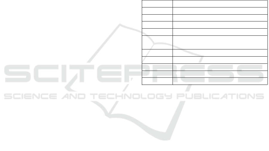
Table 2: Cross Validation for Model Selection.
Test Set Dice Coefficient Statistics
Model Size Median Min Max
U-Net 4.9M 0.628 0.594 0.685
U-Net 8.6M 0.660 0.632 0.698
U-Net 10.9M 0.665 0.600 0.701
Res. U-Net 2.7M 0.632 0.588 0.697
Res. U-Net 4.7M 0.656 0.609 0.696
Res. U-Net 7.4M 0.557 0.541 0.645
R2U-Net 3.4M 0.634 0.606 0.686
R2U-Net 6.0M 0.614 0.530 0.647
R2U-Net 9.4M 0.631 0.572 0.666
Attn. U-Net 3.1M 0.517 0.439 0.627
Attn. U-Net 4.5M 0.529 0.465 0.586
The U-Net model performed better on eosinophil
detection than the other more advanced approaches.
This could be due to the U-Net being able to accom-
modate more parameters within GPU memory limits.
The 10.9M U-Net had a slightly higher median and
maximum test dice set coefficient, but the 8.6M U-
Net had a much higher minimum value. We selected
the 8.9M U-Net since it was less complex and pro-
vided near equivalent accuracy as the 10.9M U-Net.
To establish the final 8.9M U-Net model, only train-
ing and validation sets were utilized from the 274 total
images. The size of the training set was 214 images
while the validation set size was 60 images. The re-
sulting validation Dice coefficient after training with
a similar process was 0.705. Figure 1 shows a few ex-
amples of eosinophil detections on validation set im-
ages.
3.1.3 Eosinophil Counting and Validation
Successful eosinophil segmentation is crucial to count
cells and generate per-image and per-patient features.
With the U-Net segmentation model established, we
then developed a post-processing technique to extract
the cell counts. First, the output of the U-Net model
was converted to a binary segmentation mask using
a 0.5 probability threshold. The resultant segmenta-
tion masks sometimes contained small contiguous ar-
eas or artifacts that were not eosinophils. Eosinophils
are typically 800 contiguous pixels in size, so objects
with less than 200 contiguous pixels were removed
to reduce false positive detections and still preserve
partially-detected eosinophils. The next step was per-
forming an Euclidean distance transformation in an
attempt to separate any eosinophils that may overlap
(Heinz et al., 1995). This operation reduced the size
of cells from the outside edge so that only the cen-
ters were counted. The approach is similar to erosion,
but is more computationally efficient. A distance of
eight pixels was used as the cutoff, because it reduced
the cell size by roughly 75% and can separate large
cell overlaps. Finally, the measure.label function was
applied from the Skimage package in Python. The
label() function applied a connected component la-
beling algorithm to separately label each contiguous
object in the prediction mask. The count of unique
labels is one of the outputs of this function and thus
represents the number of eosinophils detected in that
image.
Since the validation set Dice coefficient was op-
timized during model training, the entire 274 images
dataset was used to evaluate the cell counting capabil-
ity of segmentation and post-processing. The count-
ing error was estimated by subtracting actual and pre-
dicted eosinophil counts. The average eosinophil er-
ror over all 512 ×512 pixel images was −0.12 with a
standard deviation of 1.39 eosinophils. When scaled
to the size of an HPF, the average error was roughly
−2 eosinophils. As shown in Figure 2, the negative
bias was most pronounced when the true eosinophil
count was greater than 20. The requirement to diag-
nose EoE is 15 or more eosinophils within an area
roughly 16× larger, so the bias should not affect di-
agnosis. When the true eosinophil count was less than
15, minimal over-counting bias was noticed. This was
not problematic since false-positive diagnoses and
Advancing Eosinophilic Esophagitis Diagnosis and Phenotype Assessment with Deep Learning Computer Vision
47
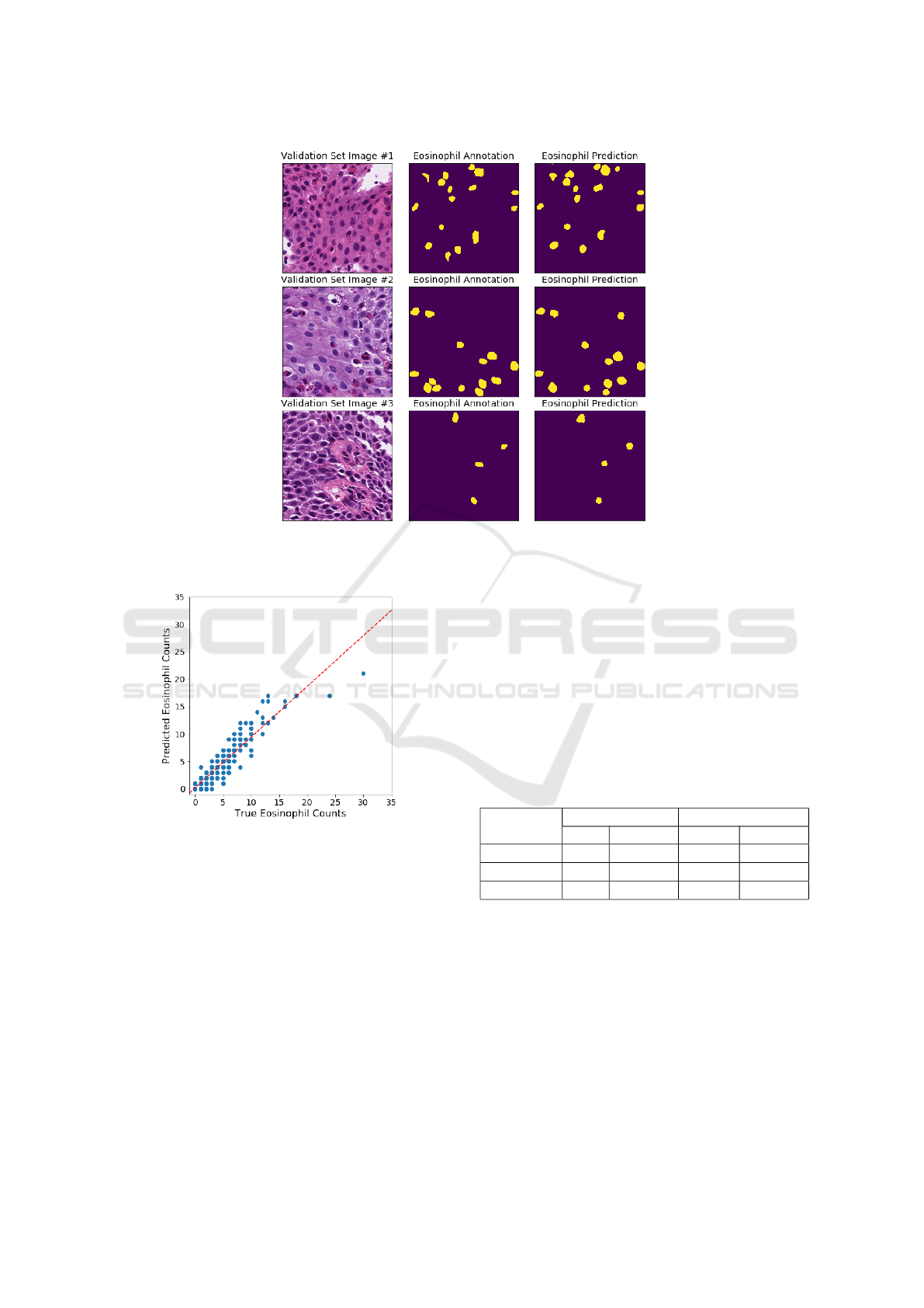
Figure 1: Examples of eosinophil detections from the U-Net model. On the left, are three input images from the validation
set. In the middle, are the ground-truth annotations. On the right, are the prediction masks.
Figure 2: Eosinophil counting errors. Each point on this
scatterplot is one of the 274 EoE patches. The dotted red
line represents the linear trend.
severity estimation are preferred over false-negatives
as it avoids under-diagnosing EoE which can lead
to worsened patient outcomes (Lipka et al., 2016).
When the number of eosinophils reach over 20 per
patch, the most likely cause of under-counting is the
inability to separate and count overlapping cells on
the prediction mask.
3.2 Classification for EoE Diagnosis
An alternative to the segmentation approach for di-
agnosis is to extract WSI patches from patients who
are EoE-diagnosed or histologically normal and train
a CNN classification model to predict EoE versus nor-
mal. Training, validation, and test sets were required
to develop this model. A total of 36 and 41 patients
were used for EoE and normal, respectively. Patches
from WSIs for patients were evenly sampled per pa-
tient and also sampled so that there was minimal class
imbalance in the training and validation sets. Table 3
shows the number of patients and patches in each data
set.
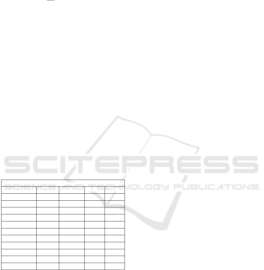
Table 3: Classification Model Data Sets.
# of Patients # of Patches
Data Set EoE Normal EoE Normal
Training 21 24 15,676 15,780
Validation 8 10 3,642 3,538
Test 7 7 7,631 3,474
A VGG16 model was trained for 12 epochs with
an Adam optimizer and learning rate of 2 ×10
−4
.
The model weights were saved that achieved the best
validation accuracy. The highest validation accuracy
achieved was 0.994. The model weights with this val-
idation accuracy achieved a test set accuracy of 0.959.
As shown in Table 4, the model rarely classified nor-
mal patches as EoE, but there were a greater number
of false-positive patches. Test set accuracies this high
are quite interesting, because it shows that EoE can be
accurately diagnosed through just a single 512 ×512
BIOIMAGING 2021 - 8th International Conference on Bioimaging
48
pixel patch. This greatly differs from the typical diag-
nosis method, so it could possibly be used to discover
new features that indicate EoE. In the Results section,
we dive deeper into the test set results and discuss the
Grad-CAM analysis.
Table 4: Test Set Confusion Matrix for Classification
Model.
Predicted
EoE Normal
True Diagnosis
EoE 7,176 455
Normal 3 3,471
4 RESULTS
In this section, we present findings generated from the
image segmentation and classification approaches.
For image segmentation, the model was applied to a
larger set of EoE patients with completed retrospec-
tive chart reviews. This led to patient-level features
for characterization of EoE that were analyzed to find
linkages with treatment and clinical phenotypes. The
image classification model produced an accurate fit
on small WSI patches. We looked further into a sin-
gle patient who had a large number of misclassified
patches and assessed Grad-CAMs to understand the
differences within their biopsy tissue sample.
4.1 Image Segmentation Results
A total of 44 EoE patients with completed retrospec-
tive chart reviews and 57 histologically normal pa-
tients were used in this section to assess diagnostic
capability and relationships with other biopsy charac-
teristics. The EoE patients were categorized into two
major phenotypes: clinical and treatment-based. The
clinical phenotypes were based on patients develop-
ing strictures vs. those with the disease remaining in-
flammatory vs. PPI-REE. Treatment phenotypes in-
cluded patients with disease that were responsive to
dairy-only (milk) elimination vs. 4 to 6 food elimina-
tion diet (4/6 FED) vs. steroids vs. unknown (where
treatment response was unclear). Biopsies from these
patients were all retrieved at the same university hos-
pital at the time of initial EoE diagnosis. To assess
the linkages between initial biopsy and phenotypes
or treatments it was important to isolate the patients
that have true initial biopsies. Table 5 shows the how
many patients were distributed in each bin for all pos-
sible categories.
Various statistics were calculated for each patient
to represent the severity and extent of EoE. Patients
had up to three WSIs each depending on how many
different esophageal locations were sampled during
the endoscopy. For all results, the HPFs from all
WSIs were aggregated for each patient and not sep-
arated by esophagus location. HPFs were not ideal
for collecting information about localized concen-
trations of eosinophils. Therefore, statistics were
also collected for 512 ×512 pixel patches to deter-
mine if there were any micro-level trends that differ
from the macro-level. Due to the small sample sizes
within the treatment and clinical phenotype categories
after splitting for initial biopsy, the non-parametric
Wilcoxon rank sum test was used to test all statisti-
cal differences between each category pair (Wilcoxon
et al., 1970). The statistics are also highly correlated
with each other within this small set of patients, so
no multivariate testing was performed. Multivariate
testing could be possible when more EoE patient re-
sponse data becomes available. The following list de-
tails some of the eosinophil statistics that were cap-
tured:
• Maximum eosinophils in HPFs
• Average eosinophil count over all HPFs
• Average eosinophil size (pixels)
• Percent of HPFs with zero eosinophils
• Percent of HPFs with ≤ 5 eosinophils
• Percent of HPFs with ≥ 15, 30, 60 eosinophils
• Maximum eosinophils in 512 ×512 patches
• Average eosinophil count over all patches
• Percent of patches with zero eosinophils
• Percent of patches with ≥ 5, 10, 15 eosinophils
4.1.1 Diagnosis, Severity, and Extent
Using the criteria of 15 or more eosinophils within an
HPF, patients were able to be diagnosed via results
obtained from the image segmentation model. Table
6 shows the classification results on the 44 and 57 pa-
tients for EoE and normal, respectively. The overall
accuracy of this approach was 99.0%. The sensitiv-
ity was 100% and the specificity was 98.2%. This
demonstrates that the automated approach was able to
adequately diagnose EoE and thus could be a useful
tool to assist pathologists.
Additionally, EoE severity can be predicted using
the eosinophil statistics. Due to the difficulty of man-
ually counting all eosinophils, pathologists typically
do not continue counting eosinophils after reaching
about 60 counted in an HPF (Collins et al., 2017).
This was not a limitation for the automated deep
learning approach. The maximum eosinophil count
can be counted as an unbounded continuous variable
Advancing Eosinophilic Esophagitis Diagnosis and Phenotype Assessment with Deep Learning Computer Vision
49
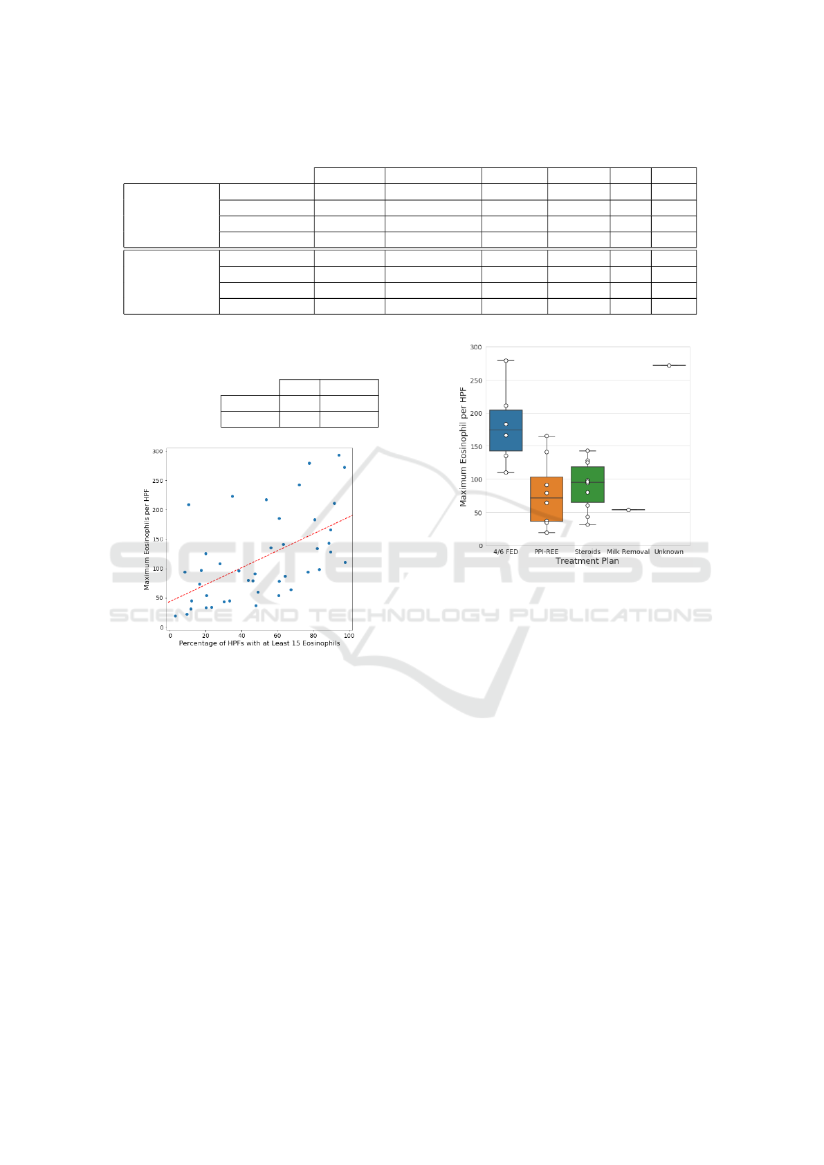
Table 5: EoE Patient Categorizations.
Treatment Plans
Phenotypes PPI-REE Milk Removal 4/6 FED Steroids Unk Total
Initial Biopsy
PPI 9 9
Inflammatory 1 4 6 11
Strictures 2 5 1 8
Total 9 1 6 11 1 28
Not Initial
PPI 0
Inflammatory 2 3 8 4 17
Strictures 1 2 3
Total 0 2 3 9 6 20
Table 6: Confusion Matrix for EoE Diagnosis.
Predicted
EoE Normal
True Diagnosis
EoE 44 0
Normal 1 56
Figure 3: EoE severity versus extent. The x-axis represents
extent, while the y-axis represent severity. The dotted red
line is the linear trend between the two factors.
which provides more fidelity over the manual method.
Similar difficulties were present when manually
estimating EoE extent. The image segmentation ap-
proach obtained counts from all HPF samples and
estimated the extent by calculating the percentage
of HPFs that exceeded a certain criteria. Figure 3
shows a scatterplot of each EoE patient’s maximum
eosinophil per HPF and percentage of HPFs with 15
or more eosinophils. Severity and extent appeared to
correlate, but there were patients who deviated from
the trend-line.
4.1.2 Linkages with Treatment Phenotypes
The goal of this subsection was to identify linkages
between collected eosinophil statistics at the time of
initial biopsy and optimal treatment plans. Treat-
ments that the patients responded to in our dataset
Figure 4: Maximum eosinophils over HPFs per patient by
treatment plan. Patients with high EoE severity tend benefit
most from 4 to 6 food elimination treatment.
were assessed at 6 or more months of follow up via
retrospective chart review. As shown in Table 5, the
sample sizes for initial biopsy patients were small but
there was enough data points within 4/6 FED, PPI-
REE, and steroids to generate statistical significance.
Figure 4 shows the maximum eosinophil count for
each patient based on their optimal treatment plan.
The maximum count was generated from all HPFs
within each patient’s WSIs. The milk removal cat-
egory did not have enough samples to evaluate and
there was also one unknown treatment. The 4/6
FED treatment appeared to correlate with higher EoE
severity. The statistical test revealed that 4/6 FED
had a significantly higher maximum eosinophil count
than PPI-REE and steroids with p-values of 0.012 and
0.006, respectively. Figure 5 shows the percentage
of HPFs that contain at least 60 eosinophils by treat-
ment plan. The 4/6 FED treatment also appeared to
correlate with higher EoE extent. There were simi-
lar trends with lower eosinophil thresholds such as 15
or 30, but 60 showed a clearer difference between the
treatments. The statistical test revealed that 4/6 FED
had a significantly higher percentage of HPFs with
BIOIMAGING 2021 - 8th International Conference on Bioimaging
50
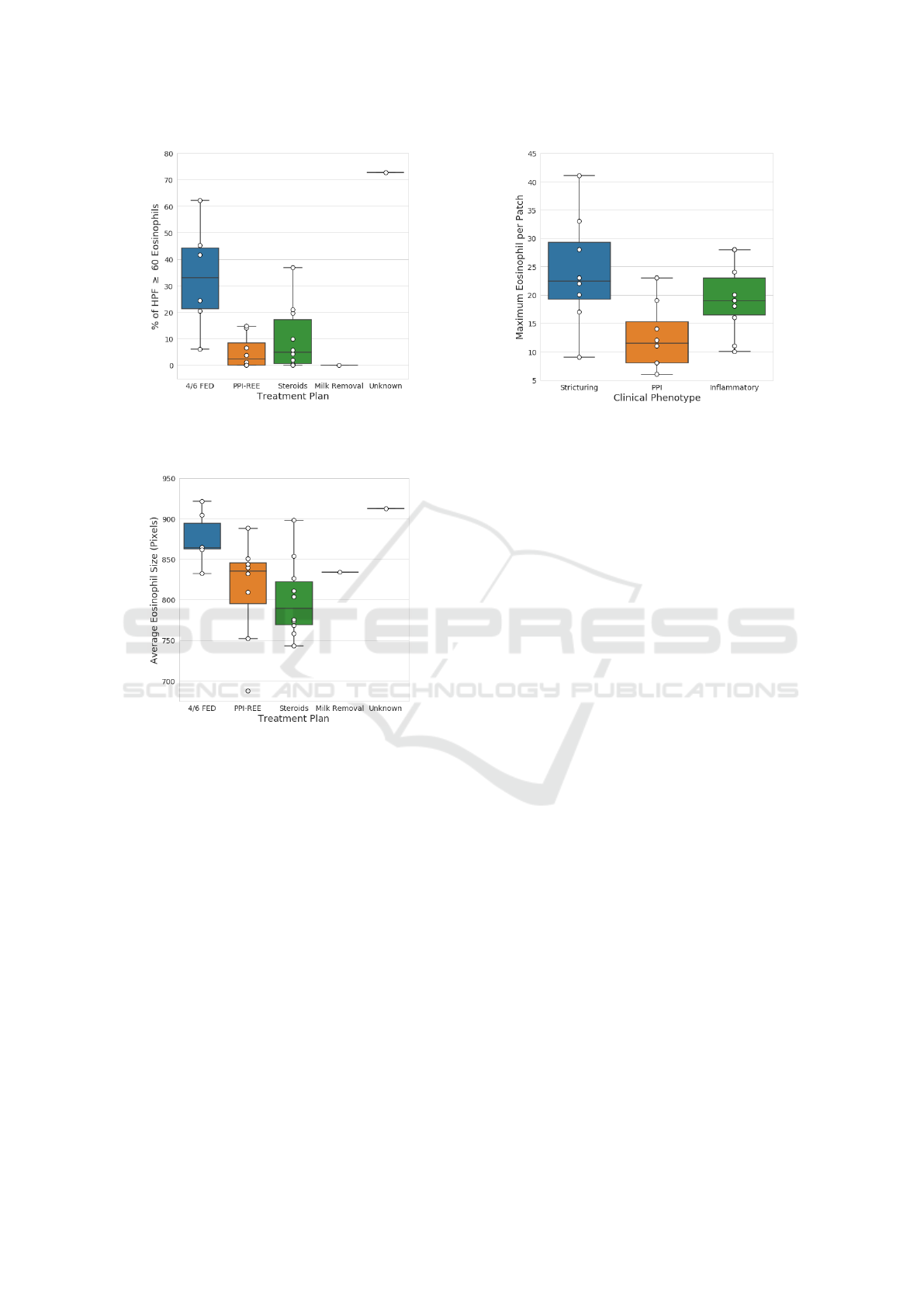
Figure 5: Percentage of HPFs with ≥ 60 eosinophils. Pa-
tients with high EoE extent tend to benefit most from 4 to 6
food elimination treatment.
Figure 6: Average eosinophil size in pixels by treatment
plan. Patients that have larger eosinophils tend to benefit
most from 4 to 6 food elimination treatment.
≥ 60 eosinophils than PPI-REE and steroids with p-
values of 0.008 and 0.015, respectively. Figure 6
shows the average eosinophil size (pixels) by treat-
ment plan. The average eosinophil size is calculated
by summing the number of eosinophil-detected pixels
in each HPF and then dividing by the predicted count.
Not only does 4/6 FED treatment seem to link with
patients with higher EoE severity and extent, but also
with the actual size of the eosinophils. The statistical
test revealed that 4/6 FED had a significantly higher
average eosinophil size than PPI-REE and steroids
with p-values of 0.033 and 0.008, respectively.
There were other variables such as the average
eosinophil count and similar statistics at the 512 ×
512 pixel patch that also showed 4/6 FED as signifi-
cantly different from PPI-REE or steroids treatment.
Figure 7: Maximum eosinophil count over patches per pa-
tient by phenotype. Patients with a low eosinophil counts in
smaller regions tend to be linked with the PPI phenotype.
4.1.3 Linkages with Clinical Phenotypes
The goal of this subsection was similar to the previ-
ous as we searched for linkages between initial biopsy
features and a patient’s clinical phenotype. While the
sample sizes were still low, the categories were fairly
well-balanced with all three ranging between 8 and
11. Figure 7 shows the maximum eosinophil count
per patient using 512 × 512 patches and by pheno-
type. The treatment phenotype findings were similar
for both HPFs and patches, but the clinical phenotype
only generated significant differences at the “micro-
level”. Therefore, the indicators of phenotypes at
the time of initial biopsy and diagnosis may only ex-
ist when examining eosinophils at a highly localized
level and not through HPFs. The statistical test re-
vealed that PPI-REE had a significantly lower max-
imum eosinophil count per patch than strictures and
inflammatory with p-values of 0.021 and 0.049, re-
spectively. Figure 7 shows the maximum eosinophil
count per patient using 512 × 512 patches by clini-
cal phenotype. This shows another example of how
patients with the PPI-REE phenotype rarely ever ex-
ceeded ten eosinophils within a 512 ×512 patch. The
median percentage for PPI was less than 1%, while
the other two had medians at roughly 4%. The sta-
tistical test revealed that PPI-REE had a significantly
lower percentage of patches with ≥ 10 eosinophils
than strictures and inflammatory with p-values of
0.034 and 0.011, respectively.
Advancing Eosinophilic Esophagitis Diagnosis and Phenotype Assessment with Deep Learning Computer Vision
51
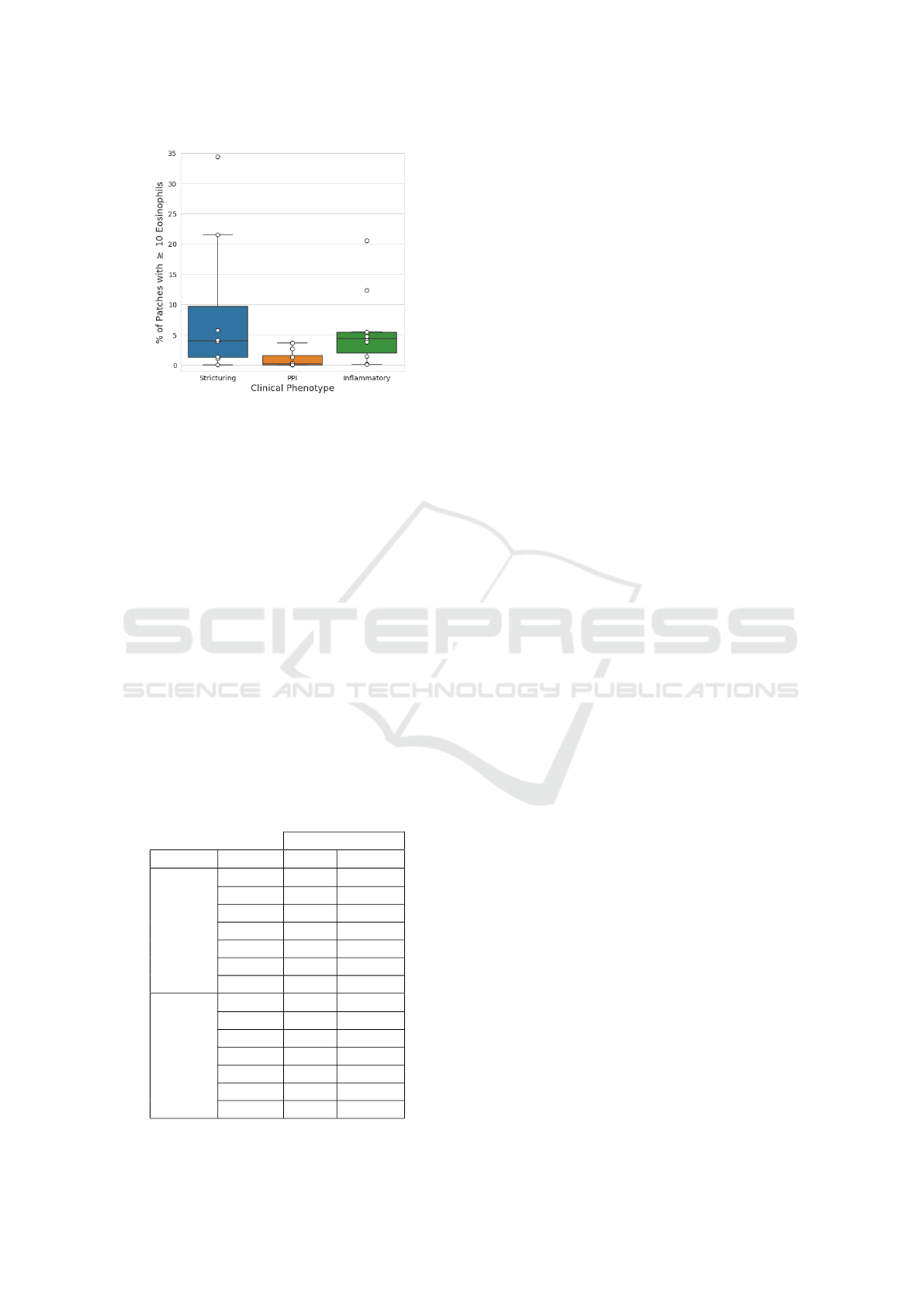
Figure 8: Percentage of patches with ≥ 10 eosinophils per
patient by phenotype. Patients with very low percentages of
patches with a large number of eosinophils tend to have the
PPI-REE phenotype.
4.2 Image Classification Results
As discussed in the Methodology section, a VGG16
CNN model was developed with training and valida-
tion data sets and then evaluated on a test set. The
training and validation sets contained EoE patients
from the 4/6 FED, PPI-REE, and steroids treatment
plans, while the test set EoE patients were from the
milk removal and unknown treatments. Overall, the
prediction accuracies were high across all three data
sets, but there was one interesting anomaly in the test
set results. Table 7 shows the classification results
from the VGG16 model by each patient from the test
set. All patients had almost all of their patches cor-
rectly classified except for EoE patient E-136. About
one-third of the WSI patches for E-136 were mis-
classified as normal, while other patients had almost
Table 7: Classification Predictions by Patient.
Prediction
Truth Patient EoE Normal
EoE
E-29 187 1
E-103 701
E-116 798
E-123 1,567 17
E-124 784 2
E-136 808 435
E-201 2,331
Normal
N16-38 450
N16-39 3 1,317
N16-40 355
N16-41 651
N16-42 285
N16-43 381
N16-44 32
100% correctly classified EoE patches. The fact that
predictions varied within one patient’s WSI was one
piece of supporting evidence that the model was not
utilizing extraneous features to classify EoE vs. nor-
mal. Examining patient E-136’s tissue sample may
be the key to determining which biopsy features were
utilized by the deep learning model. Grad-CAMs can
be utilized to visualize the important features used
in a CNN model. Grad-CAMs were produced at the
patch-level to cover E-136’s entire WSI in order to as-
sess which parts of the tissue were considered EoE or
normal. Pathologists examined the Grad-CAMs and
determined whether there was a consistent trend as-
sociated with the tissue and a prediction class. The
WSI-level Grad-CAMs were highlighting more areas
for images that had a higher number of eosinophils.
Further, the heatmaps were also focusing on areas
with cellular crowding and bottom most (basal) layer
of epithelium with images having dilated intercellular
spaces. These increased (dilated) intercellular spaces
indicate underlying cellular edema taking place due to
the inflammation caused by the disease (Collins et al.,
2017).
Figure 9 shows an example of a large tissue crop
from one on the WSIs from patient E-136. There
were large sections in the middle of the tissue sample
that the model considers normal (blue), while other
areas are predicted EoE (red). After analyzing pa-
tient E-136 and comparing to other patient’s Grad-
CAMs, it was determined the model was classify-
ing patches EoE or normal likely because of features
other than eosinophils such as cellular crowding and
basal layer of the epithelium. Another important as-
pect was that the classification model was not utiliz-
ing eosinophils to diagnose EoE. The section of tis-
sue in Figure 9 was very large (8000 × 6000 pixels)
and about half was predicted as EoE, but there were
only three eosinophils detected within this area. This
amount of eosinophils is far short of the typical diag-
nostic criteria.
5 CONCLUSION
In this paper, we present a novel approach for diag-
nosing EoE, understanding more about biopsy tissue
level features, and linking EoE biopsy features with
treatment and clinical phenotypes. This was the first
time deep learning computer vision was applied to
diagnose EoE and detect eosinophils in biopsy tis-
sue samples. The eosinophil segmentation is med-
ically critical since it can aide pathologists in di-
agnosis by automatically providing peak eosinophil
counts and knowledge of other areas requiring direct
BIOIMAGING 2021 - 8th International Conference on Bioimaging
52
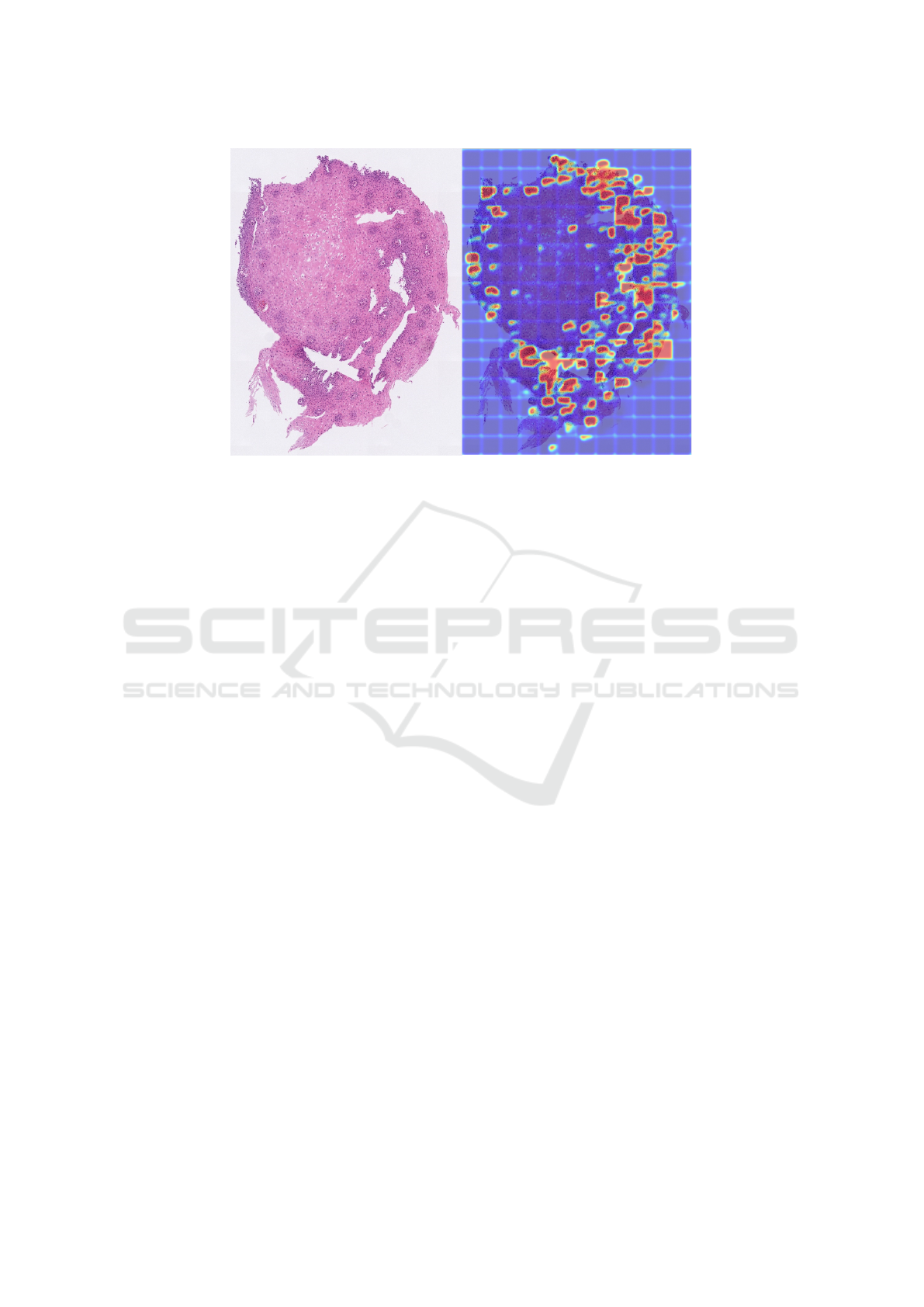
Figure 9: Grad-CAMs are applied to patches over a section of tissue from patient E-136’s WSI. On the left, is the section of
WSI tissue. On the right is the same crop of tissue, but with the Grad-CAM overlaid. This was the only EoE patient in the
test set that had large areas of tissue predicted as normal.
focus and attention. The automated assessment of
eosinophil count can also be associated with disease
severity, progression, and medically-relevant treat-
ment and clinical phenotypes. The trained U-Net im-
age segmentation model detected eosinophils within
an adequate accuracy.
Most of the patient-level eosinophil statistics can-
not be realistically captured without an automated ap-
proach. These statistics can be used to explain the
EoE severity and extent or to predict clinical and treat-
ment phenotypes. Statistical analysis revealed that
patients who eventually responded to the 4/6 FED
treatment plan had high severity and extent of EoE at
the time of initial biopsy. The PPI-REE phenotype
was found to relate with lower severity (decreased
eosinophil counts) and extent at the smaller patch
level.
In conjunction with image segmentation, image
classification was used to learn more about how
biopsy features relate to EoE. A VGG16 CNN model
was trained on a data set of EoE and normal WSI
patches and achieved highly accurate results. The
model’s performance was interesting since it was able
to predict EoE using only small patches and did not
depend solely on eosinophils for diagnosis. One EoE
patient in particular had a large section of tissue pre-
dicted as normal and this was because it had less
areas of eosinophils which lead to less activations
mapped by Grad-CAMs but also features other than
eosinophils such as cellular crowding and basal ep-
ithelial layer with some images have dilated inter-
cellular spaces were being highlighted. Basal layer
epithelium identification and its thickness along with
presence of dilated intercellular spaces representing
cellular edema are signs of inflammation caused by
EoE and have been proposed as possible diagnostic
features of the disease (Collins et al., 2017).
There are many avenues for future research in this
area. Increasing eosinophil annotations will further
improve prediction performance and enable the model
to be more robust to even slight variations in new
biopsy imagery. The sample size of patient-level data
was small due to which most of the statistical anal-
ysis was limited. There is currently a plan in place
to greatly increase the sample size of patients with
completed chart reviews. With additional data, we
will also be able to analyze eosinophil trends by the
esophageal tissue sample location. The Grad-CAM
review can be considered subjective, thus integrat-
ing Grad-CAMs with another approach that can quan-
tify cellular-level features will reduce human-injected
bias. We are in the process of developing an unsu-
pervised segmentation approach that will also be re-
viewed by pathologists to automate patch-level fea-
ture generation.
REFERENCES
Alom, M. Z., Yakopcic, C., Taha, T. M., and Asari, V. K.
(2018). Nuclei segmentation with recurrent residual
convolutional neural networks based U-Net (r2u-net).
In NAECON 2018 - IEEE National Aerospace and
Electronics Conference, pages 228–233.
Carr, S., Chan, E. S., and Watson, W. (2018). Eosinophilic
esophagitis. Allergy, Asthma & Clinical Immunology,
14(2):1–11.
Advancing Eosinophilic Esophagitis Diagnosis and Phenotype Assessment with Deep Learning Computer Vision
53

Collins, M. H., Martin, L. J., Alexander, E. S., Boyd, J. T.,
Sheridan, R., He, H., Pentiuk, S., Putnam, P. E., Abo-
nia, J. P., Mukkada, V. A., Franciosi, J. P., and Rothen-
berg, M. E. (2017). Newly developed and validated
eosinophilic esophagitis histology scoring system and
evidence that it outperforms peak eosinophil count for
disease diagnosis and monitoring. Diseases of the
Esophagus : Official Journal of the International So-
ciety for Diseases of the Esophagus, 30(3):1–8.
Dellon, E. S. (2014). Epidemiology of eosinophilic
esophagitis. Gastroenterology Clinics, 43(2):201–
218.
Dellon, E. S., Kim, H. P., Sperry, S. L., Rybnicek, D. A.,
Woosley, J. T., and Shaheen, N. J. (2014). A pheno-
typic analysis shows that eosinophilic esophagitis is
a progressive fibrostenotic disease. Gastrointestinal
Endoscopy, 79(4):577–585.
Eelbode, T., Bertels, J., Berman, M., Vandermeulen, D.,
Maes, F., Bisschops, R., and Blaschko, M. B. (2020).
Optimization for medical image segmentation: The-
ory and practice when evaluating with dice score or
jaccard index. IEEE Transactions on Medical Imag-
ing.
Furuta, G. T., Liacouras, C. A., Collins, M. H., Gupta,
S. K., Justinich, C., Putnam, P. E., Bonis, P., Hassall,
E., Straumann, A., Rothenberg, M. E., et al. (2007).
Eosinophilic esophagitis in children and adults: A sys-
tematic review and consensus recommendations for
diagnosis and treatment: Sponsored by the Ameri-
can Gastroenterological Association (AGA) institute
and north American society of pediatric gastroenterol-
ogy, hepatology, and nutrition. Gastroenterology,
133(4):1342–1363.
Godwin, B., Wilkins, B., and Muir, A. B. (2020). Eoe dis-
ease monitoring: Where we are and where we are
going. Annals of Allergy, Asthma & Immunology,
124(3):240–247.
Habibzadeh, M., Jannesari, M., Rezaei, Z., Baharvand, H.,
and Totonchi, M. (2018). Automatic white blood cell
classification using pre-trained deep learning models:
Resnet and inception. In Tenth International Confer-
ence on Machine Vision (ICMV 2017), volume 10696,
page 1069612. International Society for Optics and
Photonics.
Heinz, B., Gil, J., Kirkpatrick, D., and Werman, M. (1995).
Linear time Euclidean distance transform algorithms.
IEEE Transactions on Pattern Analysis and Machine
Intelligence, 17(5):529–533.
Kingma, D. and Ba, J. (2014). Adam: A method for
stochastic optimization. International Conference on
Learning Representations.
Kumar, N., Verma, R., Anand, D., Zhou, Y., Onder, O. F.,
Tsougenis, E., Chen, H., Heng, P. A., Li, J., Hu, Z.,
et al. (2019). A multi-organ nucleus segmentation
challenge. IEEE Transactions on Medical Imaging.
Liacouras, C. A., Furuta, G. T., Hirano, I., Atkins, D.,
Attwood, S. E., Bonis, P. A., Burks, A. W., Chehade,
M., Collins, M. H., Dellon, E. S., et al. (2011).
Eosinophilic esophagitis: Updated consensus recom-
mendations for children and adults. Journal of Allergy
and Clinical Immunology, 128(1):3–20.
Liang, G., Hong, H., Xie, W., and Zheng, L. (2018). Com-
bining convolutional neural network with recursive
neural network for blood cell image classification.
IEEE Access, 6:36188–36197.
Lipka, S., Kumar, A., and Richter, J. E. (2016). Impact of
diagnostic delay and other risk factors on eosinophilic
esophagitis phenotype and esophageal diameter. Jour-
nal of Clinical Gastroenterology, 50(2):134–140.
Milletari, F., Navab, N., and Ahmadi, S.-A. (2016). V-
net: Fully convolutional neural networks for volumet-
ric medical image segmentation. In 2016 Fourth Inter-
national Conference on 3D Vision (3DV), pages 565–
571. IEEE.
Nielsen, J. A., Lager, D. J., Lewin, M., Rendon, G., and
Roberts, C. A. (2014). The optimal number of biopsy
fragments to establish a morphologic diagnosis of
eosinophilic esophagitis. The American Journal of
Gastroenterology, 109(4):515.
Oktay, O., Schlemper, J., Folgoc, L. L., Lee, M., Heinrich,
M., Misawa, K., Mori, K., McDonagh, S., Hammerla,
N. Y., Kainz, B., et al. (2018). Attention u-net: Learn-
ing where to look for the pancreas. International Con-
ference on Medical Imaging with Deep Learning.
¨
Ozyurt, F. (2019). A fused CNN model for WBC detection
with MRMR feature selection and extreme learning
machine. Soft Computing, pages 1–10.
Reed, C. C., Koutlas, N. T., Robey, B. S., Hansen, J.,
and Dellon, E. S. (2018). Prolonged time to diag-
nosis of eosinophilic esophagitis despite increasing
knowledge of the disease. Clinical Gastroenterology
and Hepatology: the Official Clinical Practice Jour-
nal of the American Gastroenterological Association,
16(10):1667.
Ronneberger, O., Fischer, P., and Brox, T. (2015). U-
Net: Convolutional networks for biomedical image
segmentation. In International Conference on Medi-
cal image computing and computer-assisted interven-
tion, pages 234–241. Springer.
Rosenberg, H. F., Dyer, K. D., and Foster, P. S. (2012).
Eosinophils: changing perspectives in health and dis-
ease. Nature Reviews Immunology, 13(1):9–22.
Runge, T. M., Eluri, S., Cotton, C. C., Burk, C. M.,
Woosley, J. T., Shaheen, N. J., and Dellon, E. S.
(2017). Causes and outcomes of esophageal perfo-
ration in eosinophilic esophagitis. Journal of Clinical
Gastroenterology, 51(9):805.
Russakovsky, O., Deng, J., Su, H., Krause, J., Satheesh, S.,
Ma, S., Huang, Z., Karpathy, A., Khosla, A., Bern-
stein, M., et al. (2015). Imagenet large scale visual
recognition challenge. International journal of com-
puter vision, 115(3):211–252.
Selvaraju, R. R., Cogswell, M., Das, A., Vedantam, R.,
Parikh, D., and Batra, D. (2017). Grad-CAM: Visual
explanations from deep networks via gradient-based
localization. In Proceedings of the IEEE International
Conference on Computer Vision, pages 618–626.
Simonyan, K. and Zisserman, A. (2015). Very deep con-
volutional networks for large-scale image recognition.
In International Conference on Learning Representa-
tions.
BIOIMAGING 2021 - 8th International Conference on Bioimaging
54

Sudre, C. H., Li, W., Vercauteren, T., Ourselin, S., and Car-
doso, M. J. (2017). Generalised dice overlap as a deep
learning loss function for highly unbalanced segmen-
tations. In Deep learning in medical image analysis
and multimodal learning for clinical decision support,
pages 240–248. Springer.
Tran, T., Kwon, O.-H., Kwon, K.-R., Lee, S.-H., and Kang,
K.-W. (2018). Blood cell images segmentation using
deep learning semantic segmentation. In 2018 IEEE
International Conference on Electronics and Commu-
nication Engineering (ICECE), pages 13–16. IEEE.
Wilcoxon, F., Katti, S., and Wilcox, R. A. (1970). Critical
values and probability levels for the Wilcoxon rank
sum test and the Wilcoxon signed rank test. Selected
tables in mathematical statistics, 1:171–259.
Wilson, J. M. and McGowan, E. C. (2018). Diagnosis and
management of eosinophilic esophagitis. Immunology
and allergy clinics of North America, 38(1):125.
Zhang, Z., Liu, Q., and Wang, Y. (2018). Road extraction
by deep residual U-Net. IEEE Geoscience and Remote
Sensing Letters, 15(5):749–753.
Advancing Eosinophilic Esophagitis Diagnosis and Phenotype Assessment with Deep Learning Computer Vision
55
