
Prediction of Cotton Field on Integrated Environmental Data
Sarthak Mishra
1
, Long Ma
2
and Nischal Aryal
2
1
Department of Computer Science, University of Illinois at Urbana Champaign, Urbana, IL, U.S.A.
2
Department of Computer Science, Troy University, Troy, AL, U.S.A.
Keywords: Agriculture, Crop Production, Cotton Yield, Prediction, Regression.
Abstract: The agriculture and farming industry plays a vital role in the economy. However, the importance of agriculture
cannot be fully quantified in terms of its economic profit. Agriculture affecting global hunger is a much more
sensitive and vital topic. One of the leading reasons for this is un-improvised crop production. Crop production
is affected by various factors, and monitoring those factors is the key to solving the problem. This paper
describes a comprehensive experiment predicting the cotton yield under various environments, such as Acres
Harvested, Acres Planted, Soil pH, Bulk Density, Clay-High, Clay-Low, Organic-Carbon, and Water-Area.
1 INTRODUCTION
Agriculture production is known to be affected by
various factors, such as temperature. With a slight
change of these factors, there can be considerable
variations on the crop’s net yield. Most of these
factors are environmental; for instance, rainfall and
temperature change seasonally, whereas factors like
Bulk Density and water-area of the soil change
slowly. To accurately quantify the effects of the
environmental factors on crop yield, type of crop and
the irrigation practices of the chosen crop must
remain constant.
The problem then reduces to predicting the amount
of crop yield based on the environmental factors.
Statistically, this problem boils down to a regression
task. Hence, our research focuses on discovering any
quantifiable co-relations between these
environmental factors and the yield of the crop.
Intuitively there seems to be a cause-and-effect
relation between these environmental factors and the
crop yield. This paper aims to verify a presence
statistical relationship between these factors and the
crop yield.
One of state-of-art machine learning classifiers has
been applied to the research to improve the
performance of the model, we will have to choose the
dependent entities carefully. The dependent entities
chosen for our study are Acres Harvested, Acres
Planted, Soil pH, Bulk Density, Clay-High, Clay-
Low, Organic-Carbon, and Water-Area.
The rest of the paper is organized as follows. Next
section discusses the data collection. In the third
section, we describe the data preparation and
proposed method. The fourth section illustrates
several comprehensive experiments for crop yield
prediction. At last, our work is concluded, and future
work is presented.
2 DATA PREPARATION
The data is collected from several web databases
(ISRIC WOSIS). The primary source we used in our
research is the USDA (United States Department of
Agriculture) database. The weather data is derived
from the weather API. The goal of this project is to
predict the cotton yield using soil type and weather
data. By profiling the column and the row of the
extracted data, two master tables and five child tables
were created.
2.1 Parent Table
The sources of data of these tables are the USDA
database and ISRIC WOSIS database. After
exhaustively collecting the data from the
websites www.ers.usda.gov/data-products and
https://websoilsurvey.sc.egov.usda.gov/App/WebSoi
lSurvey.aspx.
We divided the records into two main tables. These
tables stored the exact copy of online data. The two
master tables planned are soil table and crop table.
Mishra, S., Ma, L. and Aryal, N.
Prediction of Cotton Field on Integrated Environmental Data.
DOI: 10.5220/0010240707810786
In Proceedings of the 13th International Conference on Agents and Artificial Intelligence (ICAART 2021) - Volume 2, pages 781-786
ISBN: 978-989-758-484-8
Copyright
c
2021 by SCITEPRESS – Science and Technology Publications, Lda. All rights reserved
781

▪ Soil table: stores the bulk of information
extracted from the given data sources.
▪ Crop table: the cotton plant is one of the most
complex structured plants. The life cycle of
cotton is found to be significantly changing
based on environmental conditions. Thus,
making this plant uniquely suitable for our
project. The root length of the cotton plant
varies from 30inch to 38 inches. Hence for the
analysis of this paper, the standard length of
80cm (31.50 inches) is taken. The information
stored in this table is the yield of cotton in
various counties of the united states of
America. This data is extracted from the USDA
database. This table also stores the Acres
Harvested and Acres Planted of cotton.
2.2 Child Table
The grain of data for these tables are derived from the
master tables. For the informational extraction and
consistency in the data lineage, a child table only has
one Master table as the source. There were 6 child
tables to store seven of our labels used for regression
analysis. All the below mentioned table are derived
from Soil Table:
▪ Soil Classification table: stores the place’s
location, namely Latitude and longitude
with the soil type. The metadata for this table
is Latitude, Longitude, and Soil Type.
▪ Site Characteristic table: stores the location,
namely Latitude and longitude with Soil
organic carbon stock in tonnes per hectare.
The metadata for this table is Latitude,
Longitude, Depth to bedrock.
▪ Soil Water: the metadata of the Soil Water
table is Latitude, Longitude, and Volumetric
water content at wilting point pF 4.2(WWP).
▪ Climate Data: the metadata of the Climate
Data is Latitude, Longitude, High
Temperature in Degrees, Low Temperature
in Degrees, and Average rainfall in inch.
▪ Physical Soil Properties table: the physical
soil properties of a location are divided into
four different types. These tables store the
location of the place namely Latitude and
longitude with different Physical attributes.
o Bulk density: The metadata of
the bulk density table is
Latitude, Longitude, and bulk
density.
o Coarse fragments: the metadata
of the Coarse fragments table is
Latitude, Longitude, and the
volumetric percent of the
fragments in 80cm depth.
o Bulk density: the metadata of
the bulk density table is
Latitude, Longitude, and bulk
density.
o Soil texture fraction silt in
percentage: the metadata of the
Soil texture slit table is
Latitude, Longitude, and the slit
in percentage at 80cm depth.
o Soil texture fraction sand in
percentage: the metadata of the
Soil texture sand table is
Latitude, Longitude, and the
sand in percentage at 80 cm
depth.
▪ Chemical Soil Properties: the chemical
Soil properties tables store the
information about the place like
Latitude, Longitude, and several
chemical properties.
o Cation exchange capacity: the
Cation exchange capacity
table's metadata is Latitude,
Longitude, and fine earth
fraction in cmolc/kg at 80cm
o Total nitrogen: the metadata of
the Total nitrogen table is
Latitude, Longitude, and the
fine earth fraction (80cm).
o Soil organic carbon content:
the metadata of the soil organic
carbon content table is Latitude,
Longitude, and fine earth
fraction in permilles at 80cm.
o Soil pH in H2O: the metadata
of the Soil pH in the H2O table
is Latitude, Longitude, and pH
in H2O at 80cm.
o Soil pH in Kcl: the metadata of
the Soil pH in the Kcl table is
Latitude, Longitude, and pH in
Kcl at 80cm.
2.2.1 Association Table
Association Table is the penultimate table for this
project. The models were created as part of this
project feed of the association table. There was a
significant challenge to meet the purpose of this table.
The challenge was to bind the data between the child
table and the crop master table. The content of child
tables was uniquely identified using the latitude and
ICAART 2021 - 13th International Conference on Agents and Artificial Intelligence
782

longitude of a place, whereas the crop table was being
uniquely identified using the county's name. This
structure created a lack of shared key columns
between these tables. To mitigate this problem, we
took the average of all the child table's data in the
rough square boundary of a county and took this as
the final data.
The lack of information derived from the weather
table is not being included in our association table.
The latitude and longitude of the weather table were
missing for many counties. The metadata of this table
is County Name, State, Acres Harvested, Acres
Planted, Yield, Soil pH, Bulk Density, Clay-High,
Clay-Low, Organic-Carbon, and Water-Area.
2.2.2 Data Definition
▪ Soil-pH: indicates the acidity or alkalinity of
the soil. The PH unit is called the pH unit, and
it represents the negative logarithm of the
hydrogen ion concentration. The pH ranges
from 0 to 14. The pH of the soil is known to
affect the yield to a great degree. The
measurement of soil acidity or alkalinity is like
a doctor's measurement of a patient's
temperature. Changes in the acidity of soils
may change the availability to plants of
different nutrients in different ways
(Allaway,1957).
▪ Bulk Density: the calculation of the
compactness of the soil. It is the dry weight of
soil divided by its volume. The unit of Bulk
Density is g/cm3. The bulk density of the soil
affects the growth of the roots thereby affecting
the overall yield of the crop. Roots growing in
compacted soils can traverse otherwise
impenetrable soil using bio pores and cracks
and thus gain access to a more extensive
reservoir of water and nutrients (Stirzaker,
Passioura, and Wilms, 1996).
▪ Organic-Carbon: a measurable component of
soil organic matter. Organic Carbon is the
primary source of energy for soil
microorganisms.
▪ Water-Area: the number of miles of water body
contained in that area. The unit of measurement
is in miles.
▪ Crop yield: the quantification of the amount of
produce harvested per unit land.
▪ Acres Planted: the acres of land used for cotton
plantation.
▪ Acres Harvested: the acres of land where cotton
was harvested.
▪ Clay-High: represents the percentage of clay
with high plasticity. A clay–water system of
high plasticity requires more force to deform it
and deforms to a greater extent without
cracking than one of low plasticity, which
deforms more easily and ruptures sooner
(Brownell, 1977)
▪ Clay-Low: represents the percentage of clay
with high plasticity. The hydraulic conductivity
of the soil is known to be affected by the
plasticity of clay (Allen, 2005)
3 PROPOSED METHOD
3.1 Data Profiling and Modelling
After brief profiling, a supervised learning model will
be appropriately applied. There are two types of
learning approaches in supervised learning.
▪ Regression Analysis
▪ Classification Problem
The problem of our interest falls under the realm of
regression learning.
3.2 Regression Analysis
The central concept of this method is to find an
algebraic relationship between the dependent and the
independent variables. A model of the relationship is
hypothesized and estimates of the parameter values
are used to develop an estimated regression equation
(
Ostertagováa, 2012). This experiment will be using
Linear Regression.
Linear regression is a statistical tool for forming
the relationship between some "explanatory"
variables and some real-valued outcome (Shalev-
Shwartz and Ben-David, 2014). This research uses
nonlinear polynomial predictors. A nonlinear
polynomial predictor is a one-dimensional
polynomial function of degree n, that is
p(x) = a
0
+ a
1
x + a
2
x
2
+ ꞏ ꞏ ꞏ + a
n
x
n
(1)
where (a
0
, a
1
, a
2
, ꞏ ꞏ ꞏ, a
n
) is a vector of coefficients of
size n + 1(Shalev-Shwartz and Ben-David, 2014).
To implement this method, we have used [Acres
Harvested, Acres Planted, Soil pH, Bulk Density,
Clay-High, Clay-Low, Organic-Carbon, and Water-
Area] as our independent variable and [crop yield] as
our dependent variable. The dichotomy of data was
created to separate the test and train data. Out of all
50 states, 'Alabama's data was used to test the
Prediction of Cotton Field on Integrated Environmental Data
783
hypothesis. The experiment uses a training set that is
better fitted using a 5th-degree polynomial predictor
than using a linear predictor.
y=a
0
+a
1
x
1
+a
2
x
2
+...+a
n-2
x
6
5
+a
n-1
x
7
5
+a
n
x
8
5
(2)
For this experiment: y is the Yield of cotton; a
0
is
the intercept; a
1
, a
2
, a
3
... a
n,
is the coefficient for Acres
Harvested, Acres Planted, Soil pH, Bulk Density,
Clay-High, Clay-Low, Organic-Carbon, and Water-
Area in 5th degree polynomial predictor. These are
called model coefficients. These values are generated
during model fitting and can be used for making
predictions.
This experiment used the linear regression
function that was packaged in the scikit-learn to
create the model. The scatter plots were generated
using Matplotlib.
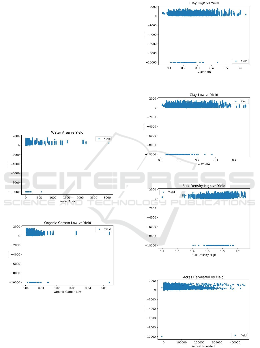
Figure 1: Scatterplot Water area vs Yield.
Figure 2: Organic Carbon vs Yield.
Figure 3: Scatterplot Clay High vs Yield.
Figure 4: Scatterplot Clay Low vs Yield.
Figure 5: Scatterplot Bulk Density vs Yield.
Figure 6: Scatterplot Acres Harvested vs Yield.
ICAART 2021 - 13th International Conference on Agents and Artificial Intelligence
784
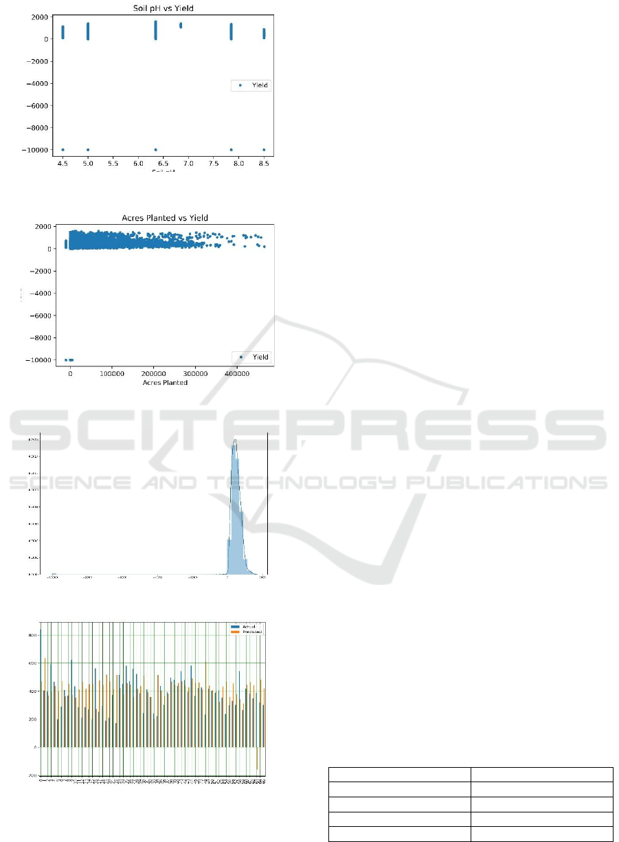
Figure 7: Scatterplot Soil pH vs Yield.
Figure 8: Scatterplot Acres Planted vs Yield.
Figure 9: Distribution of Yield.
Figure 10: Actual Data VS Predicted Data.
The first figure has the data that is cultured
between 0-250 units. In Figure 2, our data is
concentrated between 0-0.01 units for organic carbon.
We can infer that cotton's yield is maximized when
organ carbon is less than 0.01 units. Figure 3 and
figure 4 display that data on clay high and clay low is
spread around 0.1-0.6 units and 0.0-0.4 units,
respectively. Next, figure 5 shows that our data is
concentrated around 1.5 to 1.65 units. We can infer
that the precision of prediction will be in this region.
Also, figure 6 presents cotton harvested in less than
100000 acres; our data yield is more concentrated. In
the following figure, we find bands of 6 ph. values
that are affecting the yield. Figure 8 includes cotton
planted in less than 100000 acres; our data yield is
more concentrated. Figure 9 illustrates that our data
of cotton yield is distributed around 800 units.
Figure 10 compares the actual data and the
predicted data. The mean accuracy of this comparison
was 82%. It also tells the actual value of the
dependent variable [Yield] and the dependent
variable [Yield] predicted by the model created in this
experiment.
3.3 Results Analysis
For the experiment, we are using the coefficient of
Determination as the evaluation metric. The
coefficient of determination, a.k.a. R2, is well-
defined in linear regression models and measures the
proportion of variation in the dependent variable
explained by the predictors included in the model
(Zhang, 2017). The value of R2 ranges from 0 to 1- 0
being the worst and 1 being the best value.
R-squared measures of 0.86 represent the model
used for this experiment was of high accuracy. Hence,
using the knowledge from the above several
experiments we find that there is a quantifiable
correlation between environmental factors and the
yield of cotton. This experiment also finds that it is
feasible to predict the return of cotton-based on
several environmental factors. Hence, we conclude
that there is enough evidence to support our initial
hypothesis that there is a quantifiable relationship
between environmental parameters like pH, bulk
density, acres harvest, and planted with the Yield.
Table 1: Results of the Experiment.
Absolute Mean 128.51
Root Mean square
d
171.18
Absolute Median 87.65
Variance score 0.78
R2 score 0.86
Prediction of Cotton Field on Integrated Environmental Data
785

4 CONCLUSIONS
From the experiments above we conclude that it is
convincing to predict the yield of crops with good
accuracy based on environmental factors. Introducing
new factors will expand the model as well as improve
the accuracy of the model.
In the future, we are planning to collect more data
for several countries and improvise the model. We
plan to include weather data in the model as we
suspect this will improve the accuracy of the model.
REFERENCES
Allaway, W. H. 1957. pH, soil acidity and plant growth.
Pp. 67–79 in Soils: the 1957 yearbook of agriculture.
United States Department of Agriculture
Allen, Whitney M., 2005. The relationship between
plasticity ratio and hydraulic conductivity for bentonite
clay during exposure to synthetic landfill
leachate. Graduate Theses and Dissertations.
https://scholarcommons.usf.edu/etd/2772
Brownell W.E., 1977. Structural clay products Applied
Mineralogy, Springer, Berlin, vol. 9.
Zhang (2017) A Coefficient of Determination for
Generalized Linear Models, The American Statistician,
71:4, 310-316, DOI: 10.1080/00031305.2016.1256839
ISRIC WOSIS.https://data.isric.org/geonetwork/srv/eng/
catalog.search#/home.
Laliberte, G.E. and Corey, A.T. (1966) Hydraulic
properties of disturbed and undisturbed clays, ASTM,
STP. 417.
Ostertagováa, E. (2012). Modelling using polynomial
regression.
Shalev-Shwartz, S., & Ben-David, S. (2014).
Understanding Machine Learning - From Theory to
Algorithms, Cambridge University Press. Cambridge
Stirzaker, R. J., Passioura, J. B. & Wilms, Y. 1996., Soil
structure and plant growth: Impact of bulk density
and biopores. PlantSoil 185, 151–162.
https://doi.org/10.1007/BF02257571
USDA. data-products. United States Department of
Agriculture. www.ers.usda.gov/data-products.
Websoilsurvey.https://websoilsurvey.sc.egov.usda.gov/Ap
p/WebSoilSurvey.aspx.
Weather API. https://openweathermap.org/api.
ICAART 2021 - 13th International Conference on Agents and Artificial Intelligence
786
