YOdar: Uncertainty-based Sensor Fusion for Vehicle Detection

with Camera and Radar Sensors

Kamil Kowol

, Matthias Rottmann

, Stefan Bracke

and Hanno Gottschalk

School of Mathematics and Natural Sciences, University of Wuppertal, Gaußstraße 20, Wuppertal, Germany

Chair of Reliability Engineering and Risk Analytics, University of Wuppertal, Gaußstraße 20, Wuppertal, Germany

Keywords:

Uncertainty in AI, Machine Learning, Sensor Fusion, Vehicle Detection at Night.

Abstract:

In this work, we present an uncertainty-based method for sensor fusion with camera and radar data. The

outputs of two neural networks, one processing camera and the other one radar data, are combined in an

uncertainty aware manner. To this end, we gather the outputs and corresponding meta information for both

networks. For each predicted object, the gathered information is post-processed by a gradient boosting method

to produce a joint prediction of both networks. In our experiments we combine the YOLOv3 object detection

network with a customized 1D radar segmentation network and evaluate our method on the nuScenes dataset.

In particular we focus on night scenes, where the capability of object detection networks based on camera

data is potentially handicapped. Our experiments show, that this approach of uncertainty aware fusion, which

is also of very modular nature, signiﬁcantly gains performance compared to single sensor baselines and is in

range of speciﬁcally tailored deep learning based fusion approaches.

1 INTRODUCTION

One of the biggest challenges for computer vision

systems in automated driving is to recognize the cars

environment appropriately in any given situation. The

data of different sensors has to be interpreted correctly

while operating with limited amount of computing re-

sources. Besides dense trafﬁc, different weather con-

ditions like sun, heavy rain, fog and snow are chal-

lenging for state-of-the-art computer vision systems.

Previous studies show that the use of more than one

sensor, the so called sensor fusion, leads to an im-

provement in object detection accuracy, e.g. when

combining camera and lidar sensors (Silva et al.,

2018; Wu et al., 2017; Liu et al., 2017; Hansen and

Underwood, 2017; Gu et al., 2019). Up to now,

datasets containing real street scenes using radar data

and another sensor are rather the exception, although

synthetic data with different sensors, such as cam-

era and radar sensors, can be generated using simu-

lators like CARLA (Dosovitskiy et al., 2017) or LS-

GVL (Rong et al., 2020).

With the publication of the nuScenes dataset (Cae-

sar et al., 2020), the scientiﬁc community obtained ac-

cess to real street scenes recorded with different sen-

sors including radar. In total there are 5 radar sen-

sors distributed around the car that generate the data.

Ever since, the number of published papers dealing

with sensor fusion combining radar with other sen-

sors with the help of the nuScenes dataset has in-

creased, see e.g. (John and Mita, 2019; Nobis et al.,

2019; P

erez et al., 2019). We now brieﬂy review these

approaches. The authors of (John and Mita, 2019)

propose an object detection convolutional neural net-

work (CNN) named RVNet which is equipped with

two input branches and two output branches. One in-

put branch processes image data, the other one radar

data. Similarly to YOLOv3 (Redmon and Farhadi,

2018), the network utilizes two output branches to

provide bounding box predictions, i.e., one branch is

supposed to detect smaller obstacles, the other one

larger obstacles. The authors conclude that radar fea-

tures are useful for detecting on-road obstacles in a

binary classiﬁcation framework. On the other hand

the features extracted from radar data seem not to be

useful in a multiclass classiﬁcation framework due to

the sparsity of the data.

Another deep-learning-based radar and camera

sensor fusion for object detection is the CRF-Net

(CameraRadarFusionNet) (Nobis et al., 2019) , which

automatically learns at which level the fusion of both

sensor data is most beneﬁcial for object detection.

The CRF-Net uses a so-called BlackIn training strat-

egy and combines a RetinaNet (VGG backbone), a

Kowol, K., Rottmann, M., Bracke, S. and Gottschalk, H.

YOdar: Uncertainty-based Sensor Fusion for Vehicle Detection with Camera and Radar Sensors.

DOI: 10.5220/0010239301770186

In Proceedings of the 13th International Conference on Agents and Artiﬁcial Intelligence (ICAART 2021) - Volume 2, pages 177-186

ISBN: 978-989-758-484-8

177

custom-designed radar network and a Feature Pyra-

mid Network (FPN) for classiﬁcation and regres-

sion problems. The main branch is composed of

ﬁve VGG-Blocks, every block receives pre-processed

radar and image data for further processing which is

forwarded to the FPN-Blocks. The network is tested

on the nuScenes dataset and a self-build one. The au-

thors provide evidence that the BackIn training strat-

egy leverages the detection score of a state-of-the-art

object detection network.

Furthermore, a fusion approach for lidar and radar

is introduced in (P

erez et al., 2019). This approach

is designed for multi-class object detection of pedes-

trian, cyclist, car and noise (empty region of interest)

classes. To this end, lidar and radar data are ﬁrst pro-

cessed individually. The lidar branch detects objects

and tracks them over time. On the other hand, the

radar branch provides the object classiﬁcation, where

three independent fast Fourier transforms (FFTs) are

applied on the range-Doppler-angle spectrum. After

time synchronisation the two branches are merged, re-

sulting in regions of interest. These regions are fed to

the CNN, based on the VGGNet architecture, which

computes the classes probabilities. Since this ap-

proach works well for vehicle and noise classiﬁcation

but has problems with pedestrians and cyclist classes

the network was improved by applying a tracking ﬁl-

ter on top of the classiﬁer. They used a Bayes ﬁlter

which improved the classiﬁcation performance for the

two challenging classes.

In summary, the works presented (John and Mita,

2019; Nobis et al., 2019) aim at simultaneously fusing

and interpreting image and radar data within a CNN.

In (P

erez et al., 2019), lidar and radar data are ﬁrst

fused and afterwards a CNN processes the fused in-

put. While these approaches are beneﬁcial with re-

spect to maximizing performance, they require addi-

tional fallback solutions in case that a sensor drops

out. Also in contrast to other sensor fusion solutions,

our approach preserves the option to use both net-

works redundantly. In this way, indications of only

one of the networks can be used for scenario construc-

tions that are alternative to the main scenario provided

by the fusion approach.

It also seems inevitable that sensor fusion ap-

proaches require additional uncertainty measures to

verify the quality of the developed methods and net-

works. A tool for semantic segmentation called

MetaSeg that estimates prediction quality on segment

level was introduced in (Rottmann et al., 2020) and

extended in (Maag et al., 2020; Rottmann and Schu-

bert, 2019; Schubert et al., 2020). It learns to pre-

dict whether predicted components intersects with the

ground truth or not, which can be viewed as meta clas-

sifying between two classes (IoU = 0 and IoU > 0).

To this end, metrics are derived from the CNN’s

output and pass them on to another meta-classiﬁer.

This work of false positive detection was extended

in (Chan et al., 2020) where the number of over-

looked objects was reduced by only paying with a

few additional false positives. The overproduction of

false positives is suppressed by MetaSeg. Following

these approaches for uncertainty quantiﬁcation, we

use metrics from the output of two CNNs. We pass

them through to a gradient boosting classiﬁer, which

reduces the number of false positive predictions. In

addition, by reducing the score threshold for object

detection, we are able to improve over the perfor-

mance of the respective single sensor networks.

In our tests, we utilize a YOLOv3 (Redmon and

Farhadi, 2018) as a state-of-the-art object detection

network to process the camera data and complement

this with a custom-designed CNN that performs a

1D binary segmentation which is supposed to detect

obstacles. Further downstream of our computer vi-

sion pipeline we introduce a very general uncertainty-

based fusion algorithm. Based on the predictions of

both CNNs and their uncertainties as well as other

geometrical meta-information, the fusion algorithm

learns to provide a prediction by means of a struc-

tured dataset. In our experiments we demonstrate for

the case of street scenes recorded at night, that this ap-

proach signiﬁcantly improves the object detection ac-

curacy. Furthermore, both networks only show mod-

erate correlation which further supports our safety ar-

gument.

Outline. The remainder of this work is organized

as follows. In Section 2 we brieﬂy describe the char-

acteristics of different sensors used for perception in

automated driving. In Section 3 we introduce our 1D

segmentation network for the detection of vehicles by

radar data. We describe the preprocessing, the net-

work architecture and the loss function we used for

our method. This is followed by Section 4, where the

sensor fusion approach is presented and in Section 5

our choice of metrics are introduced. In Section 6 we

discuss the numerical results. Finally, we present the

conclusion and outlook in Section 7.

2 SENSOR CHARACTERISTICS

Today’s vehicles are equipped with sensors for

recording driving dynamics, which register move-

ments of the vehicle in three axes, as well as sensors

for detecting the environment. The latter try to map

the vehicle environment as accurately as possible to

ICAART 2021 - 13th International Conference on Agents and Artiﬁcial Intelligence

178

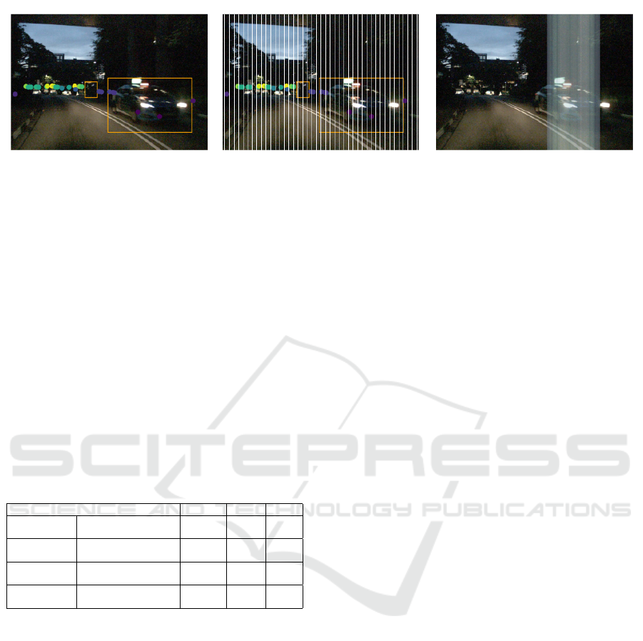
Figure 1: Preprocessing and prediction of the radar network. On the left we see the radar points projected to the front view

camera image. The center image is divided into a certain number of slices N

from which we generate the input matrix for the

training of the CNN. The right hand image corresponds to the output of the radar network.

promote automated driving. This section brieﬂy de-

scribes the characteristics of the three most used sen-

sors for the perception of the environment for auto-

mated driving, i.e., camera, radar and lidar, includ-

ing their advantages and disadvantages. Camera sen-

sors take two-dimensional images of light by electri-

cal means. They are accurate in measuring edges,

contour, texture and coloring. Furthermore they are

easily integrated into the design of a modern vehicle.

However, 3D localization from images is challeng-

ing and weather-related visual impairment can lead to

higher uncertainties in object detections (Wang et al.,

2020).

Table 1: Overview of the advantages and disadvantages of

the most common sensors for autonomous driving(Phillips,

2020).

Speciﬁcations Camera Radar Lidar

Distance

Range ++ +++ +++

Resolution ++ +++ ++

Angle

Range +++ ++ +++

Resolution +++ + ++

Classiﬁcation

Velocity Resolution + +++ ++

Object Categorization +++ + ++

Environment

Night Time + +++ +++

Rainy/Cloudy Weather + +++ ++

+ = Good, ++ = Better, +++ = Best

Radar sensors use radio waves to determine the range,

angle and relative velocity of objects. Long-range

radar sensors have a high range capability up to

200 − 250m (John and Mita, 2019; Schneider, 2005;

de Ponte M

uller, 2017) and are cheaper than Lidar

sensors (Aldrich and Wickramarathne, 2018). Com-

pared to cameras, radar sensors are less affected by

environmental conditions and pollution (Aldrich and

Wickramarathne, 2018; Fritsche et al., 2016; de Ponte

uller, 2017). On the other hand, radar data is sparse

and does not delineate the shape of the obstacles

(Fritsche et al., 2016; John and Mita, 2019). Lidar

sensors use a light beam, emitted from a laser, to de-

termine the distances and shapes of objects.

Lidar sensors are highly accurate in 3D localiza-

tion and surface measurements as well as a long-

range view up to 300m (Pidurkar et al., 2019). They

are expensive to buy and bad weather conditions like

rain, fog or dust reduce the performance (Aldrich and

Wickramarathne, 2018; de Ponte M

uller, 2017).

Each sensor has its advantages and disadvantages

(summarized in Table 1), so that a sensor fusion with

at least two sensors makes sense in order to provide a

better safety standard.

3 OBJECT DETECTION VIA

RADAR

In this section we introduce the 1D segmentation net-

work that we equip for detecting vehicles. First we

explain the pre-processing method, then we describe

the network architecture, the loss function and the net-

work output.

3.1 Preprocessing

In a global 3D coordinate system, the radar data is sit-

uated in a 2D horizontal plane. Hence, before train-

ing a neural network, we pre-process the radar data

for two reasons. First of all, in order to simplify the

fusion after processing each sensor with a neural net-

work separately, we project the given radar data into

the same 2D perspective as given by the front view

camera. Secondly, one can observe that after this

projection, the remaining section of the radar sensor

modality is close to 1D. Figure 1 depicts radar points

projected into the front view camera image. Darker

colors indicate closer objects and brighter colors indi-

cate more distant objects. Consequently, we build and

train a neural network to perform a 1D segmentation.

To be more speciﬁc, we pre-process the ground

truth for training the radar network as illustrated in

Figure 2. That is, we divide the given front view im-

age into a chosen number N

of slices and generate an

occupancy array of length N

. The ith entry of this ar-

ray is equal to 1 if there is a ground truth object inter-

YOdar: Uncertainty-based Sensor Fusion for Vehicle Detection with Camera and Radar Sensors

179

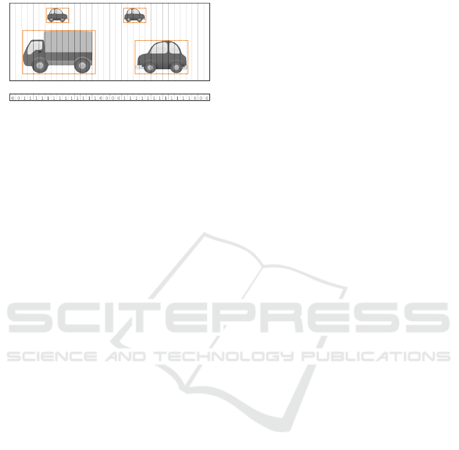
Figure 2: Ground truth vector for radar data. Every slice

that overlaps with a bounding box in the front view camera

image obtains the value 1, otherwise 0.

secting with the ith slice of the image and 0 else. This

ground truth construction deﬁnes the desired predic-

tion for the radar network.

The radar data is pre-processed similarly to the

ground truth as we aim at providing the neural net-

work with an input tensor of size N

× N

where

denotes the number of considered time steps and

denotes the number of features. By assigning radar

points to image slices we can drop the x-coordinate

(which is implied by the array index up to an quanti-

zation error). For each slice i = 1, ...,N

which con-

tains at least one radar point we store the following

features in the input matrix: y-coordinates (indi-

cating the distance of the reﬂection point), the height

coordinate with respect to the front view image that

the radar point obtains by projection into the image

plane as well as the relative lateral and the longitudi-

nal velocity.

3.2 Network Architecture

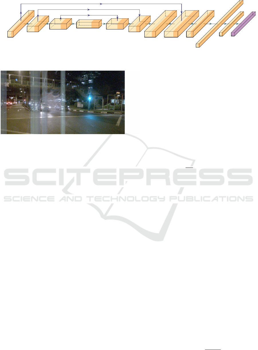
The network architecture for the radar network is

based on a FCN-8-network (Long et al., 2015) and

is depicted in Figure 3. The hidden layers consist of

three convolution blocks, three deconvolution blocks

followed by a concatenate layer, a fourth convolution

block, a ﬂatten layer and one fully-connected block.

Finally, the network contains a sigmoid layer from

which we get in [0,1]. Each convolution and deconvo-

lution block includes a (de-)convolution layer, a batch

normalization and a leaky ReLU as activation func-

tion, respectively. The convolution blocks capture

context information while losing spatial information

whereas the deconvolution blocks restore these spa-

tial information. Using bypasses, context information

can be linked with spatial information. Furthermore,

each fully connected block consists of a dense layer

followed by a leaky ReLU activation function (except

for the ﬁnal layer where we use a sigmoid activation

function).

3.3 Loss Function

Let D = {(r

(i)

) : i = 1,. . . ,n} denote a dataset

of tuples containing radar data r

(i)

∈ R

×N

and

ground truth t

(i)

∈ {0, 1}

. The radar network g pro-

vides an array of estimated probabilities indicating

whether a given slice s is occupied or not. We de-

note y

(i)

= g(r

(i)

). For training the neural network

we use the binary cross-entropy for each array entry

s = 1, . .. , N

, i.e., for a single data sample (r

(i)

)

we have

`(t

(i)

) = −αt

(i)

log(y

(i)

) − (1 −t

(i)

)log(1 − y

(i)

)

(1)

where α is a tunable parameter. We introduced this

parameter in order to account for the imbalance of ze-

ros and ones in the ground truth. When training with

stochastic batch gradient descent, the loss function is

summed over all s = 1, . . ., N

and then the mean is

computed over all indices i in the batch.

3.4 Output

The predictions of the radar network result in a vector

consisting of values in [0, 1] that estimate the proba-

bility of occupancy. Neighboring slices whose pre-

dicted probabilities are above a certain threshold T

are recognized as one coherent object, also called

slice bundle. Figure 4 shows for example an image

with four slice bundles. The more a slice bundle ﬁlls

in a bounding box, the higher the 1D IoU gets.

4 OBJECT DETECTION VIA

SENSOR FUSION

After describing the object detection method using

radar sensor data in the previous section, this sec-

tion deals with the image detection method and the

fusion of both methods. Various object detection net-

works have been developed in recent years, whereby

the YOLOv3 network has become a very good choice

when fast and accurate real-time detection is de-

sired (Redmon and Farhadi, 2018; Benjdira et al.,

2019). It has been observed that YOLOv3 works

very well under good weather and visibility condi-

tions but has problems with object recognition in bad

visibility like hazy weather (Tumas et al., 2020; Li

et al., 2020) or darkness, like Xiao et al. have investi-

gated for object detection with RFB-Net (Xiao et al.,

2020). In our experiments, we focus on object detec-

tion by camera and radar at night. To this end, we ﬁrst

use each method separately in order to connect both

outputs with gradient boosting (Friedman, 2002), see

ICAART 2021 - 13th International Conference on Agents and Artiﬁcial Intelligence

180

160

Input

Conv 1

Conv 2

128

Conv 3

Deconv 1

Deconv 2

160

Deconv 3

160

Concatenate

160

Conv 4

5760

Flatten

160

Sigmoid

Figure 3: CNN architecture of our custom FCN-8 inspired radar network.

Figure 4: Image of a radar detection example with four pre-

dicted slice bundles.

Figure 5. Similarly to (Rottmann et al., 2020) we de-

rive metrics from each CNN output and pass them

through a gradient boosting classiﬁer to increase the

number of detected vehicles. The data and metrics

used for the classiﬁer are explained in Section 5. The

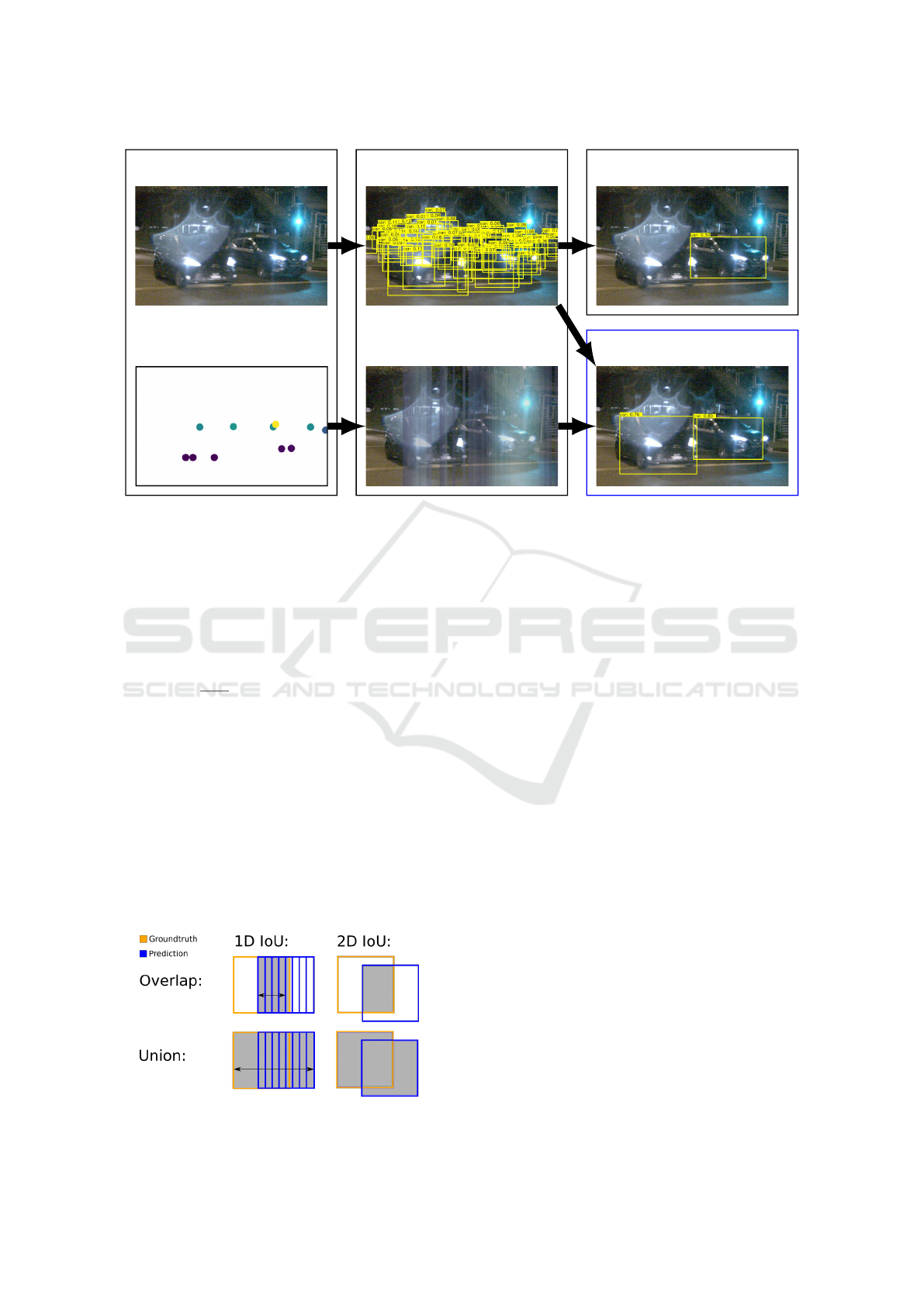
YOLOv3 threshold T

for vehicle detection is set to a

low value such that we get a higher number of bound-

ing box predictions. From the many predicted bound-

ing boxes, gradient boosting select those boxes that

are likely to contain an object according to the output

of both networks. On the one hand, the radar sensor

should detect vehicles not recognized by the YOLOv3

network. On the other hand, gradient boosting should

support the decision making process by additional in-

formation in case the YOLOv3 network is uncertain.

5 FUSION METRICS AND

METHODS

The fusion method that we introduce in this section is

of generic nature. Therefore, we denote by f the an

arbitrary camera network and by g a 1D segmentation

radar network. Given an input scene (x, r), we obtain

two network outputs, one for the image input x, one

for the radar input r. Each prediction obtained by f

consists of a set B = {b

,. . . ,b

} containing k boxes

where k depends on x. Each box b

is identiﬁed with

a tuple β

that contains an objectness score value z

, a

probability f (v|x, b

) that the box b

contains a vehicle

v, a center point with its x-coordinate c

∈ R and y-

coordinate c

∈ R as well as width w

∈ R and height

∈ R of the box, i.e.,

= (z

, f (v|x, b

),c

). (2)

For the radar network g we obtain a 1D output of

probabilities, g

(v|r) for each of the slices s = 1, .. . , n,

that this slice s belongs to a vehicle v, recall Fig-

ure 2. As depicted in Figure 1 we identify slices s

and bounding boxes b

. In order to aggregate slices

s from the radar network over bounding boxes b

ob-

tained by the camera network, let S

denote the set of

all slices s that intersect with the box b

. We denote

∑

s∈S

(v|r) (3)

the average probability of observing a vehicle in the

box b

according to the radar network’s probabilities.

The standard deviation corresponding to Equation (3)

is termed σ

. As a set of metrics, by which we com-

pute a fused prediction, we consider

(x, r) = (β

,µ

,σ

) (4)

where A

= w

· h

denotes the size of the box b

. In

summary, we use these nine metrics M

(x, r) for all

scenes (x,r) and boxes b

that are visible with respect

to the front view camera.

To perform the fusion of the camera based net-

work prediction and the radar based network predic-

tion we proceed in two steps. First we compute the

ground truth which states for each box predicted by

the camera network whether it is a true positive (TP)

or a false positive (FP). Afterwards we train a model

to discriminate by means of M

whether b

is a TP or

an FP.

More precisely, for the sake of computing ground

truth, we deﬁne TP and FP in the given context as

follows: For a predicted box b

and a ground truth

box a, which has the biggest intersection |a∩ b

| of all

ground truth boxes of the same class, the intersection

over union is deﬁned as follows:

IoU(b

) = max

|a ∩ b

|a ∪ b

. (5)

YOdar: Uncertainty-based Sensor Fusion for Vehicle Detection with Camera and Radar Sensors

181

CNN-Input CNN-Output

Prediction by YOLOv3

Prediction by fusion

Figure 5: Illustration of our YOdar method. In the top branch, the YOLOv3 produces many candidate bounding boxes, but

after score thresholding and non maximum suppression, only one of both cars is detected. By lowering the object detection

threshold and fusing the obtained boxes with the radar prediction, both cars are detected by YOdar as shown in the bottom

right panel.

Oftentimes we omit the argument b

if it is clear from

the context. Given a chosen threshold T ∈ [0, 1) we

deﬁne that b

is a TP if IoU(b

) > T and an FP if

IoU(b

) ≤ T . For the sake of completeness, we de-

ﬁne that a false negative is a ground truth box a that

fulﬁlls max

|a∩b

|a∪b

≤ T . Note that in the latter def-

inition, the ground truth element is ﬁxed while the

left hand side of this expression is maximized over all

predicted boxes. After computing the ground truths,

i.e., whether a box b

predicted by the camera net-

work yields a TP or an FP, we train a model. The

gathered metrics M

yield a structured dataset where

the columns are given by the different metrics and the

rows are given by all predicted boxes b

for each in-

put scene (x,r). By means of this dataset and the cor-

responding TP/FP annotation, we train a classiﬁer to

predict whether a box predicted by the camera net-

work is a TP or an FP.

Figure 6: IoU calculation for 1D and 2D bounding boxes.

The IoU can be calculated in different dimensions

D = 1,2. In this work the 1D IoU is used for the

radar network. As soon as a low threshold T

has been

reached, a predicted object is considered as TP, other-

wise as FP. The 2D IoU is used for the YOLOv3 net-

work, analogously we speak of TP and FP according

to a threshold T

. An illustration is given in Figure 6.

The mean average precision (mAP) is a popular metric

used to measure the performance of models. The mAP

is calculated by taking the average precision (area un-

der precision as a function of recall, a.k.a. precision

recall curve) over one class.

6 NUMERICAL EXPERIMENTS

As explained in detail in the previous section, we use

a custom FCN-8-like network for processing the radar

data from the nuScenes dataset (Caesar et al., 2020).

It contains urban driving situations in Boston and Sin-

gapore. The dataset has a high variability of scenes,

i.e., different locations, weather conditions, daytime,

recorded with left- or right-hand trafﬁc. In total, the

dataset contains 1,000 scenes, each of 20 seconds

duration and each frame is fully annotated with 3D

bounding boxes. The vehicle used, a Renault Zoe,

was set up with 6 cameras at 12Hz capture frequency,

5 long-range radar sensors (FMCW) with 13Hz cap-

ture frequency, 1 spinning lidar with 20Hz capture

ICAART 2021 - 13th International Conference on Agents and Artiﬁcial Intelligence

182

frequency, 1 global positioning system module (GPS)

and 1 inertial measurement unit (IMU). Each scene is

divided into several time frames for which each sen-

sor provides a suitable signal.

For our experiments, the YOLOv3 network was

pretrained with day images from the COCO dataset

(Lin et al., 2014) and afterwards with 249 randomly

selected scenes from the nuScenes dataset containing

10,000 images with different weather conditions and

times of day. Furthermore we have trained a CNN

with radar data from the nuScenes dataset to detect

vehicles. 743 of the scenes (29,853 frames) were used

as training data, 82 scenes (3,289 frames) as valida-

tion data and 25 scenes (1,006 frames) as test data, see

Table 2. For the test set, we consider exclusively all

frames recorded at night that are not part of the train-

ing data in order to create a perception-wise challeng-

ing test situation. For the training and validation sets

we used a natural split of day and night scenes pre-

deﬁned by the frequencies in the nuScenes dataset.

Due to the resolution of the radar data, we focus on

the category vehicle in our evaluation. This includes

the semantic categories car, bus, truck, bicycle, mo-

torcycle and construction vehicle.

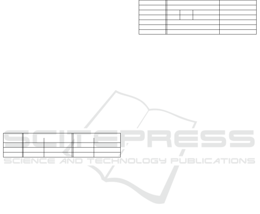
Table 2: Data used for training, validation and testing.

splitting

number of images/frames night images/frames [%]

YOLOv3 Radar YOLOv3 Radar

train 10,000 29,853 7.08 9.04

val 3,289 3,289 8.57 8.57

test 1,006 1,006 100 100

6.1 Training

As input, the radar network obtains a tensor with the

dimensions 160 × 3 × 4 that contains for each of the

160 considered slices the current frame (i.e., the cur-

rent time step) and two previous frames. Each frame

contains four features, i.e., x-, and y-coordinates, lat-

eral and longitudinal velocity. From the radar data we

removed all ground truth bounding boxes that do not

contain any radar points with valid velocity vectors.

The radar network is implemented in Keras (Chol-

let, 2015) with TensorFlow (Abadi et al., 2016) back-

end. Training on one NVIDIA Quattro GPU P6000

takes 229 seconds training time. The network struc-

ture is shown in Figure 3 and the training parameters

are shown in Table 3. We have trained the neural net-

work three times with three different learning rates,

i.e., the ﬁrst 20 epochs with a learning rate of 10

−3

, 10

epochs with 10

−4

and 10 epochs with 10

−5

. The net-

works output vector has the same dimension (160×1)

as the ground truth vector, where each entry contains

a probability value, whether there is a vehicle in the

respective area or not. If the probability value of a sin-

gle slice is equal or higher than the threshold T

= 0.5,

then the network predicts a vehicle. The higher the

probability value, the brighter the slice is displayed in

Figure 1.

Table 3: Training Parameters.

Parameter Radar YOLOv3

Batchsize 128 6

Learning rate 10

−3

−4

−5

−4

- 10

−6

Epochs 20 10 10 100

Weight decay 3 · 10

−4

variable

Loss function modiﬁed binary-crossentropy binary-crossentropy

Optimizer Adam Adam

The YOLOv3 network was trained with 10,000 im-

ages consisting of different scenes. Therefore we con-

verted the 3D bounding boxes in the nuScenes dataset

into 2D bounding ones. To this end, we chose the

smallest 2D bounding box that contains the front and

rear surfaces of the 3D bounding box in the given ego

car view. YOLOv3 is implemented in the Python-

Framework Tensor-Flow (Abadi et al., 2016). Train-

ing with the same GPU as used for the custom radar

network takes 50,32 hours training time. The training

parameters are stated in Table 3.

6.2 Evaluation

All results in this section are averaged over 3 ex-

periments to obtain a better statistical validity. Fig-

ure 7 shows absolute numbers of recognized objects

(IoU ≥ 0.5 with the ground truth) at night for each of

the networks (Radar and YOLOv3) standalone as well

as for our uncertainty-based fusion approach (YO-

dar). The numbers are broken down corresponding

to distance intervals along the horizontal axis. The

lavender bar (in the background) displays the num-

bers of vehicles in the ground truth for the given dis-

tance interval. The blue bar states the numbers of ob-

jects recognized by the radar network. The perfor-

mance of the radar network is low, only a small per-

centage of objects are found. After 20 meters, the per-

formance decreases with growing distance. The poor

recognition of objects from radar can be explained by

the small number of points provided for each frame.

In addition, relative velocities are used for training,

which means that mainly moving objects can be rec-

ognized and stationary or parked vehicles remain un-

detected. The orange bar shows a signiﬁcant increase

of objects recognized by the YOLOv3 network com-

pared to the radar network. Although mainly closer

objects are recognized, there remain difﬁculties in ob-

ject recognition with more distant objects. The green

bar shows the objects recognized by YOdar. Com-

pared to the YOLOv3 network, more vehicles are rec-

ognized for each of the given distances. In total, com-

YOdar: Uncertainty-based Sensor Fusion for Vehicle Detection with Camera and Radar Sensors

183

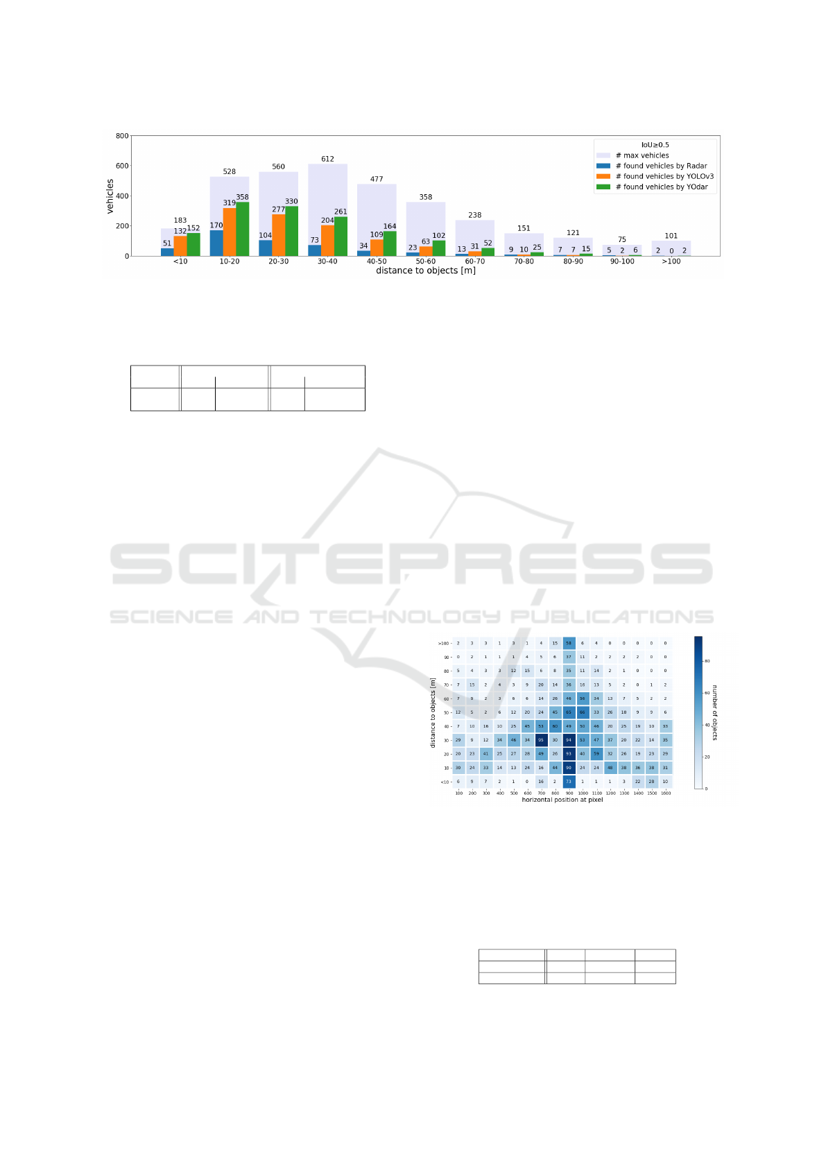
Figure 7: Vehicles recognized at night with consideration of the respective distance from the ego car. An object is considered

as detected when it has an IoU ≥ 0.5 with the ground truth. These are average values from three test runs.

Table 4: Comparison of the number of false positives for

YOLOv3 and YOdar at a common level of false positives.

Network unchanged output TP level adjustment

TP FP TP FP

YOLOv3 1,154 98 1,478 1,024

YOdar 1,467 449 1,467 449

pared to the YOLOv3 network, the sensor fusion ap-

proach recognizes 313 vehicles more (which amounts

to an increase of 9.20 percent points).

So far, we have seen that we recognize more ob-

jects with the YOdar approach than with YOLOv3 or

our radar network separately. However, the increased

sensitivity also yields some additional FPs. In order

to compare the number of FPs for YOLOv3 and YO-

dar, we adjust the sensitivity of the YOLOv3 network

by lowering the threshold T

such that the TP level for

YOLOv3 is roughly equal to the TP level of YOdar.

The resulting number of FPs is given in Table 4. In-

deed, YOdar generates 575 less FP predictions than

YOLOv3 for a common TP level, on which we let

YOdar operate in our tests.

Digging deeper into the discussed results, we

now break down the distance intervals along the dis-

tance radii. Figure 8 states the absolute numbers of

objects broken down by distance (vertical axis) and

the pixel intervals of width 100 of the input image

with a total width of 1600 pixels (horizontal axis).

More precisely, each interval denoted by i on the hor-

izontal axis represents the pixels (row, column) with

column ∈ [i − 99, i]. A ground truth object is a mem-

ber of such an interval, if the center of the box is con-

tained in the respective interval and has the respective

distance from the ego car. Thus, this can be viewed

as a spatial distribution of the ground truth where the

center of the bottom row is the area closest to the ego

car. The majority of the objects is located in the inter-

vals given by i = 500, . . . , 1,200.

Figure 9 shows the relative amount of objects

recognized by the YOLOv3 network. It shows that

mainly objects closer to the ego car and straight ahead

are recognized, while objects farther away or located

on the very left or very right end of the image re-

main often unrecognized. Figure 10 states in abso-

lute numbers how many additional objects are recog-

nized in each particular area when using YOdar in-

stead of YOLO. The increase is clear and also mostly

in the relevant areas close to the ego car and straight

ahead. This is in line with the idea of focusing with

the radar on objects in motion (by considering ob-

jects that carry velocities). These results show that

an uncertainty-based fusion approach like YOdar is

indeed able to increase the performance signiﬁcantly.

This ﬁnding is also conﬁrmed by the mAP and ac-

curacy values stated in Table 5. While YOLOv3

achieves 31.36% mAP, Yodar achieves 39.40% which

is also close to state of the art deep learning based fu-

sion results for the nuScenes dataset with the natural

split of day and night scenes as reported in (Nobis

et al., 2019).

Figure 8: Ground truth heat map displaying the spatial dis-

tribution of the test data, broken down by distance (verti-

cal axis) and the pixel intervals of width 100 of the front

view input image with a total width of 1600 pixels (hori-

zontal axis). More precisely, each intervals denoted by i on

the horizontal axis represents the pixels (row, column) with

column ∈ [i − 99, i].

Table 5: Accuracies and mAP scores of all three networks.

Radar YOLOv3 YOdar

Accuracy [%] 14.42 33.90 43.10

mAP [%] 7.93 31.36 39.40

ICAART 2021 - 13th International Conference on Agents and Artiﬁcial Intelligence

184

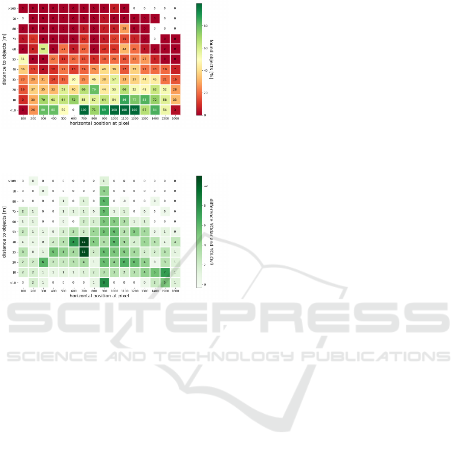
Figure 9: Relative amount of objects recognized by the

YOLOv3 network evaluated on the test data. The under-

lying geometry is the same as in Figure 8.

Figure 10: Number of objects recognized by YOdar minus

the number of objects recognized YOLOv3. The underlying

geometry is the same as in Figure 8.

7 CONCLUSION AND OUTLOOK

In this paper we have introduced the method YOdar

which detects vehicles with camera and radar sen-

sors. With this uncertainty-based sensor fusion ap-

proach the camera and radar data are ﬁrst processed

individually. Each branch detects objects, the cam-

era branch uses a YOLOv3 network trained with day

and night scenes and the radar branch uses a custom-

based radar network. The outputs of every branch are

aggregated and then passed through a post process-

ing classiﬁer that again learns the same vehicle de-

tection task. Compared to the YOLOv3 network, the

YOdar fusion method detects at night a signiﬁcant ad-

ditional amount of vehicles in total. While YOLOv3

achieves 31.36% mAP, YOdar achieves 39.40% mAP

which is also close to state of the art deep learning

based fusion results for the nuScenes dataset with the

natural split of day and night scenes. In future work,

additional sensors will be added for training and eval-

uation, since this approach uses only the front cam-

era and the front radar sensor. Furthermore, we plan

to optimize the radar network such that more objects

can be detected by YOdar. Moreover, we plan to ex-

tend this approach also the detection of pedestrians as

more dense radar data becomes available.

ACKNOWLEDGEMENTS

K.K. acknowledges ﬁnancial support through the re-

search consortium bergisch.smart.mobility funded by

the ministry for economy, innovation, digitalization

and energy (MWIDE) of the state North Rhine West-

phalia under the grant-no. DMR-1-2.

REFERENCES

Abadi, M., Agarwal, A., Barham, P., et al. (2016). Ten-

sorFlow: Large-Scale Machine Learning on Hetero-

geneous Systems. CoRR, abs/1603.04467.

Aldrich, R. and Wickramarathne, T. (2018). Low-cost radar

for object tracking in autonomous driving: A data-

fusion approach. In 2018 IEEE 87th Vehicular Tech-

nology Conference (VTC Spring), pages 1–5.

Benjdira, B., Khursheed, T., Koubaa, A., et al. (2019). Car

Detection using Unmanned Aerial Vehicles: Compar-

ison between Faster R-CNN and YOLOv3. In 2019

1st International Conference on Unmanned Vehicle

Systems-Oman (UVS), pages 1–6.

Caesar, H., Bankiti, V., Lang, A. H., et al. (2020). nuscenes:

A multimodal dataset for autonomous driving. In 2020

IEEE/CVF Conference on Computer Vision and Pat-

tern Recognition, CVPR 2020, Seattle, WA, USA, June

13-19, 2020, pages 11618–11628. IEEE.

Chan, R., Rottmann, M., H

uger, F., Schlicht, P., and

Gottschalk, H. (2020). Controlled False Negative Re-

duction of Minority Classes in Semantic Segmenta-

tion. In 2020 IEEE International Joint Conference on

Neural Networks (IJCNN).

Chollet, F. (2015). Keras - Deep learning library. Available:

https://github.com/keras-team/keras.

de Ponte M

uller, F. (2017). Survey on Ranging Sensors

and Cooperative Techniques for Relative Positioning

of Vehicles. Sensors, 17.

Dosovitskiy, A., Ros, G., Codevilla, F., et al. (2017).

CARLA: an open urban driving simulator. In 1st

Annual Conference on Robot Learning, CoRL 2017,

Mountain View, California, USA, November 13-15,

2017, Proceedings, volume 78 of Proceedings of Ma-

chine Learning Research, pages 1–16. PMLR.

Friedman, J. H. (2002). Stochastic gradient boosting. Com-

putational Statistics & Data Analysis, 38(4):367–378.

Fritsche, P., Kueppers, S., Briese, G., et al. (2016). Radar

and lidar sensorfusion in low visibility environments.

In Proceedings of the 13th International Conference

on Informatics in Control, Automation and Robotics

(ICINCO 2016) - Volume 2, Lisbon, Portugal, July 29-

31, 2016, pages 30–36. SciTePress.

Gu, S., Zhang, Y., Tang, J., et al. (2019). Road Detection

through CRF based LiDAR-Camera Fusion. In 2019

YOdar: Uncertainty-based Sensor Fusion for Vehicle Detection with Camera and Radar Sensors

185

International Conference on Robotics and Automation

(ICRA), pages 3832–3838.

Hansen, M. K. and Underwood, J. P. (2017). Multi-modal

obstacle detection in unstructured environments with

conditional random ﬁelds. CoRR, abs/1706.02908.

John, V. and Mita, S. (2019). RVNet: Deep Sensor Fusion

of Monocular Camera and Radar for Image-Based Ob-

stacle Detection in Challenging Environments. In Lec-

ture Notes in Computer Science (including subseries

Lecture Notes in Artiﬁcial Intelligence and Lecture

Notes in Bioinformatics), volume 11854 LNCS, pages

351–364.

Li, G., Yang, Y., and Qu, X. (2020). Deep Learn-

ing Approaches on Pedestrian Detection in Hazy

Weather. IEEE Transactions on Industrial Electron-

ics, 67(10):8889–8899.

Lin, T., Maire, M., Belongie, S. J., et al. (2014). Mi-

crosoft COCO: common objects in context. In Com-

puter Vision - ECCV 2014 - 13th European Confer-

ence, Zurich, Switzerland, September 6-12, 2014, Pro-

ceedings, Part V, volume 8693 of Lecture Notes in

Computer Science, pages 740–755. Springer.

Liu, Z., Yu, S., Wang, X., and Zheng, N. (2017). Detecting

drivable area for self-driving cars: An unsupervised

approach. CoRR, abs/1705.00451.

Long, J., Shelhamer, E., and Darrell, T. (2015). Fully Con-

volutional Networks for Semantic Segmentation. In

Proceedings of the IEEE Conference on Computer Vi-

sion and Pattern Recognition (CVPR).

Maag, K., Rottmann, M., and Gottschalk, H. (2020). Time-

Dynamic Estimates of the Reliability of Deep Seman-

tic Segmentation Networks. In IEEE International

Conference on Tools with Artiﬁcial Intelligence (IC-

TAI).

Nobis, F., Geisslinger, M., Weber, M., et al. (2019). A

deep learning-based radar and camera sensor fusion

architecture for object detection. In 2019 Sensor Data

Fusion: Trends, Solutions, Applications, SDF 2019,

Bonn, Germany, October 15-17, 2019, pages 1–7.

IEEE.

Phillips, J. (2020). Achieving Safe Autonomous

Driving. Available: https://www.ni.com/de-

de/perspectives/imminent-trade-offs-for-achieving-

safe-autonomous-driving.html.

Pidurkar, A., Sadakale, R., and Prakash, A. K. (2019).

Monocular camera based computer vision system for

cost effective autonomous vehicle. In 2019 10th Inter-

national Conference on Computing, Communication

and Networking Technologies (ICCCNT), pages 1–5.

erez, R., Schubert, F., Rasshofer, R., and Biebl, E. (2019).

A machine learning joint lidar and radar classiﬁcation

system in urban automotive scenarios. Advances in

Radio Science, 17:129–136.

Redmon, J. and Farhadi, A. (2018). Yolov3: An incremental

improvement. CoRR, abs/1804.02767.

Rong, G., Shin, B. H., Tabatabaee, H., et al. (2020). LGSVL

simulator: A high ﬁdelity simulator for autonomous

driving. CoRR, abs/2005.03778.

Rottmann, M., Colling, P., Hack, T. P., Chan, R., H

uger,

F., Schlicht, P., and Gottschalk, H. (2020). Predic-

tion Error Meta Classiﬁcation in Semantic Segmenta-

tion: Detection via Aggregated Dispersion Measures

of Softmax Probabilities. In 2020 IEEE International

Joint Conference on Neural Networks (IJCNN).

Rottmann, M. and Schubert, M. (2019). Uncertainty Mea-

sures and Prediction Quality Rating for the Seman-

tic Segmentation of Nested Multi Resolution Street

Scene Images. In Proceedings of the IEEE/CVF Con-

ference on Computer Vision and Pattern Recognition

(CVPR) Workshops.

Schneider, M. (2005). Automotive radar: Status and trends.

In In Proceedings of the German Microwave Confer-

ence GeMIC 2005, pages 144–147.

Schubert, M., Kahl, K., and Rottmann, M. (2020).

Metadetect: Uncertainty quantiﬁcation and predic-

tion quality estimates for object detection. CoRR,

abs/2010.01695v2.

Silva, V. D., Roche, J., and Kondoz, A. M. (2018). Ro-

bust fusion of lidar and wide-angle camera data for

autonomous mobile robots. Sensors, 18(8):2730.

Tumas, P., Nowosielski, A., and Serackis, A. (2020). Pedes-

trian Detection in Severe Weather Conditions. IEEE

Access, 8:62775–62784.

Wang, Z., Wu, Y., and Niu, Q. (2020). Multi-sensor fu-

sion in automated driving: A survey. IEEE Access,

8:2847–2868.

Wu, T.-E., Tsai, C.-C., and Guo, J.-I. (2017). Li-

DAR/camera sensor fusion technology for pedestrian

detection. In 2017 Asia-Paciﬁc Signal and Informa-

tion Processing Association Annual Summit and Con-

ference (APSIPA ASC), pages 1675–1678.

Xiao, Y., Jiang, A., Ye, J., and Wang, M.-W. (2020). Mak-

ing of Night Vision: Object Detection Under Low-

Illumination. IEEE Access, 8:123075–123086.

ICAART 2021 - 13th International Conference on Agents and Artiﬁcial Intelligence

186