Using Geometric Graph Matching in Image Registration

Giomar O. Sequeiros Olivera

1 a

, Aura Conci

2 b

and Leandro A. F. Fernandes

2 c

Anhanguera Educacional, Niter

oi, RJ, Brazil

Institute of Computing, Fluminense Federal University, Niter

oi, RJ, Brazil

Keywords:

Image Registration, Graph Matching, Edit Distance, Infrared Images.

Abstract:

Image registration is a fundamental task in many medical applications, allowing interpreting and analyzing

images acquired using different technologies, from different viewpoints, or at different times. The image

registration task is particularly challenging when the images have little high-frequency information and when

average brightness changes over time, as is the case with infrared breast exams acquired using a dynamic

protocol. This paper presents a new method for registering these images, where each one is represented in a

compact form by a geometric graph, and the registration is done by comparing graphs. The application of the

proposed technique consists of ﬁve stages: (i) pre-process the infrared breast image; (ii) extract the internal

linear structures that characterize arteries, vascular structures, and other hot regions; (iii) create a geometric

graph to represent such structures; (iv) perform structure registration by comparing graphs; and (v) estimate

the transformation function. The Dice coefﬁcient, Jaccard index, and total overlap agreement measure are

considered to evaluate the results’ quality. The output obtained on a public database of infrared breast images

is compared against SURF interest points for image registration and a state of the art approach for infrared

breast image registration from the literature. The analyzes show that the proposed method outperforms others.

1 INTRODUCTION

Medical image processing has become a fundamen-

tal tool in healthcare, being increasingly used in tasks

such as diagnostic, treatment planning, surgeries, and

disease follow-up (Rahman, 2018). In medical image-

based applications, it is often interesting to analyze

more than one set of data simultaneously since im-

ages obtained with different acquisition technologies

may reveal complementary information about struc-

tures of interest (Balakrishnan et al., 2018). More-

over, same patient images taken at different times can

help to monitor abnormalities or assist their treatment.

In both cases, image registration (IR) is an essential

task in the processing of medical images, being cru-

cial in all applications that need to combine, compare,

or merge visual information (Brock et al., 2017; Conci

et al., 2015; Gonz

alez et al., 2018).

The IR process consists of estimating a func-

tion that allows mapping one of the images to the

other (Zitov

a and Flusser, 2003). For this purpose,

a wide variety of IR techniques can be seen in the

https://orcid.org/0000-0002-7172-6525

https://orcid.org/0000-0003-0782-2501

https://orcid.org/0000-0001-8491-793X

literature, that in general are divided into intensity-

based and feature-based methods (Zitov

a and Flusser,

2003). For the second approaches, it is necessary

to manually, semi-automatically, or automatically ex-

tract feature points from the images (Ma et al., 2016).

The manual and semi-automatic selection of feature

points are usually time-consuming and often imprac-

tical. Consequently, it is important to develop tech-

niques that allow the automatic identiﬁcation of these

points. Moreover, those techniques must be stable to

ensure consistency and reproduction of the results.

Unfortunately, the most used approaches for auto-

matic identiﬁcation of feature points in natural images

are not adequate for IR of low contrast images such as

infrared images (a.k.a. thermograms or thermal im-

ages) (Falco et al., 2020). Similarly, some approaches

use anatomical structures present in the medical im-

ages to perform the registration (Deng et al., 2010).

When applied to infrared breast images, the prob-

lem in this type of IR approach is to represent the

anatomical structures properly. In this sense, geomet-

ric graphs emerge as a powerful tool to represent ob-

jects and their spatial relationships (Garcia-Guevara

et al., 2018). Graph matching has been applied in sev-

eral domains to solve problems such as data retrieval,

Olivera, G., Conci, A. and Fernandes, L.

Using Geometric Graph Matching in Image Registration.

DOI: 10.5220/0010239200870098

In Proceedings of the 16th International Joint Conference on Computer Vision, Imaging and Computer Graphics Theory and Applications (VISIGRAPP 2021) - Volume 4: VISAPP, pages

87-98

ISBN: 978-989-758-488-6

graph classiﬁcation, pattern discovery, and structural

data characterization (Pinheiro et al., 2017) but are

still little explored for IR (Tong et al., 2017).

In this paper, we present a method for extract-

ing the location of internal linear structures from in-

frared breast images and represent them as geometric

graphs. The internal linear structures may be arteries,

vascular structures, or hot regions. We also present

an algorithm to match the graph representations of

the structures extracted from two images. The pro-

posed matching procedure is an adaptation of the edit

distance (Armiti and Gertz, 2014) that, in addition to

considering the structural relationships of a vertex and

its neighbors, uses local image descriptors around the

edge that connects two vertices to improve the match-

ing. We have applied this proposition for registering

breast examinations and have observed signiﬁcant ad-

vantages when compared it to previous techniques.

The remaining of this paper is organized as fol-

lows: Section 2 presents a literature review of related

works. The proposed approach is detailed in Sec-

tion 3. Section 4 presents the experiments and their

results. Finally, Section 5 concludes the paper and

points to directions for future exploration.

2 RELATED WORK

There are few approaches in the literature for breast

infrared IR. To the best of our knowledge, none of

them uses graph-based techniques to perform the task.

Thus, we claim that this is one of the original contri-

butions of our work. Next, we discuss some works

that extend traditional IR methods to thermograms.

Agostini et al. (2009) recorded about 500 frames

of thermal images. Prior acquisition, they glued black

and white markers of 5mm diameter on the patient’s

skin. The white markers are used for estimating

the transformations between image pairs, while the

black markers are used to measure the quality of the

method. The alignment of the set of frames is per-

formed by taking the ﬁrst image of the sequence as the

reference, being the others transformed to it. Since

the white markers guide registration, the method be-

gins with the automatic identiﬁcation of this kind of

marker. After that, each marker is manually labeled

and used to solve the linear transformation that bet-

ter explains their location in the image pair. The efﬁ-

cacy of this method is measured by the signal-to-noise

ratio (SNR). In this case, the signal analyzed along

the series is formed by the temperatures in the posi-

tions of the black markers in the ﬁrst frame, together

with the temperature of the same positions in the other

images. The noise calculated by the measurement is

characterized by the change throughout the series of

the temperature values in the observed locations.

Lee et al. (2010) also proposed the IR of infrared

images by using markers previously placed on the

patient. These markers are automatically identiﬁed

by the Harrys’ corners detection method (Harris and

Stephens, 1988). After that, the association between

markers in both images is manually set by the user.

Through these association, a transformation by Thin

Plate Spline function (Holden, 2008) is calculated and

used to align the sensitive to the reference image.

In the end, the transformation function is reﬁned by

the simplex method. In subsequent work, Lee et al.

(2012) used the Harris corner coefﬁcient to detect fea-

ture points from heat patterns on the thermal images.

Registration is made by taking the ﬁrst image as a ref-

erence and estimating transformations that explain the

location of the feature points on other image of the set.

To evaluate the proposed approach, numbered mark-

ers were placed on a patient, and a sequence of ten

images of that patient was acquired. During the ac-

quisition, the patients are instructed to perform small

movements, simulating the displacements that occur

in examinations that take large time intervals.

Silva et al. (2016) used an IR process as part of

a methodology that aims to analyze thermograms us-

ing time series. In their methodology, thermograms

are sequentially acquired, forming a set of twenty im-

ages per patient. During the ﬁve minutes of acqui-

sitions, the patient performs small involuntary move-

ments for breathing. These movements lead to differ-

ences from one thermogram to another. In Silva et al.

(2016) work, the ﬁrst thermogram of the sequence

is considered the reference image, and the others are

deemed sensitive images. Thus, for the examination

of a patient, the registration process is executed nine-

teen times since the sensitive thermograms of the se-

quence must be registered to the ﬁrst one. Silva et al.

(2016) technique uses Mutual Information (MI) as a

global measure of similarity of pixel intensities to es-

timate translation, rotation, and scale transformations

between the images.

Falco et al. (2020) used the same dataset of Silva

et al. (2016) for IR. All the serial thermograms of

the same patient are analyzed, creating a relationship

among them. The reference image for registration is

chosen as the one that is more similar to all the others.

Then, all the other thermograms of a patient are regis-

tered systematically, creating a new and more similar

set of thermograms. Initially, the images to be regis-

tered are classiﬁed as a reference or sensitive image.

After that, all images are processed to estimate the sil-

houette of the patient’s body. Through the silhouette,

feature points are identiﬁed. These points are used to

VISAPP 2021 - 16th International Conference on Computer Vision Theory and Applications

estimate the transformation that better explains the lo-

cation of the feature points from one image to another.

With these transformations, a new set of serial images

are created, one for each type of transformation com-

puted. Finally, the generated images are compared

with the reference image, and the set of registered im-

ages that presented the best result is chosen as the out-

put of the registration method.

It is important to note that the techniques men-

tioned above either rely on markers to perform the

registration or local information that may change

from one image to another, such as the infrared in-

tensity or the patient’s silhouette. Our approach, on

the other hand, performs the registration based on the

topological relationship between the main sources of

heat identiﬁed in the image, which are related to the

arteries, vascular structures, and other hot regions.

3 THE PROPOSED APPROACH

Our method for infrared breast IR consists of ﬁve

steps: (i) pre-process a given infrared breast image;

(ii) extract the internal linear structures; (iii) repre-

sent the internal structures using a geometric graph;

(iv) perform graph matching to register the graph of

the current image to the graph of another thermogram;

and (v) estimate the transformation for image registra-

tion. The following subsections describe these steps.

3.1 Pre-processing

Infrared images are formed by a temperature matrix

representing the thermal pixel values. By using a

min-max mapping, temperatures values may be rep-

resented in the [0, 255] range as a conventional 8-bit

grayscale image. Such an image can also be treated

as a heightmap, i.e., the gray intensity value assigned

at pixel location (x, y) also represents the distance of

displacement or elevation of a surface, with 0 (black)

representing minimum height and 255 (white) repre-

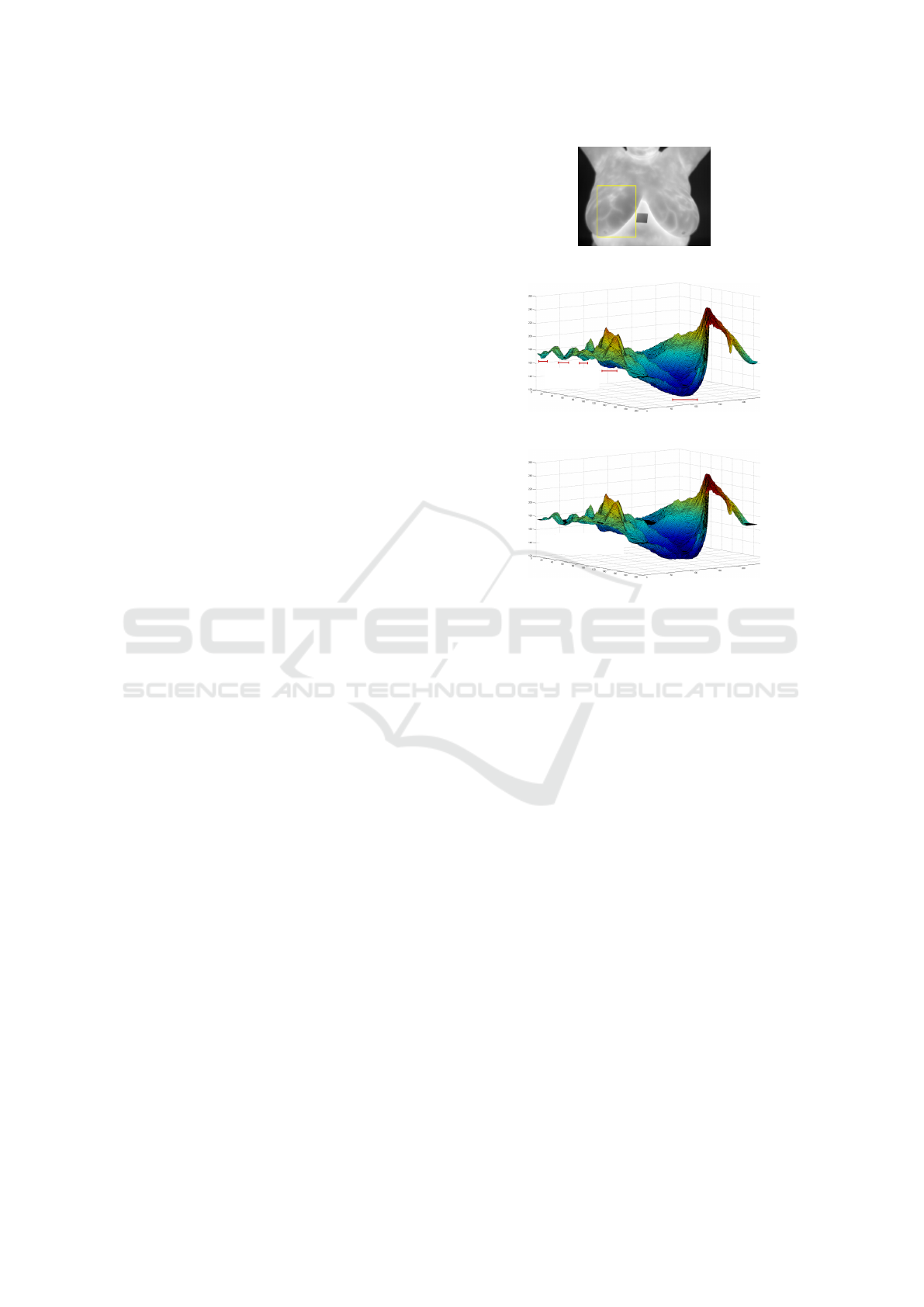
senting maximum height. Figures 1 (a) and (b) exem-

plify, respectively, an infrared breast image and the

region enclosed by the rectangle in (a) represented as

a relief. When the whole image is considered, the

highest portions of the terrain are the warmest regions

of the patient’s body, with part of the ridges indicat-

ing the location of thicker blood vessels. Global mini-

mum regions correspond to the background, i.e., areas

outside the patient’s body.

The purpose of the pre-processing step is to pre-

pare the image to facilitate the extraction of internal

linear structures in the next step. According to our

experience, global minimum and more accentuated

(a)

Local Minimum

Regions

(b)

Removal of

Local Minimum Regions

(c)

Figure 1: Three-Dimensional representation of the yellow

portion of a thermogram (a) as a height map before (b) and

after (c) applying the H-minima transform. Notice that the

relief around local minimum in (b) have changed in (c).

local minima affect the quality of the segmentation

algorithm that is used in the next step to extract in-

ternal linear structures. To solve this problem, we

apply the H-minima transform (Ismail et al., 2016)

as a pre-processing to suppresses all minima in the

grayscale image whose intensity is less than h. Fig-

ures 1 (b) and (c) illustrate the relief induced by the

thermogram before and after the application of the H-

minima transform. Through empirical experimenta-

tion, we observed that the value h = 8 meets the needs

of the proposed technique.

3.2 Extraction of Linear Structures

The input of this step is the image resulting from the

pre-processing stage. The result is a binary image

where 1-pixels represent the location of the internal

linear structures, which correspond to ridges of the

relief induced by the thermogram.

In this work, we use the watershed algorithm by

ﬂooding (Kornilov and Safonov, 2018) to achieve the

objective of the internal linear structures’ extraction

step. This algorithm simulates relief ﬂooding from

water sources located at local minimum. When the

Using Geometric Graph Matching in Image Registration

(a) (b) (c)

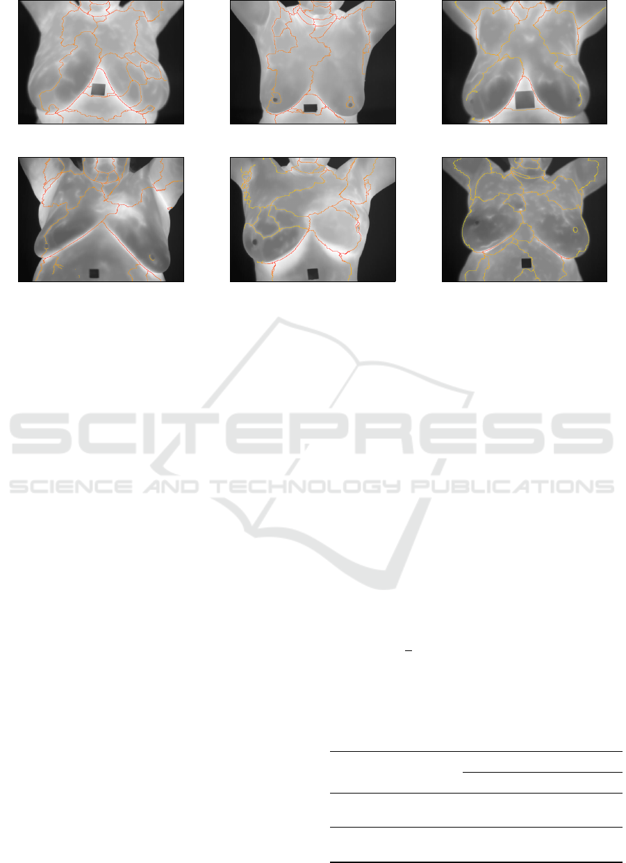
Figure 2: From left to right: (a) the original thermogram; (b) internal structures for (a); and (c) internal structures for the

image resulting from the H-minima transform of (a).

water rises, retention basins are created. At the end

of the ﬂooding process, neighboring basins deﬁne the

watershed lines. Figure 2 (b) shows the watershed

of the non pre-processed gray-level image in Fig-

ure 2 (a). As it is possible to observe, many lines

were deﬁned as the internal linear structures because

many retention basins were created. Figure 2 (c)

shows the result of the watershed segmentation ap-

plied to the version of Figure 2 (a) pre-processed by

the H-minima transform. This result presents a much

cleaner set of linear features.

The binary image produced by the watershed al-

gorithm is subsequently processed by the thinning

procedure described by Zhang and Suen (1984). The

objective is to obtain a binary image with structures

having the thickness of one pixel.

3.3 Linear Structure Representation

Once the internal structure is extracted, it must be

turned into a geometric graph. For this, we start with

an 8-connected neighborhood representation of the

binary image obtained in the previous step.

Let G = (V, E) be an undirected graph, where V

is the set of vertices and E the set of edges. The ver-

tices v ∈V correspond to the 1-pixels of the given bi-

nary image, and the 8-connected neighborhood of 1-

pixels deﬁnes the edges e = (v

, v

) ∈ E for any pair

of neighbor vertices v

, v

∈V . The graph is geomet-

ric because vertices carry the (x, y) pixels’ location,

and edges’ weight is given by the Euclidean distance

between the pixels of the vertices that deﬁne them.

Thus, the weight of an edge can be equal to 1 or

√

One problem that arises in representing the inter-

nal linear structures using G is the creation of too

many vertices, which can compromise the perfor-

mance of matching algorithms (Zheng et al., 2013).

To mitigate this issue, we create the geometric graph

= (V

, E

) from the graph G = (V, E). Here,

⊆V is the new set of vertices formed by endpoints,

corners, and junction points of the linear structures

in the given binary image. The new set of edges

⊆V

×V

allows connecting vertices in V

consid-

ering the shortest paths in V . Additionally, the new

graph is enhanced with the inclusion of features at the

vertices and edges. Below we describe the processes

for obtaining the new sets of vertices and edges, and

how to extract the features to be assigned to elements

of the new graph.

Determination of the New Set of Vertices. The

candidate vertices for graph G

= (V

, E

) must sat-

isfy one of the three rules below:

1. v ∈V is an endpoint, i.e., degree(v) = 1;

2. v ∈V is a corner, i.e., degree(v) = 2 and the ver-

tex v and its direct neighbors are not collinear;

3. v ∈V is a junction point, i.e., degree(v) ≥ 3;

were degree(v) is the number of vertices directly con-

nected to v. To avoid creating many close vertices in

, we only include in V

the candidate vertices that

do not have another candidate vertex within a radius

bounded by the threshold d. In our experiments, we

observed that the value d = 20 meets the needs of the

proposed technique for the image database we have

using. This value must be adjusted for other databases

regarding the resolution of the input thermograms and

the patient’s distance to the camera.

Determination of the New Set of Edges. The set

of edges E becomes obsolete when the new collec-

tion V

of vertices is deﬁned as a subset of V . There-

fore, we need to build E

to reconnect the vertices that

were included in the graph G

. We use the graph G in

this process to not lose the overall structure of the lin-

ear features depicted in the input binary image. More

speciﬁcally, we create edges e

= (v

, v

) ∈ E

using

the Dijkstra algorithm to determine the shortest path

between v

and v

in the original graph G. An edge is

created whenever there is no vertex in V

positioned

between vertices v

and v

in such path.

VISAPP 2021 - 16th International Conference on Computer Vision Theory and Applications

Figure 3: Example of visual feature extraction.

Feature Extraction. The purpose of this step is to

create spatial features vectors and visual feature vec-

tors for the elements in the geometric graph G

Spatial features are associated with vertices. For

a given vertex v

∈V

, its spatial features are encoded

by a cyclic string of tuples, F = [ f

, f

, ··· , f

], where

n = degree(v

) and f

is a tuple (|e

|, < e

i−1

). Here,

| represents the length of the edge e

= (v

, v

where v

is the neighbor vertex reached from v

through e

, and < e

i−1

denotes the angle between

the edges e

and e

i−1

in counterclockwise order.

Visual feature vectors are created to encode visual

information around the graph edges. For this purpose,

we use Histogram of Oriented Gradients (HOG) fea-

tures (Dalal and Triggs, 2005), generally applied in

pattern recognition and image processing to detect or

recognize objects. In the present case, the objects

represent variations of intensities nearby the thicker

blood vessels in the original infrared breast image.

We compute one HOG feature from the 8 ×8 grid

placed at the center point of each edge of the graph G

The cells in this grid are grouped into 2 ×2 blocks,

and the orientation of the gradients of each pixel of

the image is transformed in such a way that they are

mapped to the [−180

◦

, 180

◦

) range, with a 40

◦

in-

terval, i.e., the orientations assume values in the dis-

crete set {−180

◦

, −140

◦

, −100

◦

, −60

◦

, −20

◦

,20

◦

,100

◦

,140

◦

}. After this process, the magnitude of

each pixel is used as a weighting factor for calculat-

ing the average orientation of each cell. Finally, each

block is represented by a histogram of average orien-

tations. Histograms of 9 bins are created, and since

we have 4 blocks, the whole feature vector will have

size 36. Figure 3 illustrates the computation of the

HOG features.

3.4 Graph Matching

This step aims to perform the comparison of graphs

and F

representing, respectively, the reference and

the sensitive images, to obtain the best correspon-

dence between their vertices. From this correspon-

dence, it will be possible to estimate the transforma-

tion that will allow registering the thermograms.

Algorithm 1 estimates the resulting matching ma-

trix. We use the Hungarian method (Riesen et al.,

2018) to ﬁnd the best matching between the vertices

of G

and F

from the matrix M, whose entry M

i, j

represents the cost of transforming the information

related to the i-th vertex v

∈ G

into the information

assigned to the j-th vertex u

∈ F

(see Algorithm 2).

The vertex transformation cost is computed by

Algorithm 3 as the vertex edit distance (Armiti and

Gertz, 2014). Editing distance is a measure of similar-

ity and represents a powerful approach within error-

tolerant methods for correspondence between graphs.

This distance involves basic operations such as re-

moving, adding, or replacing vertices and edges. This

distance is calculated using dynamic programming

with complexity O(nm

), where n = degree(v

) and

m = degree(u

) (Armiti and Gertz, 2014). We imple-

ment the substitution, insertion, and removal opera-

tions applied in the edit distance algorithms follow-

ing Armiti and Gertz (2014).

The following are the edit operations on the edges:

substitution, insertion, and removal. Given two ver-

tices v and u, let be the edge e

the neighbor of v and

the edge e

the neighbor of u. The substitution cost

between two edges is deﬁned as:

γ(e

→ e

) = d

, e

) + d

, e

), (1)

where d

, e

) returns the Euclidean distance be-

Algorithm 1: Geometric graph matching.

1 SetAlFnt

Input: Graphs G

= (V

, E

) and F

= (U

, D

)

Output: The matching matrix

2 foreach v

∈V

3 i ← the index of v

;

4 foreach u

∈U

5 j ← the index of u

;

6 M

i, j

← computeMinimalDistance(v

, u

);

7 return HungarianMethod(M);

Using Geometric Graph Matching in Image Registration

tween the visual features of the edges e

and e

that

were extracted by using HOG features. Similarly,

, e

) returns the spatial distance based on angles

and length of the edges:

, e

) =

(

c(e

, e

) , for |θ

−θ

| ≤ π,

c(e

, e

) + 2 max{l

, l

} , otherwise,

(2)

where

c(e

, e

) =

+ l

−2l

cos(|θ

−θ

|), (3)

and θ

is the angle between an edge and the previous

one and l

is the length of the edge.

The cost of substitution is deﬁned as the distance

required so that the neighboring vertex of the edge

is aligned with the neighboring vertex of the edge

, which can be seen as the polar distance between

them. The cost for insertion and removal operations

are deﬁned by:

γ(λ → e

) = γ(e

→ λ) =

(

c(e

) + d

) , for θ

≤ π,

c(e

) + 2l

+ d

) , otherwise,

(4)

where

c(e

) =

+ l

i−1

−2l

i−1

cos(|θ

|). (5)

3.5 Image Registration

In this work, we assume that the transformation used

to register the sensitive image to the reference im-

age is a planar homography. The result of the pre-

vious step is the best match between the vertices of

two geometric graphs representing thermograms. In

some cases, incorrect matches (outliers) may occur,

introducing errors in the homography that would be

estimated if all corresponding vertices were consid-

ered. Consequently, the image registration step uses

the RANSAC algorithm (Fischler and Bolles, 1981)

to remove outliers and estimate the best homogra-

phy between the actual corresponding vertices (in-

liers). The resulting transformation function serves

to change the sensitive image, making it more similar

to the reference one. For this, it is necessary to use in-

terpolation techniques that map the continuous values

of the transformation function into discrete values of

the image representation domain (Pan et al., 2012).

4 EXPERIMENTS AND RESULTS

Following Falco et al. (2020) and Silva et al. (2015), a

sample from the DMR-IR database (Silva et al., 2016)

Algorithm 2: Compute minimal distance.

1 SetAlFnt

Input: Vertices v

and u

Output: minimal distance

2 word1 ← spatial and visual features from v

;

3 word2 ← spatial and visual features from u

;

4 n ← degree(v

);

5 m ← degree(u

);

6 if n <m then

7 swap(word 1,word2);

8 minimalDistance ← ∞;

9 for i ← 1 to m do

10 word2 ←rotate(word 2);

11 distance ← editDistance(word1,word2);

12 if distance >minimalDistance then

13 minimalDistance ← distance;

14 return minimalDistance;

Algorithm 3: Edit distance.

1 SetAlFnt

Input: Spatial and visual features

word1andword2

Output: The edit distance stored in D

n+1,m+1

2 n ← length(word1);

3 m ← length(word2);

4 for i ← 1 to n do

5 D

i,1

← i;

6 for j ← 1 to m do

7 D

1, j

← j;

8 for i ← 1 to n do

9 c1 ← the i-th entry of word1;

10 for j ← 1 to m do

11 c2 ← the j-th entry of word2;

12 if c1 = c2 then

13 D

i+1, j+1

← D

i, j

;

14 else

15 D

i+1, j+1

← min{

i, j

+ SubstitutionCost(c1, c2),

i, j+1

+InsertRemoveCost(c1, c2),

i+1, j

+InsertRemoveCost(c1, c2)};

16 return D

n+1,m+1

;

was used to carry out the experiments and to validate

the proposed approach. From these, 11 healthy pa-

tients and 12 with disease diagnoses were selected

due their diversity of body shapes. Each one has a set

of 20 frontal images captured every 15 seconds during

5 minutes according to a protocol proposed by Silva

et al. (2016). This time is long enough for the patient

to perform involuntary movements in such a way that

becomes necessary the IR before analysis.

We have considered the ﬁrst thermogram of each

patient as the reference image, and the remaining 19

thermograms have been considered the sensitive im-

ages that will be registered to the ﬁrst one. Due to

VISAPP 2021 - 16th International Conference on Computer Vision Theory and Applications

(a) (b) (c)

(d) (e) (f)

Figure 4: Examples of structures extracted from thermograms of healthy patients (a)-(c), and from thermograms of patients

diagnosed with a disease in the breast (d)-(f).

the non-deterministic nature of the RANSAC algo-

rithm, we have performed the registration of each

pair of images ten times. We have considered the

average transformation as the expected transforma-

tion. By doing so, we avoid small variations from

one registration to another in the same pair of im-

ages. Thus, having 23 patients with 20 images each,

19 ×10 = 190 RANSAC evaluations were performed

per patient, leading to a total of 4,370 registrations.

For simplicity, through this section, the patients

are identiﬁed by the numbering P1, P2, . . . , P23.

Patients P1 to P11 correspond to those with healthy

breasts, while patients P12 to P23 present some breast

disease diagnoses. Figure 4 shows the linear struc-

tures (orange lines) extracted from some of such im-

ages, of which Figures 4 (a)-(c) are from healthy pa-

tients, and Figures 4 (d)-(f) are from breast disease

patients. It is important to mention that each im-

age shown in Figure 4 represents the ﬁrst in a se-

ries of 20 images acquired by using a dynamic pro-

tocol proposed by Silva et al. (2016). The diagnoses

were obtained through other exams (mammography

or biopsy) and the visual differences are not necessar-

ily evident enough to distinguish between healthy and

diseased patients by analysing just one thermogram.

An example of visual differences between healthy and

diseased patients is the presence of asymmetries heat

distribution in the left and right breast. Figure 5 shows

the geometric graphs deﬁned from the linear struc-

tures presented in Figure 4.

Next, we discuss the complexity of the geometric

graphs constructed using the proposed approach and

two other suggested solutions, the performance of the

proposed technique in the registration of images of

each patient, and its performance comparison to other

IR techniques.

Number of Vertices. Table 1 compares the aver-

age number and the standard deviation (SD) of the

number of vertices in three types of geometric graphs

computed per patient’s condition on images of the

dataset used in our experiments. Recall that we are

considering 23 patients, with 20 images each, mak-

ing 460 geometric graphs, where 220 are related to

healthy patients, and 240 are related to patients with

some breast disease.

In Table 1, the graph type N-8 considers the bi-

nary image representing the thermogram’s watershed

structure as a graph where each 1-pixel is a vertex.

The 8-connectivity between pixels deﬁnes edges of

length 1 or

√

2. In graph type Harris, the Harris cor-

ner detector (Harris and Stephens, 1988) was applied

to the watershed image to identify the graph’s ver-

Table 1: Average and standard deviation (SD) of the number

of vertices per patient’s condition.

Condition Measure

Graph Type

N-8 Harris Ours

Healthy

Average 3319.55 422.73 173.27

SD 477.67 58.22 25.02

With

Disease

Average 4039.25 523.00 209.75

SD 825.86 104.71 43.45

Using Geometric Graph Matching in Image Registration

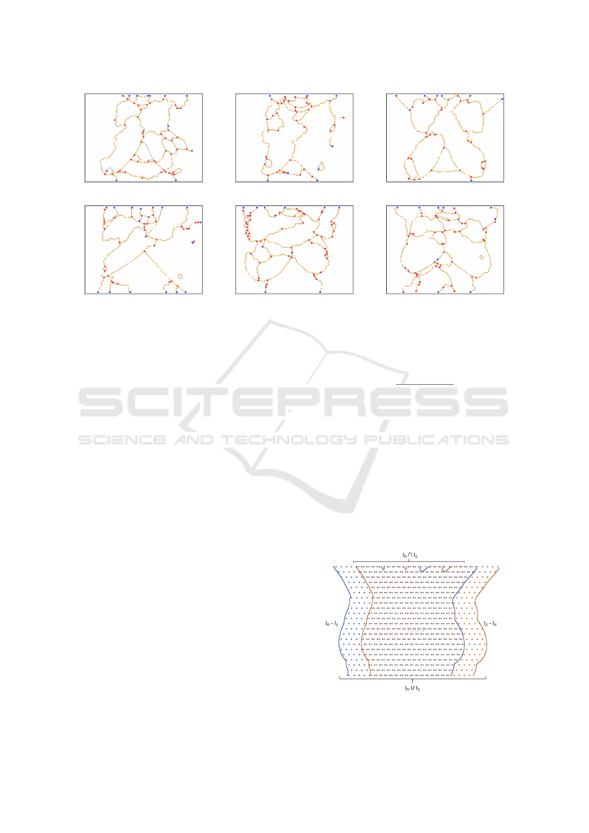
(a) (b) (c)

(d) (e) (f)

Figure 5: Geometric graphs computed from the thermograms presented in Figure 4. Blue, orange and red vertices correspond

to vertices created from, respectively, endpoints, corners, and junction points.

tices as the detected points of interest. Notice that

the average number and the SD of vertices produced

by the proposed approach is much smaller than the

values resulting from graphs of type N-8 and Harris.

It is necessary to have about 173 vertices on average

to represent the internal structures of the thermogram

with healthy diagnosis and 210 vertices for patients

with some disease. The importance of having a small

number of vertices to represent the structures prop-

erly resides in the fact that graph matching algorithms

are NP-complete (Riesen et al., 2018). Thus, be able

to describe the structures present in the thermograms

with less information is a desirable property of the

proposed approach. Such a property allows obtaining

a considerable computational performance gain in the

execution of graph matching algorithms.

Performance of the Registration. Table 2 presents

the performance of the proposed graph-based IR

approach per patient. The analysis considers the

mean Dice coefﬁcient (Dice, 1945), mean Jaccard in-

dex (Jaccard, 1912), and mean Total Overlap Agree-

ment (TOA) measure (Klein et al., 2009) achieved

before and after registration. Table 2 also presents

the number of times in which the evaluation measure

gets improved after IR. These values have been high-

lighted for convenience. Similarly, Table 3 shows the

standard deviation per patient before and after regis-

tration. In this case, the increments of standard devi-

ation after registration are highlighted, and they indi-

cate greater dispersion in relation to the mean.

The Dice coefﬁcient is deﬁned as:

Dice =

2N (I

∩I

)

N (I

) + N (I

)

, (6)

where I

and I

are the binary representation of, re-

spectively, the reference and sensitive images. These

binary images are considered as sets whose elements

are the pixels that form the patient’s body. Here, N (S )

is the number of elements in the set S. Thus, it gives

the area of the objects formed by 1-pixels in the given

image, that can be seen in Figure 6. To that extent,

Dice coefﬁcient equal to 1 means the total overlap, the

greater similarity between the images, while 0 means

no overlap.

The Jaccard index represents the percentage of

Figure 6: Comparison between reference image I

and sen-

sitive image I

VISAPP 2021 - 16th International Conference on Computer Vision Theory and Applications

Table 2: Mean performance results per patient before and after using the proposed IR technique.

Healthy

Patient

Dice Jaccard TOA

Before After Before After Before After

P1 0.97275 0.98511 0.98617 0.99249 0.98528 0.98879

P2 0.88114 0.92625 0.93563 0.96160 0.94110 0.94836

P3 0.92052 0.95638 0.95836 0.97766 0.96167 0.98204

P4 0.91520 0.91190 0.95534 0.95379 0.96774 0.93614

P5 0.97410 0.98584 0.98684 0.99285 0.98311 0.99066

P6 0.96601 0.97545 0.98269 0.98755 0.98795 0.98357

P7 0.90388 0.96251 0.94897 0.98082 0.94532 0.97394

P8 0.94357 0.97285 0.97094 0.98592 0.96495 0.97987

P9 0.94280 0.97477 0.97034 0.98720 0.96922 0.98075

P10 0.95459 0.97377 0.97674 0.98670 0.96572 0.98209

P11 0.97641 0.96841 0.98805 0.98393 0.98979 0.97793

Improved/Subjects 9/11 9/11 8/11

Patient

with Disease

Dice Jaccard TOA

Before After Before After Before After

P12 0.97569 0.97634 0.98768 0.98770 0.98209 0.98256

P13 0.91645 0.94692 0.95610 0.97266 0.95920 0.95609

P14 0.93368 0.95948 0.96537 0.97926 0.96919 0.98325

P15 0.97468 0.96117 0.98717 0.98008 0.98828 0.97179

P16 0.97230 0.95491 0.98593 0.97682 0.98993 0.97251

P17 0.97370 0.97787 0.98665 0.98879 0.97607 0.98210

P18 0.96957 0.96970 0.98454 0.98456 0.98576 0.98474

P19 0.93046 0.92758 0.96385 0.96236 0.96490 0.94261

P20 0.97691 0.96566 0.98831 0.98251 0.99157 0.97271

P21 0.94886 0.95382 0.97348 0.97582 0.97446 0.96801

P22 0.96275 0.96974 0.98098 0.98461 0.97918 0.97741

P23 0.97168 0.97826 0.98561 0.98900 0.98915 0.98338

Improved/Subjects 8/12 8/12 3/12

Total Improved/Subjects 17/23 17/23 11/23

overlap of two sets in relation to their union:

Jaccard =

N (I

∩I

)

N (I

∪I

)

. (7)

Like the Dice coefﬁcient, Jaccard index equal to 1

means greater similarity between the images, while

0 indicates no similarities.

The TOA measure for a given registration is:

TOA =

N (I

∩I

)

N (I

)

, (8)

whose value also range from 0 to 1.

We have used similarity measures based on bi-

nary images following works in the literature. This

allows our technique to be compared with other ap-

proaches. Besides, the intensity information on the

patient’s thermographs varies over time because of the

dynamic protocol (Silva et al., 2016). This variation

can introduce errors in the analysis when the intensi-

ties are compared directly after registration.

From Table 2, it is possible to observe that, ac-

cording to the Dice coefﬁcient and Jaccard index,

the proposed IR approach improved the registration

of images of 9 out 11 healthy patients and 8 out

12 patients with a disease. For the Dice coefﬁcient,

the evaluation measure values increased up to 0.0586

units in success cases (subject P7) and decreased up

to 0.0174 units in the other cases (subject P16). For

the Jaccard index and TOA measure, the most signif-

icant performance improvement was of 0.0166 (sub-

ject P13) and 0.0286 units (subject P7), respectively,

while the greatest deterioration in performances were

of, respectively, 0.0091 (subject P16) and 0.0316

units (subject P4). These results show that the bene-

ﬁts of the proposed technique outweigh the problems

it may introduce.

From a more detailed look at the registration re-

sults, it was observed that, in a general way, the pro-

posed method performed well, achieving IR improve-

ments in 77% of the pairs of images of healthy pa-

Using Geometric Graph Matching in Image Registration

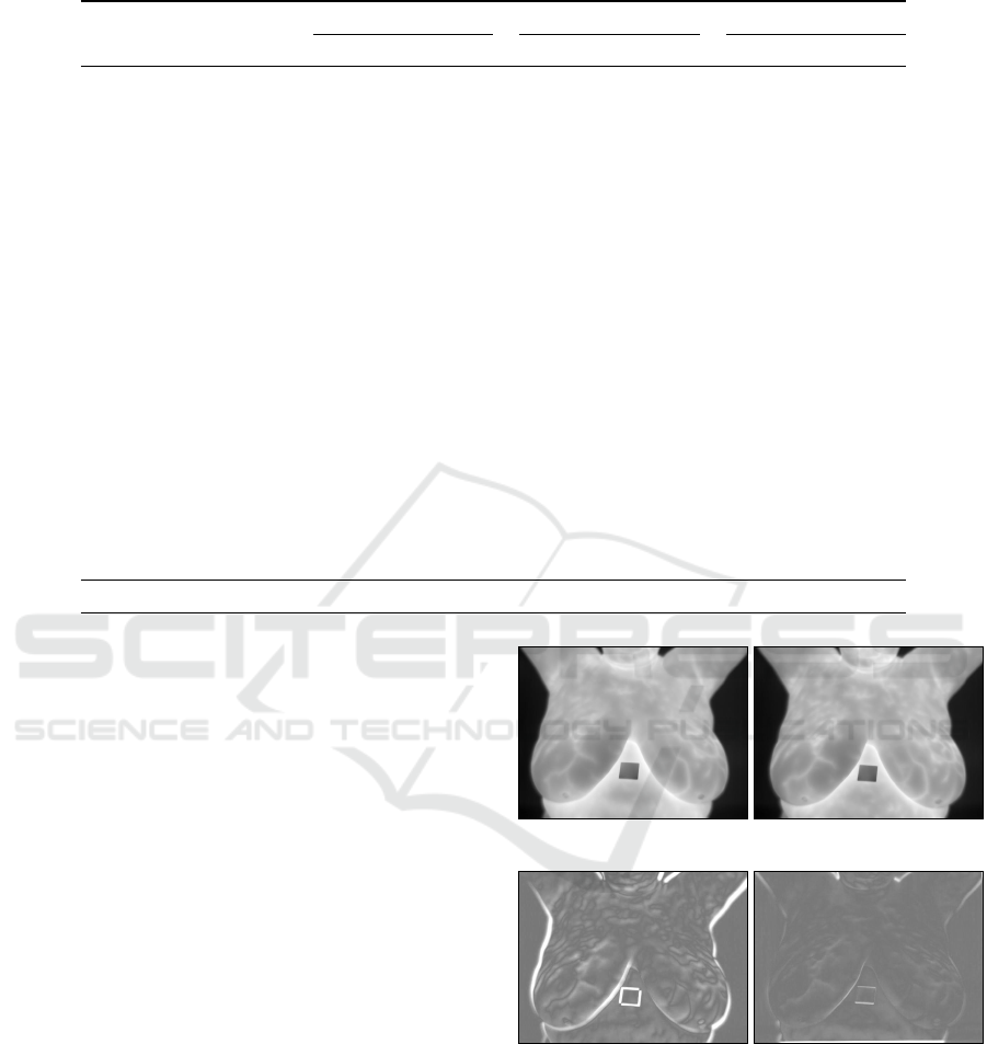
Table 3: Standard deviation performance results per patient before and after using the proposed IR technique.

Patient

Dice Jaccard TOA

Before After Before After Before After

P1 0.00654 0.00581 0.00335 0.00295 0.00356 0.00457

P2 0.06300 0.02134 0.03744 0.01144 0.04407 0.01878

P3 0.03094 0.01257 0.01684 0.00660 0.01693 0.00767

P4 0.03740 0.02177 0.02067 0.01183 0.02031 0.01820

P5 0.01336 0.00924 0.00687 0.00472 0.00900 0.00800

P6 0.00877 0.01035 0.00452 0.00531 0.00704 0.00891

P7 0.04465 0.01687 0.02453 0.00880 0.02387 0.01480

P8 0.01067 0.03501 0.00563 0.01864 0.00800 0.02189

P9 0.02912 0.01002 0.01548 0.00515 0.01553 0.00883

P10 0.01141 0.00614 0.05970 0.00315 0.00693 0.00473

P11 0.00673 0.00861 0.03440 0.00443 0.00400 0.00686

P12 0.00797 0.03590 0.00410 0.01940 0.00593 0.03573

P13 0.03378 0.01736 0.01834 0.00909 0.01549 0.01522

P14 0.03536 0.01510 0.01943 0.00795 0.02024 0.00935

P15 0.00676 0.02167 0.00346 0.01128 0.00233 0.01748

P16 0.00859 0.02164 0.00441 0.01148 0.00308 0.01165

P17 0.00904 0.00939 0.00463 0.00485 0.00889 0.00797

P18 0.00826 0.01486 0.00426 0.00776 0.00411 0.00570

P19 0.02218 0.01626 0.01194 0.00874 0.01467 0.01506

P20 0.00600 0.00853 0.00308 0.00442 0.00344 0.00757

P21 0.03275 0.04485 0.17470 0.02512 0.01858 0.02642

P22 0.01191 0.01046 0.00615 0.00537 0.00748 0.00869

P23 0.01000 0.00592 0.00517 0.00302 0.00436 0.00614

Total Improved/Subjects 14/23 16/23 10/23

tients. In the case of patients with diseases, there were

improvement in 56% of the image pairs.

Figures 7 (a) and (b) exemplify, respectively, the

reference image and 19

sensitive image for patient

P1. Figure 7 (c) shows the pixelwise difference be-

tween (a) and (b) without performing IR, while Fig-

ure 7 (d) shows the difference after performing the

proposed IR technique. In both images (c) and (d),

darker and lighter regions correspond to more signif-

icant (signed) differences. Results were mapped to

the [0, 255] range to improve visualization. A notice-

able superposition improvement can be observed after

IR, where most of the image (d) takes a medium gray

tone, which represents a difference close to zero.

Processing Time. The testbed implementation of

our approach was not tailored for performance. Even

so, it is capable of performing image registration in

less than one second on a PC with Intel Core i5 6500

CPU and 8GB of RAM.

Comparison to Other Approaches. Figure 8

shows a summary of the performance achieved by

the proposed method, the method described by Falco

et al. (2020), and the traditional use of SURF to ex-

ecute IR. As one can see, SURF performed worse,

not being competitive with either of the other two

(a) (b)

Figure 7: Example of a thermogram taken as the reference

image (a) and the 19

sensitive image (b) of a given pa-

tient. Images (c) and (d) show the normalized pixel by pixel

difference between images (a) and (b) before and after ap-

plying the proposed IR technique, respectively.

techniques. It is because SURF and related feature

extraction techniques, e.g., SIFT and ORB, require

high-frequency information to characterize textured

regions properly. By using the Dice coefﬁcient as the

VISAPP 2021 - 16th International Conference on Computer Vision Theory and Applications

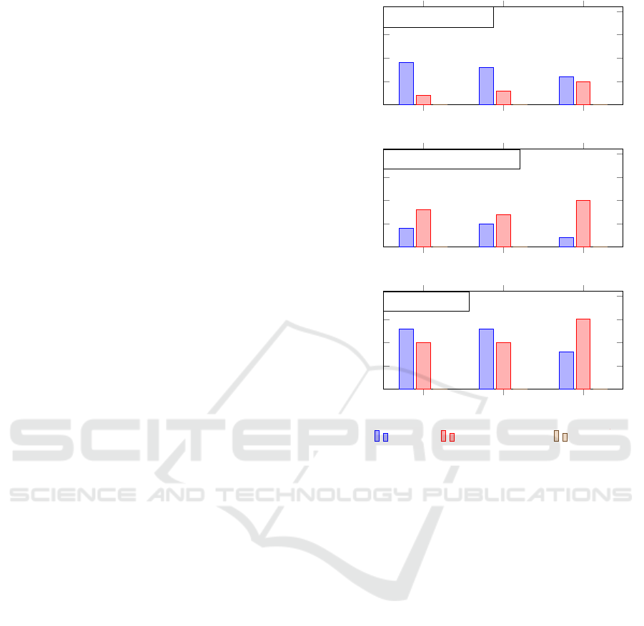
evaluation measure, our method performs better regis-

tering of healthy patients in 9 out of 11 cases, against

2 out of 11 cases where Falco’s et al. approach per-

formed better (Figure 8, a). For the Jaccard index, the

mean performance of our approach was higher for 8

against 3 subjects. The TOA measure shows a score

of 6 against 5 cases of better performance of the pro-

posed technique over Falco’s et al. approach. When

patients with a disease are considered, results show

that the Falco et al. method is slightly superior (Fig-

ure 8, b). But considering all subjects (Figure 8, c),

our approach is superior in two of the three evalua-

tion measures assumed.

5 CONCLUSIONS

This paper proposed an automatic method for infrared

breast IR by using a geometric graph matching ap-

proach. The graph that was created has a reduced

number of vertices that make it computationally ef-

ﬁcient. The execution of our registration method per-

formed well, especially in healthy patients. In these

patients, the temperature change during the dynamic

image acquisition protocol seems to be more stable.

On the other hand, in patients with breast disease,

more signiﬁcant changes were observed in the appar-

ent internal linear structures, leading to substantial

changes in the graphs’ structure and, consequently,

affecting the matching process. Nevertheless, the re-

sults presented in this paper are interesting since they

indicate that the ﬁrst technique to use graphs for in-

frared breasts IR is promising.

Several works may emerge from the proposed ap-

proach. For instance, it is possible to modify the edit

distance model to assign different weights to the in-

sert, replace, and remove operations to allow different

priorities to be set to the operations.

Another possible direction of future work is using

other types of visual features to characterize the local

information around a vertex or an edge, including the

use of features extracted by artiﬁcial neural networks.

Finally, our approach could be adapted to differ-

ent types of medical images with linear and vascular

structures such as fundus images widely used to diag-

nose ocular diseases or diseases that have global ef-

fects on the vascular system (Bhatkalkar et al., 2020).

ACKNOWLEDGEMENTS

The Brazilian research agency CAPES sponsored

Giomar O. S. Olivera. Aura Conci is par-

tially supported by MACC-INCT, CNPq (grants

Dice Jaccard TOA

0 0 0

Number o Wins

(a) Healthy Patients

Dice Jaccard TOA

0 0 0

Number o Wins

(b) Patients with Disease

Dice Jaccard TOA

13 13

10 10

0 0 0

Number o Wins

Proposed Falco et al. (2020) SURF

Figure 8: Summary of the comparison of results for healthy

patients, patients with breast disease, and the total number

of patients using the proposed approach, the IR technique

described by Falco et al. (2020), and SURF.

402988/2016-7 and 305416/2018-9), and FAPERJ

(project SIADE-2 and 210.019/2020). Leandro A.

F. Fernandes is partially supported by the Brazilian

research agencies CNPq (grant 424507/2018-8) and

FAPERJ (grant E-26/202.718/2018).

REFERENCES

Agostini, V., Knaﬂitz, M., and Molinari, F. (2009). Motion

artifact reduction in breast dynamic infrared imaging.

IEEE Trans. Biomedical Engineering, 56(3):903–906.

Armiti, A. and Gertz, M. (2014). Vertex similarity - a basic

framework for matching geometric graphs. In Pro-

ceedings of the LWA, pages 111–122.

Balakrishnan, G., Zhao, A., Sabuncu, M. R., Guttag, J., and

Dalca, A. V. (2018). An unsupervised learning model

for deformable medical image registration. In Pro-

ceedings of the IEEE Conference on Computer Vision

and Pattern Recognition, pages 9252–9260.

Bhatkalkar, B., Joshi, A., Prabhu, S., and Bhandary, S.

(2020). Automated fundus image quality assessment

Using Geometric Graph Matching in Image Registration

and segmentation of optic disc using convolutional

neural networks. International Journal of Electrical

& Computer Engineering, 10:2088–8708.

Brock, K. K., Mutic, S., McNutt, T. R., and H. Li and, M.

L. K. (2017). Use of image registration and fusion

algorithms and techniques in radiotherapy: report of

the AAPM Radiation Therapy Committee Task Group

No. 132. Medical Physics, 44(7):43–76.

Conci, A., Galv

ao, S. S., Sequeiros, G. O., Saade, D. C., and

MacHenry, T. A. (2015). A new measure for compar-

ing biomedical regions of interest in segmentation of

digital images. Discrete Appl. Math., 197:103–113.

Dalal, N. and Triggs, B. (2005). Histograms of oriented

gradients for human detection. In Proceedings of

the IEEE Conference on Computer Vision and Pattern

Recognition, pages 886–893.

Deng, K., Tian, J., Zheng, J., Zhang, X., Dai, X., and Xu,

M. (2010). Retinal fundus image registration via vas-

cular structure graph matching. International Journal

of Biomedical Imaging, 2010:906067.

Dice, L. R. (1945). Measures of the amount of ecologic

association between species. Ecology, 26(3):297–302.

Falco, A. D., Galv

ao, S., and Conci, A. (2020). A non lin-

ear registration without the use of the brightness con-

stancy hypothesis. In Proc. Intern. Conference Sys-

tems, Signals and Image Processing, pages 27–32.

Fischler, M. A. and Bolles, R. C. (1981). Random sample

consensus: a paradigm for model ﬁtting with appli-

cations to image analysis and automated cartography.

Communications of the ACM, 24(6):381–395.

Garcia-Guevara, J., Peterlik, I., Berger, M. O., and Cotin, S.

(2018). Biomechanics-based graph matching for aug-

mented CT-CBCT. International Journal of Computer

Assisted Radiology and Surgery, 13(6):805–813.

Gonz

alez, J. R., Pupo, Y., Hernandez, M., Conci, A.,

Machenry, T., and Fiirst, W. (2018). On image reg-

istration for study of thyroid disorders by infrared ex-

ams. In Proc. Intern. Conf. Image Proc., Computer

Vision, & Pattern Recognition, pages 151–158.

Harris, C. and Stephens, M. (1988). A combined corner

and edge detector. In Proceedings of the Alvey Vision

Conference, pages 147–151.

Holden, M. (2008). A review of geometric transformations

for nonrigid body registration. IEEE Transactions on

Medical Imaging, 27(1):111–28.

Ismail, N. H. F., Zaini, T. R. M., Jaafar, M., and Pin,

N. C. (2016). H-minima transform for segmentation

of structured surface. In Proceedings of the MATEC

Web of Conferences, page 25.

Jaccard, P. (1912). The distribution of the ﬂora in the alpine

zone. New Phytologist, 11(2):37–50.

Klein, A., Andersson, J., Ardekani, B. A., Ashburner, J.,

Avants, B., Chiang, M. C., Christensen, G. E., Collins,

D. L., Gee, J., Hellier, P., Song, J. H., Jenkinson,

M., Lepage, C., Rueckert, D., Thompson, P., Ver-

cauteren, T., Woods, R. P., Mann, J. J., and Parsey,

R. V. (2009). Evaluation of 14 nonlinear deformation

algorithms applied to human brain MRI registration.

NeuroImage, 49(3):786–802.

Kornilov, A. and Safonov, I. (2018). An overview of wa-

tershed algorithm implementations in open source li-

braries. Journal of Imaging, 4(10):123.

Lee, C., Chang, Z., Lee, W., Lee, S., Chen, C., Chang,

Y., and Huang, C. (2012). Longitudinal registration

for breast IR image without markers. In Proceed-

ings of the International Conference on Quantitative

InfraRed Thermography.

Lee, C., Chuang, C. C., Chang, Z. W., Lee, W. J., Lee,

C. Y., C, S., Lee, Huang, C. S., Chang, Y. C., and

Chen, C. M. (2010). Quantitative dual-spectrum in-

frared approach for breast cancer detection. In Pro-

ceedings of the International Conference on Quanti-

tative InfraRed Thermography.

Ma, J., Zhao, J., and Yuille, A. L. (2016). Non-rigid point

set registration by preserving global and local struc-

tures. IEEE Trans. Image Processing, 25(1):53–64.

Pan, M. S., Yang, X. L., and Tang, J. T. (2012). Research

on interpolation methods in medical image process-

ing. Journal of Medical Systems, 36(2):777–807.

Pinheiro, M. A., Kybic, J., and Fua, P. (2017). Geometric

graph matching using Monte Carlo tree search. IEEE

Transactions on Pattern Analysis and Machine Intel-

ligence, 39(11):2171–2185.

Rahman, M. M. (2018). Literature-based biomedical image

retrieval with multimodal query expansion and data

fusion based on relevance feedback (RF). In Proc. In-

tern. Conference Image Processing, Computer Vision,

& Pattern Recognition, pages 103–107.

Riesen, K., Fischer, A., and Bunke, H. (2018). On the

impact of using utilities rather than costs for graph

matching. Neural Processing Letters, 48(2):691–707.

Silva, L. F., Santos, A. A., Bravo, R. S., Silva, A. C.,

Muchaluat-Saade, D. C., and Conci, A. (2016). Hy-

brid analysis for indicating patients with breast cancer

using temperature time series. Computer Methods and

Programs in Biomedicine, 130:142–153.

Silva, L. F., Sequeiros, G., Santos, M. L., Fontes, C. A. P.,

Muchaluat-Saade, D., and Conci, A. (2015). Ther-

mal signal analysis for breast cancer risk veriﬁca-

tion. Studies in Health Technology and Informatics,

216:746–50.

Tong, Y., Udupa, J. K., Ciesielski, K. C., Wu, C., Mc-

Donough, J. M., Mong, D. A., and Campbell Jr, R. M.

(2017). Retrospective 4D MR image construction

from free-breathing slice acquisitions: a novel graph-

based approach. Medical Image Analysis, 35:345–

359.

Zhang, T. Y. and Suen, C. Y. (1984). A fast parallel algo-

rithm for thinning digital patterns. Communications

of the ACM, 27(3):236–239.

Zheng, W., Zou, L., Lian, X., Wang, D., and Zhao, D.

(2013). Graph similarity search with edit distance

constraint in large graph databases. In Proceedings

of the ACM International Conference on Information

& Knowledge Management, pages 1595–1600.

Zitov

a, B. and Flusser, J. (2003). Image registration

methods: a survey. Image and Vision Computing,

21(11):977–1000.

VISAPP 2021 - 16th International Conference on Computer Vision Theory and Applications