
Storage Fees in a Container Yard with Multiple Customer Types
Yahel Giat
a
Department of Industrial Engineering, Jerusalem College of Technology, HaVaad HaLeumi 21, Jerusalem, Israel
Keywords:
Container Yard, Marine Shipment, Pricing, Poisson Arrivals, TEU.
Abstract:
We consider a small container storage yard that is located in the outskirts of a marine shipping port. Customers
are classified according to the number of storage space they need. The yard has a limited number of storage
spots, and serves customers only if there is sufficient space to fulfill their needs. We define the yard’s state
space and derive its steady-state probability matrix for Markovian arrivals and service times. We consider the
profit function of two services that the yard offers its customers. In the first, storage fees are independent of
the storage duration and in the second they are proportional to it. We show when these pricing schemes are
equivalent and demonstrate numerically how profits depend on customer arrivals rates and yard size.
1 INTRODUCTION
In the shipping industry, container yards may have to
store containers for some time before they are trans-
ported to their next destination. We consider a small
container yard located near a marine port that pro-
vides two service schemes. In the first, the yard
owner manages the entire container-shipping process
and therefore the client is unmindful and not respon-
sible for the storage time in the yard, whereas in the
second scheme, it is the customer that orders the entry
and exit of the container from the yard. Accordingly,
in the first service scheme, customer fees are indepen-
dent of the storage duration (“one-time fee”). In con-
trast, under the second scheme, storage fees are pro-
portional to the storage duration (“proportional fee”).
Customers’ arrivals to the yard is assumed to fol-
low a Poisson process. In the simplest setting, each
customer requires storage for a single container, if
such is available. If there is no vacant spot then the
customer is rejected and receives service elsewhere
(i.e., no backlogging). The general setting extends to
multiple customer types. Here, the arrivals of type-k
customers follow a Poisson process with rate λ
k
and
they require k units of storage space for a time that is
exponentially distributed with mean µ
k
.
Since the two services are offered to customers,
the yard owner is interested to determine whether one
service is more profitable than the other. In other
words, given a proportional and one-time fees, which
a
https://orcid.org/0000-0001-7296-8852
service provides a greater profit to the owner? Alter-
natively, we wish to find whether it is possible to set
specific fees for each service such that their pricing
schemes are equivalent. Furthermore, when the yard
owner has the ability to change the yard’s size (for ex-
ample, through leasing to and from neighboring lots),
then the question rises what is the optimal lot size?
To address these questions we describe the state
space of the yard and the probability of the yard to be
in each state. We then show that if for each customer
type the proportional fee is set to be equal to the one-
time fee multiplied by the expected service time, then
the two pricing schemes are equivalent.
We use a numerical illustration to show proper-
ties of the profit function, in particular to demon-
strate optimal yard size and the effects of customer ar-
rivals rate on the profit function. While the motivation
of this paper are container yard operations, we note
that the model can be applied to many other settings.
For example, parking lots serve vehicles of varying
sizes (e.g., mini cars; passenger cars; vans; minibuses;
buses). Another notable example is the telecommu-
nication industry, when customers with larger band-
width demands require more servers than those with
smaller bandwidth needs (Moscholios et al., 2016).
Managers of such systems may benefit from applying
our model to their particular settings.
Giat, Y.
Storage Fees in a Container Yard with Multiple Customer Types.
DOI: 10.5220/0010239001770184
In Proceedings of the 10th International Conference on Operations Research and Enterprise Systems (ICORES 2021), pages 177-184
ISBN: 978-989-758-485-5
Copyright
c
2021 by SCITEPRESS – Science and Technology Publications, Lda. All rights reserved
177

2 LITERATURE REVIEW
Queueing systems in which a customer may require
more than one server arise naturally in many cases.
The queueing system that is most related to our model
are the M/M/m queues. The notation M/M/m de-
scribes a queuing systems with Markovian arrival
times, Markovian service time with m servers. Green
(1980) and Green (1981) studies an M/M/m version
assuming that the servers assigned to the same cus-
tomer do not end service simultaneously, that is, these
servers become available independently. They derive
analytic expressions for the distribution of the wait-
ing time in the queue and the distribution of the num-
ber of busy servers. A similar model is developed
in Federgruen and Green (1984) assuming that each
server has a general service time distribution. They
use an approximation for the queue-length distribu-
tion. In contrast to these papers, in Fletcher et al.
(1986) the servers become available simultaneously.
Hassin et al. (2015) consider an M/M/K/K system
with a fixed budget for servers. The system owner’s
problem is choosing the price, and selecting the num-
ber and quality of the servers, in order to maximize
profits, subject to a budget constraint. In their model,
however, there is only one customer type. In contrast,
our model is similar to Kaufman (1981) and allows
for multiple customer types where each type differs
in the number of servers that it requires.
In 1968, the International Organization for Stan-
dardization (ISO) introduced the ISO 668 standard,
detailing classification, dimensions and ratings for
freight containers (ISO, 2020). While standard ISO
shipping containers have an assortment of size the
vast majority come in one of two lengths twenty feet
(6.06m) and forty feet (12.2m). For example, as of
2012, 84 percent of the global feet containers were
either twenty or forty feel long (Notteboom et al.,
2020). The twenty foot container is typically used
as the unit measure, also called Twenty Equivalent
Unit Container (TEU). Accordingly, the forty feet
container is sometimes called a two TEU container or
a Forty Equivalent Unit Container (FEU). The TEU
measure is used mainly in the marine shipping indus-
try, with ship sizes measured according to their TEU
capacity.
Pricing schemes for container storage service has
been explored in various settings. Yu et al. (2011)
focuses on the pricing of incoming containers. Our
model is more related to Woo et al. (2016) who an-
alyzes pricing storage of outgoing containers. Their
pricing structure is nonlinear where there is a limited
free storage time that is followed by a per day stor-
age fee. Our study emphasizes a single aspect of the
container freight shipping cycle, whereas other stud-
ies focus on other steps in the process. For exam-
ple, Zhang et al. (2014) optimize the repositioning of
empty containers, Chan et al. (2019) attempt to fore-
cast ports’ container throughput, and Dong and Song
(2012) consider the optimal leasing of the containers
themselves.
Container storage is similar to autonomous vehi-
cle storage and retrieval systems. These systems share
two critical features with the container storage prob-
lem. First, they park vehicles with varying sizes and
therefore may demand a different number of storage
units. Second, vehicles can be easily moved around
so that vacant storage units can be located adjacently
to accommodate large vehicles that require multiple
units. See Marchet et al. (2012) for an analysis of
such a system. Similarly, our model can be applied
to the management of recharging docks in electric ve-
hicle charging stations (Dreyfuss and Giat, 2017). In
this setting recharging docks are the system’s servers
and vehicles with larger batteries may require more
recharging docks than smaller batteries.
3 A CONTAINER YARD
We begin with description of a simple yard model in
which there are only two types of customers. In Sec-
tion 3.2 we show that these results can be extended to
any number of customer types.
3.1 Two Customer Types
A yard owner provides short-term container storage.
The yard has S storage spots and customers arrive
with a single container that is either a TEU or FEU.
TEU’s require a single storage spot and FEU’s re-
quire two spots. It is relatively easy to move con-
tainers around (“remarshalling”), and therefore any
two available spots can be made to store an FEU. We
assume no backlogging and therefore if there is no
room to store a container, then the customer stores
their container elsewhere.
Customers’ arrivals and storage times are indepen-
dent of each other. We assume that the arrivals of the
FEU’s and TEU’s follow a Poisson process with rates
λ
F
and λ
T
, respectively. Storage times of containers
in the yard are exponential with means µ
F
and µ
T
for
the FEU’s and the TEU’s, respectively.
The yard’s current state is the number of FEU’s
and TEU’s that are currently stored in it. Let (i, j) de-
note the state in which there are i FEU’s and j TEU’s
stored in the yard and let K denote the state space of
ICORES 2021 - 10th International Conference on Operations Research and Enterprise Systems
178

6
-
0
1
2
S−1
2
S−3
2
S−5
2
0 1 3 S−4 S−2 S
q
q
Number of FEU’s
Number of TEU’s
(a) S is an odd number.
6
-
0
1
2
S
2
S
2
−1
S
2
−2
0 2 4 S −4 S−2 S
q
q
Number of FEU’s
Number of TEU’s
(b) S is an even number.
Figure 1: State space of the yard.
the yard. Since there are S storage spots,
K = {(i, j)|0 ≤ i ≤ b
S
2
c,0 ≤ j ≤ S − 2i},
where bxc represents the floor function.
In Figure 1b we depict the state space when S is
odd and in Figure 1a when S is even. When S is even
the number of states in the yard is (
S+2
2
)
2
, whereas if
S is odd then the number states is
S+1
2
·
S+3
2
.
The transition rates between states depend on the
number of FEU’s and TEU’s in the system. Consider
the state (i, j). If i < bS/2c then the transition rate to
state (i + 1, j) is the arrivals rate of FEU’s, λ
F
and if
j < S the transition rate to state (i, j+1) is the arrivals
rate of TEU’s λ
T
. If i > 0 then the transition rate to
state (i − 1, j) is iµ
F
and if j > 0 then the transition
rate to state (i, j − 1) is jµ
T
. The system’s transition
rates diagram is depicted in Figure 2.
Let
I
(i, j)
=
1 if {(i, j) ∈ K }
0 otherwise
.
For each state (i, j) ∈ K , using the transition rates de-
scribed above, the state’s balance equation is given by
π
i, j
λ
F
I
{(i+1, j)∈K }
+ λ
T
I
{(i, j+1)∈K }
+ iµ
F
I
{(i−1, j)∈K }
+ jµ
T
I
{(i, j−1)∈K }
= π
i+1, j
(i + 1)µ
F
I
{(i+1, j)∈K }
+ π
i, j+1
( j + 1)µ
T
I
{(i, j+1)∈K }
+ π
i−1, j
λ
F
I
{(i−1, j)∈K }
+ π
i, j−1
λ
T
I
{(i, j−1)∈K }
, (1)
and the normalizing condition is
∑
(i, j)∈K
π
i, j
= 1. (2)
To compute statistical properties of the system (e.g.,
probability for rejection, expected number of FEU’s
and TEU’s) we must first compute the system’s steady
state probabilities. These are given in the following
proposition.
Proposition 1. Let a
F
:=
λ
F
µ
F
and let a
T
:=
λ
T
µ
T
. Let
~
π denote the system’s steady state probability matrix
such that π
i, j
is the probability for the system to be in
state (i, j) ∈ K in steady state. Then
π
0,0
=
S
2
∑
i=0
S−2i
∑
j=0
a
F
i
i!
a
T
j
j!
−1
π
i, j
=
a
F
i
i!
a
T
j
j!
π
0,0
(3)
Proof: We need to show that
~
π is the unique solution
to the system (1 - 2). Consider the following system
of equations:
iµ
F
π
i, j
= λ
F
π
i−1, j
(i, j),(i − 1, j) ∈ K
jµ
T
π
i, j
= λ
T
π
i, j−1
(i, j),(i, j − 1) ∈ K
(i + 1)µ
F
π
i+1, j
= λ
F
π
i, j
(i + 1, j),(i, j) ∈ K
( j + 1)µ
T
π
i, j+1
= λ
T
π
i, j
(i, j + 1),(i, j) ∈ K
∑
(i, j)∈K
π
i, j
= 1. (4)
It can be easily verified that
~
π is a solution to the sys-
tem (4). Summing the first four equations in (4) gives
(1) and therefore
~
π satisfies (1 - 2). Uniqueness fol-
lows from the fact that (1 - 2) is an ergodic Markov
chain and therefore has a unique steady state proba-
bility.
Many mathematical softwares compute the Pois-
son distribution (Poisson(λ, k))very efficiently and
therefore for computational purposes, it may be con-
venient to use the following relationship:
(λ)
k
k!
=
Poisson(λ,k)e
λ
in (12). When computational consid-
erations are critical and only lowerbound probabilities
are needed then the following lemma may be useful.
Storage Fees in a Container Yard with Multiple Customer Types
179
6
-
0 1 2 j S
0
1
2
i
b
S
2
c
Number of FEU’s
Number of TEU’s
r -
λ
T
6
λ
F
r -
λ
T
6
λ
F
µ
T
r -
λ
T
6
λ
F
2µ
T
r
Sµ
T
r
?
b
S
2
cµ
T
r
-
λ
T
6
λ
F
?
µ
F
r -
λ
T
6
λ
F
?
2µ
F
r -
λ
T
6
λ
F
?
µ
F
µ
T
r -
λ
T
6
λ
F
?
iµ
F
jµ
T
Figure 2: The yard’s states’ transition rates.
Lemma 1. e
−(a
T
+a
F
)
is a lower bound of π
0,0
.
Proof: Since
N
∑
i=0
λ
k
k!
< e
λ
for any finite N, we have that
π
0,0
−1
=
S
2
∑
i=0
S−2i
∑
j=0
a
F
i
i!
a
T
j
j!
<
S
2
∑
i=0
a
F
i
i!
e
a
T
< e
a
F
e
a
T
. Thus, π
0,0
> e
−(a
T
+a
F
)
.
The accuracy of the lower bound in Lemma 1
increases with S whereas the computational time to
compute π
(0,0)
is O(S
2
). Thus, when S is very large,
it is convenient to use the lower bound in lieu of the
direct formula without any appreciable loss of accu-
racy.
Let L
F
and L
T
denote the average number of
FEU’s and TEU’s in the yard, respectively.
L
F
= π
0,0
S
2
∑
i=0
i
a
F
i
i!
S−2i
∑
j=0
a
T
j
j!
,
L
T
= π
0,0
S
2
∑
i=0
a
F
i
i!
S−2i
∑
j=0
j
a
T
j
j!
. (5)
Let r
F
and r
T
denote the probability of an FEU and a
TEU to be rejected, respectively. For the TEU’s this
happens when there is not a single empty slot and is
the sum of the probabilities of the states (0,S),(1,S −
2),...,(S/2 − 1,2),(S/2,0). Thus, r
T
=
S/2
∑
i=0
π
i,S−2i
.
For the FEU’s, r
F
equals r
T
plus the probabilities of
the states (0,S − 1),(1,S − 3), ..., (S/2 − 2, 3), (S/2 −
1,1). Thus, r
F
= r
T
+
S/2−1
∑
i=0
π
i,S−2i−1
. Therefore, the
probabilities for the FEU’s and TEU’s to be accepted
are:
1−r
F
=
S
2
∑
i=0
S−2i
∑
j=0
π
i, j
−
S
2
∑
i=0
π
i,S−2i
−
S
2
−1
∑
i=0
π
i,S−2i−1
,
1−r
T
=
S
2
∑
i=0
S−2i
∑
j=0
π
i, j
−
S
2
∑
i=0
π
i,S−2i
. (6)
The following relationship between occupancy and
rejection holds for both container types:
L
T
= a
T
(1 − r
T
)
L
F
= a
F
(1 − r
F
). (7)
3.2 The General Model
In many (if not most) situations customers arrive with
more than just one container. Therefore, we extend
the model to a yard that accepts multiple customer
types. We let K denote the number of customer types
where customer-type k,k = 1, ..., K requires k storage
units. The customer’s use of the k slots is simultane-
ous, i.e., starts and ends at the same time. Let λ
k
de-
note the arrival rate of customer-type k and let µ
k
de-
note the expected storage time required by customer-
type k. Similarly to the two customer types model,
we assume that arrivals follow a Poisson process, and
that storage times are exponentially distributed and
that these times are independent.
ICORES 2021 - 10th International Conference on Operations Research and Enterprise Systems
180

A yard’s state is denoted by the vector
(i
1
,...,i
k
,...,i
K
) where i
k
denotes the number of
customers with demand for k storage units that
are currently in the system. Here, too, we use
K to denote the state space of the yard. A state
(i
1
,...,i
K
) ∈ K if and only if i
k
≥ 0 for all k and
0 ≤
∑
K
k=1
k · i
k
≤ S. Therefore, it is convenient to
define the state space, K , can be defined iteratively
as follows: (i
1
,...,i
k
,...,i
K
) ∈ K if and only if
0 ≤ i
K
≤ N
k
(S) ≡
S
K
0 ≤ i
K−1
≤ N
K−1
(S) ≡
S − Ki
K
K − 1
.
.
.
≤ i
k
≤ N
k
(S) ≡
S −
K
∑
j=k+1
j · i
j
k
(8)
.
.
.
0 ≤ i
1
≤ N
1
(S) ≡ S−Ki
K
−(K−1)i
K−1
−···−2i
2
In the above, N
k
(S) is the maximal number of cus-
tomers of type k that the yard can accommodate given
that the yard is serving i
1
,...i
k−1
customers of types
1,...,k − 1, respectively.
Let π
i
1
,...,i
K
denote the steady state probability of
state (i
1
,...,i
K
) ∈ K . For each state (i
1
,...,i
k
) ∈ K ,
the state’s balance equation is given by
π
i
1
,...,i
K
K
∑
k=1
λ
l
I
(i
1
,...,i
k
+1,...,i
K
)
+
K
∑
k=1
i
l
µ
l
I
(i
1
,...,i
k
−1,...,i
K
))
=
K
∑
k=1
(i
k
+ 1)µ
i
k
+1
π
i
1
,...,i
k
+1,...,i
K
I
(i
1
,...,i
k
+1,...,i
K
)
+
K
∑
k=1
λ
k
π
i
1
,...,i
k
−1,...,i
K
I
(i
1
,...,i
k
−1,...,i
K
)
, (9)
and the normalizing condition is
∑
(i
1
,...,i
K
)∈K
π
i
1
,...,i
K
= 1. (10)
In (9), I
(i
1
,...,i
k
)
is one if (i
1
,...,i
k
) ∈ K and zero oth-
erwise.
We show that the results of Section 3.1 extend to
any number of customer types.
Proposition 2. Let a
k
:=
λ
k
µ
k
. The unique solution to
(9-10) is
π
i
1
,...,i
k
=
K
∏
k=1
a
i
k
k
i
k
!
π
0,...,0
(i
1
,...,i
k
),∈ K (11)
π
0,...,0
=
∑
(i
1
,...,i
k
),∈K
K
∏
k=1
a
i
k
k
i
k
!
!
−1
Proof: The proof is similar to the proof of Proposition
1 and is described here briefly. Consider the following
system of equations:
∀(i
1
,...,i
K
) ∈ K
π
i
1
,...,i
k
−1,...,i
K
λ
k
I
i
1
,...,i
k
−1,...,i
K
= i
k
µ
k
π
i
1
,...,i
k
,...,i
K
I
i
1
,...,i
k
−1,...,i
K
k = 1,...,K. (12)
~
π is a solution to this system and therefore solve (9),
too.
Next, we need to show that the relationship (7)
holds here, too. Let r
k
is the probability that a type-k
customer is rejected and L
k
is the expected number of
type-k customers in the yard.
Proposition 3. a
k
(1 − r
k
) = L
k
for each k = 1,...,K.
Proof: By definition,
L
k
=
N
K
(S)
∑
i
K
=0
···
N
k
(S)
∑
i
k
=0
···
N
1
(S)
∑
i
1
=0
i
k
· π
i
1
,...,i
K
= π
0,...,0
N
K
(S)
∑
i
K
=0
···
N
k
(S)
∑
i
k
=0
···
N
1
(S)
∑
i
1
=0
i
k
K
∏
j=1
a
i
j
j
i
j
!
(13)
where, recall, N
k
(S) is a shorthand notation for:
N
k
(S) ≡
S −
K
∑
j=k+1
j · i
j
k
,
and, in particular,
N
1
(S) ≡ S − Ki
K
− (K − 1)i
K−1
··· − 2i
2
. (14)
The expression 1 − r
k
denotes the probability that a
customer type k is accepted to the yard and is the sum
of the probabilities of all the states with up to and in-
cluding S − k spots in use. Thus, 1 − r
k
is given by
N
K
(S−k)
∑
i
K
=0
···
N
k
(S−k)
∑
i
k
=0
···
N
1
(S−k)
∑
i
1
=0
π
0,...,0
K
∏
j=1
a
i
j
j
i
j
!
. (15)
In the above, we can rewrite the upper limit of the
variables i
x
, x > k as N
x
(S) instead of N
x
(S − k) since
it does not add any more probabilities to the summa-
tion. Thus,
Storage Fees in a Container Yard with Multiple Customer Types
181

a
k
(1 − r
k
) = π
0,...,0
a
k
N
K
(S)
∑
i
K
=0
···
N
k+1
(S)
∑
i
k+1
=0
N
k
(S−k)
∑
i
k
=0
N
k−1
(S−k)
∑
i
k−1
=0
···
N
1
(S−k)
∑
i
1
=0
K
∏
j=1
a
i
j
j
i
j
!
= π
0,...,0
N
K
(S)
∑
i
K
=0
a
i
K
K
i
K
!
···
N
k+1
(S)
∑
i
k
=0
a
i
k+1
k+1
i
k+1
!
N
k
(S−k)
∑
i
k
=0
a
i
k
+1
k
i
k
!
N
k−1
(S−k)
∑
i
k−1
=0
a
i
k+1
k+1
i
k+1
!
N
k−1
(S−k)
∑
i
k−1
=0
···
N
1
(S−k)
∑
i
1
=0
a
i
1
1
i
1
!
By definition, N
k
(S − k) = N
k
(S) − 1 and therefore
a
k
(1 − r
k
) = π
0,...,0
N
K
(S)
∑
i
K
=0
a
i
K
K
i
K
!
···
N
k+1
(S)
∑
i
k
=0
a
i
k+1
k+1
i
k+1
!
N
k
(S)−1
∑
i
k
=0
a
i
k
+1
k
(i
k
+ 1)!
(i
k
+ 1)
ˆ
N
k−1
(S)
∑
i
1
=0
a
i
k−1
k−1
i
k−1
!
···
ˆ
N
1
(S)
∑
i
1
=0
a
i
1
1
i
1
!
where for x < k
ˆ
N
x
(S) ≡
S − k(i
k
+ 1) −
K
∑
j=x+1, j6=k
j · i
j
x
,
Shifting the i
k
variable by one we obtain
a
k
(1 − r
k
) = π
0,...,0
N
K
(S)
∑
i
K
=0
a
i
K
K
i
K
!
···
N
k+1
(S)
∑
i
k
=0
a
i
k+1
k+1
i
k+1
!
N
k
(S)
∑
i
k
=1
a
i
k
k
(i
k
)!
i
k
N
k−1
(S)
∑
i
1
=0
a
i
k−1
k−1
i
k−1
!
···
N
1
(S)
∑
i
1
=0
a
i
1
1
i
1
!
(16)
Changing the bottom limit of the variable i
k
variable
to zero does not change the value of (16). Thus,
a
k
(1−r
k
) = L
k
given in (13), which establishes the re-
lationship between the proportional and the one-time
pricing schemes.
3.3 Pricing Schemes
The yard provides two different service schemes, each
with it own pricing fee.
• One-time fee: The yard owners are functioning as
shipping brokers and use the yard for temporary
storage of their customers’ containers. In this case
the customers are charged a one-time storage fee,
since the customer has no control on how long the
container happens to be stored in the yard. There-
fore, the revenue to the yard from handling a con-
tainer is independent of the actual storage time.
We let p
O
F
and p
O
T
denote the storage fee per FEU
and TEU, respectively.
• Proportional fee: The yard owners provide stor-
age services to their customers who decide when
to bring it in and when to take it out. Now, it is
more reasonable to charge storage costs that are
proportional to the storage duration. For this rev-
enue scheme p
P
F
and p
P
T
denote the storage fee per
time unit per FEU and TEU, respectively.
As for the yard’s costs, these comprise two compo-
nents. The first is the cost of holding S storage sites.
We assume a per unit cost c
s
. The second cost arises
when the yard if forced to reject containers due to
lack of available storage. In this case, they incur a
reputation cost s
F
and s
T
for each rejected FEU and
TEU, respectively. Accordingly, depending on rev-
enue scheme, the yard’s expected profit as a function
of the number of slots it leases, F(S), is given by
• One-time fee: F
O
(S) = (1 − r
F
)p
O
F
λ
F
+ (1 −
r
T
)p
O
T
λ
T
− r
F
s
F
λ
F
− r
T
s
T
λ
T
− c
s
S if S > 0 and
zero, otherwise.
• Proportional fee: F
P
(S) = L
F
p
O
F
+ L
T
p
O
T
−
r
F
s
F
λ
F
− r
T
s
T
λ
T
− c
s
S if S > 0 and zero, other-
wise.
While the two revenue schemes seem to be inherently
different, in reality they behave in a similar manner.
To obtain the one-time fee profit function from the
proportional fee profit function one needs to scale the
storage fees (p
F
, p
T
) by the departure rates (µ
F
,µ
T
)
as described in the following proposition.
Proposition 4. If p
O
F
=
p
P
F
µ
F
and p
O
T
=
p
P
T
µ
T
then the two
pricing schemes are equivalent.
Proof: Substituting p
O
F
and p
O
T
with
p
P
F
µ
F
and
p
P
T
µ
T
, re-
spectively, into the definition of F
O
(S) results in
F
O
(S) = a
F
(1 − r
F
)p
P
F
+ a
F
(1 − r
T
)p
P
T
λ
T
− r
F
s
F
λ
F
− r
T
s
T
λ
T
− c
s
S.
By Proposition 3, a
k
(1 − r
k
) = L
k
for each k resulting
in F
O
(S) = F
P
(S).
The importance of Proposition 4 is in that it im-
plies a very simple relationship between the two pric-
ing schemes. Consider a yard operator that charges a
proportional fee of p
F
and p
T
for FEU’s and TEU’s,
respectively. If the operator wants to expand services
to storage according to a one-time fee, the compara-
ble one-time storage charge should be set to p
F
/µ and
p
T
/µ for FEU’s and TEU’s, respectively.
4 NUMERICAL EXAMPLE AND
DISCUSSION
In this numerical example we illustrate the effect of
yard size and container arrival on the profits of a
ICORES 2021 - 10th International Conference on Operations Research and Enterprise Systems
182
small container yard. This follows the author’s ex-
perience with a small privately-owned container yard
outside a shipping port in Israel. We assume that
FEU-related prices are double the TEU-related prices
and set p
F
= 50, p
T
= 25,s
F
= 10,s
T
= 5 and set the
cost of each storage location to be c
S
= 20. We nor-
malize the departure rates µ
F
= µ
T
= 1 to make the
pricing schemes equivalent. Let λ := λ
T
+ 2λ
F
. We
will use λ to measure the total demand for storage
spots.
6
-
200
400
600
800
60 120 180 2402
λ
Total arrival
Profit
.
.
.
.
.
.
.
.
.
.
.
.
.
.
.
.
.
.
.
.
.
.
.
.
.
.
.
.
.
.
.
.
.
.
.
.
.
.
.
.
.
.
.
.
.
.
.
.
.
.
.
.
.
.
.
.
.
.
.
.
.
.
.
.
.
.
.
.
.
.
.
.
.
.
.
.
.
.
.
.
.
.
.
.
.
.
.
.
.
.
.
.
.
.
.
.
.
.
.
.
.
.
.
.
.
.
.
.
.
.
.
.
.
.
.
.
.
.
.
.
.
.
.
.
.
.
.
.
.
.
.
.
.
.
.
.
.
.
.
.
.
.
.
.
.
.
.
.
.
.
.
.
.
.
.
.
.
.
.
.
.
.
.
.
.
.
.
.
.
.
.
.
.
.
.
.
.
.
.
.
.
.
.
.
.
.
.
.
.
.
.
.
.
.
.
.
.
.
.
.
.
.
.
.
.
.
.
.
.
.
.
.
.
.
.
.
.
.
.
.
.
.
.
.
.
.
.
.
.
.
.
.
.
.
.
.
.
.
.
.
.
.
.
.
.
.
.
.
.
.
.
.
.
.
.
.
.
.
.
.
.
.
.
.
.
.
.
.
.
.
.
.
.
.
.
.
.
.
.
.
.
.
.
.
.
.
.
.
.
.
.
.
.
.
.
.
.
.
.
.
.
.
.
.
.
.
.
.
.
.
.
.
.
.
.
.
.
.
.
.
.
.
.
.
.
.
.
.
.
.
.
.
.
.
.
.
.
.
.
.
.
.
.
.
.
.
.
.
.
.
.
.
.
.
.
.
.
.
.
.
.
.
.
.
.
.
.
.
.
.
.
.
.
.
.
.
.
.
.
.
.
.
.
.
.
.
.
.
.
.
.
.
.
.
.
.
.
.
.
.
.
.
.
.
.
.
.
.
.
.
.
.
.
.
.
.
.
.
.
.
.
.
.
.
.
.
.
.
.
.
.
.
.
.
.
.
.
.
.
.
.
.
.
.
.
.
.
.
.
.
.
.
.
.
.
.
.
.
.
.
.
.
.
.
.
.
.
.
.
.
.
.
.
.
.
.
.
.
.
.
.
.
.
.
.
.
.
.
.
.
.
.
.
.
.
.
.
.
.
.
.
.
.
.
.
.
.
.
.
.
.
.
.
.
.
.
.
.
.
S = 50
.
.
.
.
.
.
.
.
.
.
.
.
.
.
.
.
.
.
.
.
.
.
.
.
.
.
.
.
.
.
.
.
.
.
.
.
.
.
.
.
.
.
.
.
.
.
.
.
.
.
.
.
.
.
.
.
.
.
.
.
.
.
.
.
.
.
.
.
.
.
.
.
.
.
.
.
.
.
.
.
.
.
.
.
.
.
.
.
.
.
.
.
.
.
.
.
.
.
.
.
.
.
.
.
.
.
.
.
.
.
.
.
.
.
.
.
.
.
.
.
.
.
.
.
.
.
.
.
.
.
.
.
.
.
.
.
.
.
.
.
.
.
.
.
.
.
.
.
.
.
.
.
.
.
.
.
.
.
.
.
.
.
.
.
.
.
.
.
.
.
.
.
.
.
.
.
.
.
.
.
.
.
.
.
.
.
.
.
.
.
.
.
.
.
.
.
.
.
.
.
.
.
.
.
.
.
.
.
.
.
.
.
.
.
.
.
.
.
.
.
.
.
.
.
.
.
.
.
.
.
.
.
.
.
.
.
.
.
.
.
.
.
.
.
.
.
.
.
.
.
.
.
.
.
.
.
.
.
.
.
.
.
.
.
.
.
.
.
.
.
.
.
.
.
.
.
.
.
.
.
.
.
.
.
.
.
.
.
.
.
.
.
.
.
.
.
.
.
.
.
.
.
.
.
.
.
.
.
.
.
.
.
.
.
.
.
.
.
.
.
.
.
.
.
.
.
.
.
.
.
.
.
.
.
.
.
.
.
.
.
.
.
.
.
.
.
.
.
.
.
.
.
.
.
.
.
.
.
.
.
.
.
.
.
.
.
.
.
.
.
.
.
.
.
.
.
.
.
.
.
.
.
.
.
.
.
.
.
.
.
.
.
.
.
.
.
.
.
.
.
.
.
.
.
.
.
.
.
.
.
.
.
.
.
.
.
.
.
.
.
.
.
.
.
.
.
.
.
.
.
.
.
.
.
.
.
.
.
.
.
.
.
.
.
.
.
.
.
.
.
.
.
.
.
.
.
.
.
.
.
.
.
.
.
.
.
.
.
.
.
.
.
.
.
.
.
.
.
.
.
.
.
.
.
.
.
.
.
.
.
.
.
.
.
.
.
.
.
.
.
.
.
.
.
.
.
.
.
.
.
.
.
.
.
.
.
.
.
.
.
.
.
.
.
.
.
.
.
.
.
.
.
.
.
.
.
.
.
.
.
.
.
.
.
.
.
.
.
S = 100
.
.
.
.
.
.
.
.
.
.
.
.
.
.
.
.
.
.
.
.
.
.
.
.
.
.
.
.
.
.
.
.
.
.
.
.
.
.
.
.
.
.
.
.
.
.
.
.
.
.
.
.
.
.
.
.
.
.
.
.
.
.
.
.
.
.
.
.
.
.
.
.
.
.
.
.
.
.
.
.
.
.
.
.
.
.
.
.
.
.
.
.
.
.
.
.
.
.
.
.
.
.
.
.
.
.
.
.
.
.
.
.
.
.
.
.
.
.
.
.
.
.
.
.
.
.
.
.
.
.
.
.
.
.
.
.
.
.
.
.
.
.
.
.
.
.
.
.
.
.
.
.
.
.
.
.
.
.
.
.
.
.
.
.
.
.
.
.
.
.
.
.
.
.
.
.
.
.
.
.
.
.
.
.
.
.
.
.
.
.
.
.
.
.
.
.
.
.
.
.
.
.
.
.
.
.
.
.
.
.
.
.
.
.
.
.
.
.
.
.
.
.
.
.
.
.
.
.
.
.
.
.
.
.
.
.
.
.
.
.
.
.
.
.
.
.
.
.
.
.
.
.
.
.
.
.
.
.
.
.
.
.
.
.
.
.
.
.
.
.
.
.
.
.
.
.
.
.
.
.
.
.
.
.
.
.
.
.
.
.
.
.
.
.
.
.
.
.
.
.
.
.
.
.
.
.
.
.
.
.
.
.
.
.
.
.
.
.
.
.
.
.
.
.
.
.
.
.
.
.
.
.
.
.
.
.
.
.
.
.
.
.
.
.
.
.
.
.
.
.
.
.
.
.
.
.
.
.
.
.
.
.
.
.
.
.
.
.
.
.
.
.
.
.
.
.
.
.
.
.
.
.
.
.
.
.
.
.
.
.
.
.
.
.
.
.
.
.
.
.
.
.
.
.
.
.
.
.
.
.
.
.
.
.
.
.
.
.
.
.
.
.
.
.
.
.
.
.
.
.
.
.
.
.
.
.
.
.
.
.
.
.
.
.
.
.
.
.
.
.
.
.
.
.
.
.
.
.
.
.
.
.
.
.
.
.
.
.
.
.
.
.
.
.
.
.
.
.
.
.
.
.
.
.
.
.
.
.
.
.
.
.
.
.
.
.
.
.
.
.
.
.
.
.
.
.
.
.
.
.
.
.
.
.
.
.
.
.
.
.
.
.
.
.
.
.
.
.
.
.
.
.
.
.
.
.
.
.
.
.
.
.
.
.
.
.
.
.
.
.
.
.
.
.
.
.
.
.
S = 150
.
.
.
.
.
.
.
.
.
.
.
.
.
.
.
.
.
.
.
.
.
.
.
.
.
.
.
.
.
.
.
.
.
.
.
.
.
.
.
.
.
.
.
.
.
.
.
.
.
.
.
.
.
.
.
.
.
.
.
.
.
.
.
.
.
.
.
.
.
.
.
.
.
.
.
.
.
.
.
.
.
.
.
.
.
.
.
.
.
.
.
.
.
.
.
.
.
.
.
.
.
.
.
.
.
.
.
.
.
.
.
.
.
.
.
.
.
.
.
.
.
.
.
.
.
.
.
.
.
.
.
.
.
.
.
.
.
.
.
.
.
.
.
.
.
.
.
.
.
.
.
.
.
.
.
.
.
.
.
.
.
.
.
.
.
.
.
.
.
.
.
.
.
.
.
.
.
.
.
.
.
.
.
.
.
.
.
.
.
.
.
.
.
.
.
.
.
.
.
.
.
.
.
.
.
.
.
.
.
.
.
.
.
.
.
.
.
.
.
.
.
.
.
.
.
.
.
.
.
.
.
.
.
.
.
.
.
.
.
.
.
.
.
.
.
.
.
.
.
.
.
.
.
.
.
.
.
.
.
.
.
.
.
.
.
.
.
.
.
.
.
.
.
.
.
.
.
.
.
.
.
.
.
.
.
.
.
.
.
.
.
.
.
.
.
.
.
.
.
.
.
.
.
.
.
.
.
.
.
.
.
.
.
.
.
.
.
.
.
.
.
.
.
.
.
.
.
.
.
.
.
.
.
.
.
.
.
.
.
.
.
.
.
.
.
.
.
.
.
.
.
.
.
.
.
.
.
.
.
.
.
.
.
.
.
.
.
.
.
.
.
.
.
.
.
.
.
.
.
.
.
.
.
.
.
.
.
.
.
.
.
.
.
.
.
.
.
.
.
.
.
.
.
.
.
.
.
.
.
.
.
.
.
.
.
.
.
.
.
.
.
.
.
.
.
.
.
.
.
.
.
.
.
.
.
.
.
.
.
.
.
.
.
.
.
.
.
.
.
.
.
.
.
.
.
.
.
.
.
.
.
.
.
.
.
.
.
.
.
.
.
.
.
.
.
.
.
.
.
.
.
.
.
.
.
.
.
.
.
.
.
.
.
.
.
.
.
.
.
.
.
.
.
.
.
.
.
.
.
.
.
.
.
.
.
.
.
.
.
.
.
.
.
.
.
.
.
.
.
.
.
.
.
.
.
.
.
.
.
.
.
.
.
.
.
.
.
.
.
.
.
.
.
.
.
.
.
.
.
.
.
.
.
.
.
.
.
.
.
S = 200
Figure 3: The profit as a function of the total arrival for
different yard sizes.
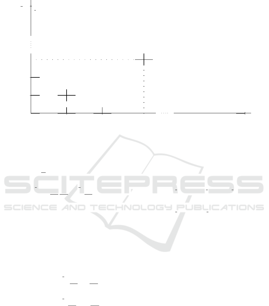
We first demonstrate how the profit function changes
with the total arrival λ where λ
T
= λ
F
(and there-
fore λ
T
= 1/3λ and λ
F
= 2/3λ). In Figure 3 we plot
the profit function for different yard sizes. The price
function is the fixed cost of the lease (c
s
S) plus an in-
come that is increasing and concave with the arrival
rate. Therefore, while bigger yards provide consider-
ably higher profits when the arrival rate is sufficiently
large, they require a higher threshold arrival rate to
provide be profitable in the first place.
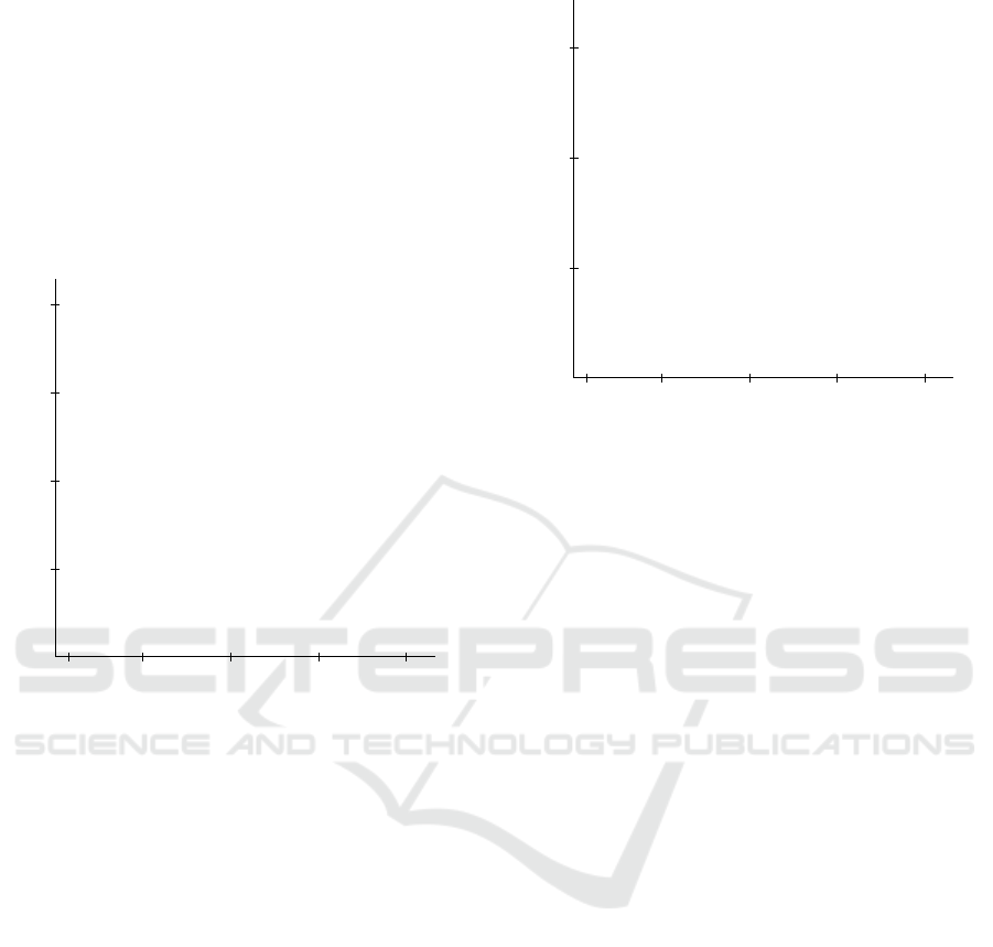
In many cases the yard owner can expand or con-
tract the yard size by leasing space from or to neigh-
boring yards. In Figure 4 we plot the profit as a func-
tion of the yard size for different levels of arrival rates.
The profit function is a sum of an increasing concave
net income and a lease cost that is decreasing linearly
with the lot size. Therefore, for a fixed arrival rate
level, if the yard is very small then (assuming that
the storage price is greater than the unit lease cost)
increasing the lot size is profitable. However, for a
sufficiently large lot, the rejection rate is sufficiently
low that the decrease in container rejection due to an
6
-
200
400
600
50 100 150 2002
S
Yard size
Profit
..........
.
.
.
.
.
.
.
.
.
.
.
.
.
.
.
.
.
.
.
.
.
.
.
.
.
.
.
.
.
.
.
.
.
.
.
.
.
.
.
.
.
.
.
.
.
.
.
.
.
.
.
.
.
.
.
.
.
.
.
.
.
.
.
.
.
.
.
.
.
.
.
.
.
.
.
.
.
.
.
.
.
.
.
.
.
.
.
.
.
.
.
.
.
.
.
.
.
.
.
.
.
.
.
.
.
.
.
.
.
.
.
.
.
.
.
.
.
.
.
.
.
.
.
.
.
.
.
.
.
.
.
.
.
.
.
.
.
.
.
.
.
.
.
.
.
.
.
.
.
.
.
.
.
.
.
.
.
.
.
.
.
.
.
.
.
.
.
.
.
.
.
.
.
.
.
.
.
.
.
.
.
.
.
.
.
.
.
.
.
.
.
.
.
.
.
.
.
.
.
.
.
.
.
.
λ = 45
..........
.
.
.
.
.
.
.
.
.
.
.
.
.
.
.
.
.
.
.
.
.
.
.
.
.
.
.
.
.
.
.
.
.
.
.
.
.
.
.
.
.
.
.
.
.
.
.
.
.
.
.
.
.
.
.
.
.
.
.
.
.
.
.
.
.
.
.
.
.
.
.
.
.
.
.
.
.
.
.
.
.
.
.
.
.
.
.
.
.
.
.
.
.
.
.
.
.
.
.
.
.
.
.
.
.
.
.
.
.
.
.
.
.
.
.
.
.
.
.
.
.
.
.
.
.
.
.
.
.
.
.
.
.
.
.
.
.
.
.
.
.
.
.
.
.
.
.
.
.
.
.
.
.
.
.
.
.
.
.
.
.
.
.
.
.
.
.
.
.
.
.
.
.
.
.
.
.
.
.
.
.
.
.
.
.
.
.
.
.
.
.
.
.
.
.
.
.
.
.
.
.
.
.
.
.
.
.
.
.
.
.
.
.
.
.
.
.
.
.
.
.
.
.
.
.
.
.
.
.
.
.
.
.
.
.
.
.
.
.
.
.
.
.
.
.
.
.
.
.
.
.
.
.
.
.
.
.
.
.
.
.
.
.
.
.
.
.
.
.
.
.
.
.
.
.
.
.
.
.
.
.
.
.
.
.
.
.
.
.
.
.
.
.
.
.
.
.
.
.
.
.
.
.
.
.
.
.
.
.
.
.
.
.
.
.
.
.
.
.
.
.
.
.
.
.
.
.
.
.
.
.
.
.
.
.
.
.
.
.
.
.
.
.
.
.
.
.
.
.
.
.
.
.
.
.
.
.
.
.
.
.
.
.
.
.
.
.
.
.
.
.
.
.
.
.
.
.
.
.
.
.
.
.
.
.
.
.
.
.
.
.
.
.
.
.
.
.
.
.
.
.
.
.
.
.
.
.
.
.
.
.
.
.
.
.
.
.
.
.
.
.
.
.
.
.
.
.
.
.
.
.
.
.
.
.
.
.
.
.
.
.
.
.
.
.
.
.
.
.
.
.
.
.
.
.
.
.
.
.
.
.
.
.
.
.
.
.
.
.
.
.
.
.
.
.
.
.
.
.
.
.
.
.
.
.
.
.
.
.
.
.
.
.
.
.
.
.
.
.
.
.
.
.
.
.
.
.
λ = 90
.
.
.
.
.
.
.
.
.
.
.
.
.
.
.
.
.
.
.
.
.
.
.
.
.
.
.
.
.
.
.
.
.
.
.
.
.
.
.
.
.
.
.
.
.
.
.
.
.
.
.
.
.
.
.
.
.
.
.
.
.
.
.
.
.
.
.
.
.
.
.
.
.
.
.
.
.
.
.
.
.
.
.
.
.
.
.
.
.
.
.
.
.
.
.
.
.
.
.
.
.
.
.
.
.
.
.
.
.
.
.
.
.
.
.
.
.
.
.
.
.
.
.
.
.
.
.
.
.
.
.
.
.
.
.
.
.
.
.
.
.
.
.
.
.
.
.
.
.
.
.
.
.
.
.
.
.
.
.
.
.
.
.
.
.
.
.
.
.
.
.
.
.
.
.
.
.
.
.
.
.
.
.
.
.
.
.
.
.
.
.
.
.
.
.
.
.
.
.
.
.
.
.
.
.
.
.
.
.
.
.
.
.
.
.
.
.
.
.
.
.
.
.
.
.
.
.
.
.
.
.
.
.
.
.
.
.
.
.
.
.
.
.
.
.
.
.
.
.
.
.
.
.
.
.
.
.
.
.
.
.
.
.
.
.
.
.
.
.
.
.
.
.
.
.
.
.
.
.
.
.
.
.
.
.
.
.
.
.
.
.
.
.
.
.
.
.
.
.
.
.
.
.
.
.
.
.
.
.
.
.
.
.
.
.
.
.
.
.
.
.
.
.
.
.
.
.
.
.
.
.
.
.
.
.
.
.
.
.
.
.
.
.
.
.
.
.
.
.
.
.
.
.
.
.
.
.
.
.
.
.
.
.
.
.
.
.
.
.
.
.
.
.
.
.
.
.
.
.
.
.
.
.
.
.
.
.
.
.
.
.
.
.
.
.
.
.
.
.
.
.
.
.
.
.
.
.
.
.
.
.
.
.
.
.
.
.
.
.
.
.
.
.
.
.
.
.
.
.
.
.
.
.
.
.
.
.
.
.
.
.
.
.
.
.
.
.
.
.
.
.
.
.
.
.
.
.
.
.
.
.
.
.
.
.
.
.
.
.
.
.
.
.
.
.
.
.
.
.
.
.
.
.
.
.
.
.
.
.
.
.
.
.
.
.
.
.
.
.
.
.
.
.
.
.
.
.
.
.
.
.
.
.
.
.
.
.
.
.
.
.
.
.
.
.
.
.
.
.
.
.
.
.
.
.
.
.
.
.
.
.
.
.
.
.
.
.
.
.
.
.
.
.
.
.
.
.
.
.
.
.
.
.
.
.
.
.
.
.
.
.
.
.
.
.
.
.
.
.
.
.
.
.
.
.
.
.
.
.
.
.
.
.
.
.
.
.
.
.
.
.
.
.
.
.
.
.
.
.
.
.
.
.
.
.
.
.
.
.
.
.
.
.
.
.
.
.
.
.
.
.
.
.
.
.
.
.
.
.
.
.
.
.
.
.
.
.
.
.
.
.
.
.
.
.
.
.
.
.
.
.
.
.
.
.
.
.
.
.
.
.
.
.
.
.
.
.
.
.
.
.
.
.
.
.
.
.
.
.
.
.
.
.
.
.
.
.
.
.
.
.
.
.
.
.
.
.
.
.
.
.
.
.
.
.
.
.
.
.
.
.
.
.
.
.
.
.
.
.
.
.
.
.
.
.
.
.
.
.
.
.
.
.
.
.
.
.
.
.
.
.
.
.
.
.
.
.
.
.
.
.
.
.
.
.
.
.
.
.
.
.
.
.
.
.
.
.
.
.
.
.
.
.
.
.
.
.
.
.
.
.
.
.
.
.
.
.
.
.
.
.
.
.
.
.
.
.
.
.
.
.
.
.
.
.
.
.
.
.
.
.
.
.
.
.
λ = 135
..........
.
.
.
.
.
.
.
.
.
.
.
.
.
.
.
.
.
.
.
.
.
.
.
.
.
.
.
.
.
.
.
.
.
.
.
.
.
.
.
.
.
.
.
.
.
.
.
.
.
.
.
.
.
.
.
.
.
.
.
.
.
.
.
.
.
.
.
.
.
.
.
.
.
.
.
.
.
.
.
.
.
.
.
.
.
.
.
.
.
.
.
.
.
.
.
.
.
.
.
.
.
.
.
.
.
.
.
.
.
.
.
.
.
.
.
.
.
.
.
.
.
.
.
.
.
.
.
.
.
.
.
.
.
.
.
.
.
.
.
.
.
.
.
.
.
.
.
.
.
.
.
.
.
.
.
.
.
.
.
.
.
.
.
.
.
.
.
.
.
.
.
.
.
.
.
.
.
.
.
.
.
.
.
.
.
.
.
.
.
.
.
.
.
.
.
.
.
.
.
.
.
.
.
.
.
.
.
.
.
.
.
.
.
.
.
.
.
.
.
.
.
.
.
.
.
.
.
.
.
.
.
.
.
.
.
.
.
.
.
.
.
.
.
.
.
.
.
.
.
.
.
.
.
.
.
.
.
.
.
.
.
.
.
.
.
.
.
.
.
.
.
.
.
.
.
.
.
.
.
.
.
.
.
.
.
.
.
.
.
.
.
.
.
.
.
.
.
.
.
.
.
.
.
.
.
.
.
.
.
.
.
.
.
.
.
.
.
.
.
.
.
.
.
.
.
.
.
.
.
.
.
.
.
.
.
.
.
.
.
.
.
.
.
.
.
.
.
.
.
.
.
.
.
.
.
.
.
.
.
.
.
.
.
.
.
.
.
.
.
.
.
.
.
.
.
.
.
.
.
.
.
.
.
.
.
.
.
.
.
.
.
.
.
.
.
.
.
.
.
.
.
.
.
.
.
.
.
.
.
.
.
.
.
.
.
.
.
.
.
.
.
.
.
.
.
.
.
.
.
.
.
.
.
.
.
.
.
.
.
.
.
.
.
.
.
.
.
.
.
.
.
.
.
.
.
.
.
.
.
.
.
.
.
.
.
.
.
.
.
.
.
.
.
.
.
.
.
.
.
.
.
.
.
.
.
.
.
.
.
.
.
.
.
.
.
.
.
.
.
.
.
.
.
.
.
.
.
.
.
.
.
.
.
.
.
.
.
.
.
.
.
.
.
.
.
.
.
.
.
.
.
.
.
.
.
.
.
.
.
.
.
.
.
.
.
.
.
.
.
.
.
.
.
.
.
.
.
.
.
.
.
.
.
.
.
.
.
.
.
.
.
.
.
.
.
.
.
.
.
.
.
.
.
.
.
.
.
.
.
.
.
.
.
.
.
.
.
.
.
.
.
.
.
.
.
.
.
.
.
.
.
.
.
.
.
.
.
.
.
.
.
.
.
.
.
.
.
.
.
.
.
.
.
.
.
.
.
.
.
.
.
.
.
.
.
.
.
.
.
.
.
.
.
.
.
.
.
.
.
.
.
.
.
.
.
.
.
.
.
.
.
.
.
.
.
.
.
.
λ = 180
Figure 4: The profit as a function of the yard size for differ-
ent total arrival levels.
additional spot does not offset its lease cost and there-
fore profits will decrease if the yard size is increased.
In our example, when λ = 45 then the optimal lot size
is very small, S
∗
= 35, whereas in a lot with λ = 180
then the optimal size is S
∗
= 161. In this analysis of
the optimal yard size we do not take into account pos-
sible future growth in the customers’ arrivals rate. See
Giat (2018) for an analysis of such a situation.
5 CONCLUSION
This paper was motivated by a small storage yard
that temporarily stores containers for a short period
of time before they are transported to a neighboring
marine port. The vast majority of containers that are
stored in the yard are either the 20 feet TEU or its ex-
actly double counterpart, the forty feet TEU. We de-
scribe the two storage services that the yard provides
and show that if the proportional fee is equal to the
one-time fee multiplied by the expected duration then
the two schemes provide the same profits.
The numerical illustration shows the profit func-
tion’s properties. When viewed as function of the yard
size, it is a sum of a linearly increasing cost and an
increasing concave revenue and therefore there is an
optimal yard size. For the yard to be profitable, there
is a minimal necessary arrival rate. This threshold is
increasing with the yard size and therefore large yards
are initially at a disadvantage. However, if yard own-
ers are confident that there will be sufficiently many
customers, then they the larger yards will secure them
greater profits.
Storage Fees in a Container Yard with Multiple Customer Types
183

While the numerical analysis in this paper is lim-
ited to a two-type customer model, this paper also lays
the foundation to analyzing more complex settings
with multiple client types. Such an analysis can focus
on questions about whether it is beneficial to preemp-
tively reject smaller clients in order to secure space
for larger (and perhaps more profitable) customers.
REFERENCES
Chan, H., Xu, S., and Qi, X. (2019). A comparison of time
series methods for forecasting container throughput.
International Journal of Logistics Research and Ap-
plications, 22(3):294–303.
Dong, J. and Song, D. (2012). Lease term optimisation in
container shipping systems. International Journal of
Logistics Research and Applications, 15(2):87–107.
Dreyfuss, M. and Giat, Y. (2017). Optimizing spare battery
allocation in an electric vehicle battery swapping sys-
tem. In Proceedings of the 6th International Confer-
ence on Operations Research and Enterprise Systems,
pages 38–46. SCITEPRESS.
Federgruen, A. and Green, L. (1984). An m/g/c queue in
which the number of servers required is random. Jour-
nal of Applied Probability, 21(3):583–601.
Fletcher, G., Perros, H., and Stewart, W. (1986). A queue-
ing system where customers require a random number
of servers simultaneously. European Journal of Oper-
ational Research, 23:331–342.
Giat, Y. (2018). Principal-agent analysis on how legal risks
affect audit fees and quality. International Journal of
Strategic Decision Sciences, 9(3):113–126.
Green, L. (1980). A queueing system in which customers
require a random number of servers. Operations Re-
search, 28(6):1335–1346.
Green, L. (1981). Comparing operating characteristics of
queues in which customers require a random number
of servers. Management Science, 27(1):65–74.
Hassin, R., Shaki, Y., and Yovel, U. (2015). Optimal
service-capacity allocation in a loss system. Naval Re-
search Logistics, 62(2):81–97.
ISO (2020). Iso 668:2020 series 1 freight containers —
classification, dimensions and ratings. Available at
https://www.iso.org/standard/76912.html.
Kaufman, J. (1981). Blocking in a shared resource en-
vironment. IEEE Transactions on communications,
29(10):1474–1481.
Marchet, G., Melacini, M., Perotti, S., and Tappia, E.
(2012). Analytical model to estimate performances
of autonomous vehicle storage and retrieval systems
for product totes. International Journal of Production
Research, 50(24):7134–7148.
Moscholios, I., Vassilakis, V., Logothetis, M., and Boucou-
valas, A. (2016). A probabilistic threshold-based
bandwidth sharing policy for wireless multirate loss
networks. IEEE Wireless Communications Letters,
5(3):304–307.
Notteboom, T., Pallis, A., and Rodrigue, J. (2020). Port
Economics, Management and Policy. Routledge, New
York.
Woo, Y., Song, J., and Kim, K. (2016). Pricing storage of
outbound containers in container terminals. Flexible
Services and Manufacturing Journal, 28(4):644–668.
Yu, M., Kim, K., and Lee, C. Y. (2011). Inbound container
storage pricing schemes. IIE Transactions, 47(8):800–
818.
Zhang, B., Ng, C., and Cheng, T. C. (2014). Multi-period
empty container repositioning with stochastic demand
and lost sales. Journal of the Operational Research
Society, 65(2):302–319.
ICORES 2021 - 10th International Conference on Operations Research and Enterprise Systems
184
