Post-hoc Explanation using a Mimic Rule for Numerical Data
Kohei Asano and Jinhee Chun
Graduate School of Information Sciences, Tohoku University, Sendai, Japan
Keywords:
Explanations, Transparency, Rules.
Abstract:
We propose a novel rule-based explanation method for an arbitrary pre-trained machine learning model. Gen-
erally, machine learning models make black-box decisions that are not easy to explain the logical reasons to
derive them. Therefore, it is important to develop a tool that gives reasons for the model’s decision. Some
studies have tackled the solution of this problem by approximating an explained model with an interpretable
model. Although these methods provide logical reasons for a model’s decision, a wrong explanation some-
times occurs. To resolve the issue, we define a rule model for the explanation, called a mimic rule, which
behaves similarly in the model in its region. We obtain a mimic rule that can explain the large area of the
numerical input space by maximizing the region. Through experimentation, we compare our method to earlier
methods. Then we show that our method often improves local fidelity.
1 INTRODUCTION
Recently, machine learning models produce highly
accurate predictions that are applied to various tasks.
Because these models tend to be complex and lacking
transparency, humans might have difficulty interpret-
ing their decisions. Interpretability and transparency
issues present urgent difficulties to be resolved in the
machine learning field. Especially, it presents se-
vere difficulty when applied to sensitive fields such
as credit risks(Rudin and Shaposhnik, 2019), educa-
tions(Lakkaraju et al., 2015), and health care(Caruana
et al., 2015).
Many studies have been conducted recently to im-
prove machine learning model transparency(Guidotti
et al., 2018b). Among the approaches are meth-
ods that build another explanatory model approxi-
mating a pre-trained model ex-post. Such meth-
ods are called post-hoc explanations. Such meth-
ods are preferably model-agnostic, meaning that they
are applicable to any machine learning model with-
out knowing model details. Because of these prop-
erties, post-hoc explanation can be widely applicable
to tabular data(Guidotti et al., 2018a), image(Ribeiro
et al., 2016; Ribeiro et al., 2018), and sentiment pre-
diction(Ribeiro et al., 2016).
Although post-hoc explanations are a useful and
applicable framework, several issues must be re-
solved for further improvement. First, to exploit
the internal decision rule of a black-box model,
this method approximates a black-box model using
other interpretable machine learning such as a linear
model(Ribeiro et al., 2016; Lundberg and Lee, 2017)
or a decision tree(Guidotti et al., 2018a). The approx-
imation model sometimes has insufficient accuracy;
it can lead to an incorrect explanation(Rudin, 2019).
Moreover, although the explanatory model approxi-
mates a black-box model locally, the applicable scope
is unclear. Therefore, the explanatory model cannot
be used globally. It is therefore necessary to develop
a more accurate and globally applicable post-hoc ex-
planation method.To resolve these issues, we propose
a novel rule-based explanation method: Mimic Rule
Explanation (MRE). The MRE explanation consists
of a rule that mimics the black-box model we call
a mimic rule. Users can readily derive the decision
using only a mimic rule because a mimic rule is an
interpretable rule model representing the region with
the same decision. Because of the mimic rule prop-
erty, the MRE explanation shows higher correctness
than the previous rule-based explanation method. The
contributions of our study are the following.
1. We formulate a novel rule-based explanation
method using a mimic rule and propose an algo-
rithm to construct the explanation.
2. We show parameter-dependence and comparison
of earlier methods with illustrative results.
3. Our method generates a more accurate explana-
tory rule than the earlier rule-based explanation
method.
768
Asano, K. and Chun, J.
Post-hoc Explanation using a Mimic Rule for Numerical Data.
DOI: 10.5220/0010238907680774
In Proceedings of the 13th International Conference on Agents and Artificial Intelligence (ICAART 2021) - Volume 2, pages 768-774
ISBN: 978-989-758-484-8
Copyright
c
 2021 by SCITEPRESS – Science and Technology Publications, Lda. All rights reserved

2 RELATED WORK
One approach to enhancing interpretability is build-
ing globally interpretable and highly accurate ma-
chine learning models such as those of rule lists
(Wang and Rudin, 2015; Angelino et al., 2017), and
rule sets (Lakkaraju et al., 2016; Wang, 2018; Dash
et al., 2018). Users can clearly comprehend model
behaviors and explanations of any decision. Espe-
cially, rule models give users simple logic based on
If-Then statements. They are often applied in inter-
pretable/explainable machine learning. These models
become simple to interpret. Therefore, they present
difficulty when performing highly accurate analyses
of problems with a complex input domain.
Lakkaraju et al. (Lakkaraju et al., 2016) demon-
strated through a user study that disjoint rule sets pro-
vide high interpretability to users. As a method of
explaining any machine learning model, Ribeiro et al.
(Ribeiro et al., 2016; Lundberg and Lee, 2017) pro-
posed a locally interpretable model-agnostic explana-
tion framework. It uses an explanatory model to ex-
hibit the behavior of black-box models to users. In
fact, it locally approximates a black-box model us-
ing a sparse linear model. Then users can understand
the model behavior using explanatory model weights.
Ribeiro et al. (Ribeiro et al., 2018) also proposed an-
other local model-agnostic explanation system called
Anchor , which uses an important feature set as an
explanatory model.
Some studies(Laugel et al., 2019; Aivodji et al.,
2019; Rudin, 2019) have specifically examined the
danger of post-hoc explanations. Post-hoc explain-
ers(Ribeiro et al., 2016; Ribeiro et al., 2018; Guidotti
et al., 2018a) sometimes provide an incorrect expla-
nation. That is, they cannot capture the behavior of
the black-box model because of approximation. Our
explanatory method does not approximate the black-
box model with another interpretable machine learn-
ing model. It improves the descriptions of the model
by constructing the explanatory rule with geometric
consideration. Moreover, we surmise that the post-
hoc explanation still has an important aspect because
users cannot necessarily use the information of a ma-
chine learning model like the training data of the pre-
trained machine learning data in practical terms.
3 PRELIMINARIES
We show the notations and definitions and show
previous rule-based explanation methods: Anchor
(Ribeiro et al., 2018) and LORE (Guidotti et al.,
2018a).
3.1 Notations and Definition
We denote the indicator function by I(c) where I(c)
returns 1 if a condition c is satisfies, and otherwise 0.
We also denote a set of features by [d] =
{
1, . . . , d
}
.
For a set A, |A| is a cardinality of A.
We denote notations of a classification problem
using a tabular dataset. A black box classifier is
f : R
d
→ C , where, the domain of f is d-dimensional
numeric features and C is a target space and set of
classes. Consequently, for any instance x, y = f (x) is
the label assigned by the model f to x.
Because we consider post-hoc explanations, we
do not assume f and internal information of f . For
example, if the model is a neural network, then infor-
mation such as network construction or weighting is
not used.
A rule-based explanation E is formulated as a tu-
ple of a rule R and a label y:
E = (R, y). (1)
This definition is similar to an association rule. There-
fore, if it satisfies x ∈ R, it is expected that f (x) = y.
A rule is a subspace of input space R ⊂ R
d
and is
represented as a Cartesian product of each feature’s
interval.
R =
d
∏
i=1
R
i
=
d
∏
i=1
[a
i
, b
i
]. (2)
It is a readable model. Users can understand the be-
havior of the black-box model using the rule.
3.2 Previous Methods
3.2.1 Anchor
The explanations of Anchor consist of a set of dis-
cretized features. In the anchor algorithm, the in-
put space is converted to discretized space called
an interpretable representation(Ribeiro et al., 2018;
Lundberg and Lee, 2017). It is expected to assign
the corresponding label by the black-box model with
high probability if instances that contain the feature
set.Anchor generates the interpretable feature set with
the beam-search and KL-LUCB algorithm(Kaufmann
and Kalyanakrishnan, 2013) for a multi-armed bandit
problem.
When Anchor applies data having a continuous
feature, the feature is converted to categorical fea-
tures by splitting. This process lacks ordering of a
continuous feature. Because the feature set is formu-
lated in the interpretable feature space and because
this space has a gap separating the input space, the
Post-hoc Explanation using a Mimic Rule for Numerical Data
769

explanation might not be accurate in the input space.
Anchor sometimes fails to show an explanation when
applied to an imbalanced labeled dataset.
3.2.2 LORE
LORE uses a decision tree model(Guidotti et al.,
2018a) as the explanatory rule. The decision tree lo-
cally approximates the black-box model near an ex-
plained instance x. The decision tree is trained with
the data that is generated by a genetic algorithm(Tsai
et al., 2013). Using an appropriate evaluation function
for a genetic algorithm, it can generate data that have
good properties: neighborhood of x and balanced la-
bels.
The LORE’s explanation is local approxima-
tion with a decision tree, thereby the possibility
exists that the rule includes the incorrect region:
{
z ∈ R : f (z) 6= f (x)
}
. A rule of a decision tree would
consist of infinite intervals: (a
i
= −∞ or b
i
= +∞ in
eq. (2)). Moreover, it causes low accuracy of the ex-
planatory rule. Genetic algorithms often cannot gen-
erate appropriate training data. For example, if an
explained instance is far from the decision boundary,
then a genetic algorithm might be able to generate bal-
anced labeled data.
4 PROPOSED METHOD
We propose a novel explanation method, Mimic rule
explanation (MRE), that approximates a black box
model more strictly than previous rule-based expla-
nation methods. First, we define the explanatory rule,
which we designate as a mimic rule. To solve a mimic
rule, we introduce an approximated formulation. The
algorithm for mimic rules is summarized at the end of
the section.
4.1 Definition of a Mimic Rule
We define a mimic rule as a cartesian product of each
features’ finite intervals. A mimic rule also follows
eq. (2) and is denoted by R
M
.
R
M
=
d
∏
i=1
R
M,i
=
d
∏
i=1
[a
i
, b
i
] (a
i
, b
i
∈ R). (3)
By defining with a cartesian product of finite inter-
vals, it prevents an explanatory rule including an in-
correct region. Moreover, we require that a mimic
rule satisfy the following two properties.
• Correctness: For any instance x in a mimic rule
R
M
, it is assigned a label y by f . Consequently,
the following is satisfied:
∀z ∈ R
M
, f (z) = y. (4)
The mimic rule behaves similarly to model f if
this is satisfied. Consequently, the mimic rule
does not include an incorrect region. It is useful
as an alternative to the model.
• Maximality: A mimic rule is a maximal rule. If
a mimic rule is expanded, then the property (4) is
not satisfied. By presenting a maximal rule, the
explanation covers a large part of the input space.
It is therefore more preferred as an explanation.
Innumerable mimic rules can satisfy correctness and
maximality properties because the input space is con-
tinuous. Nevertheless, we presume that MRE presents
a mimic rule as an explanatory rule in this study.
Fig. 1a shows an intuitive illustration of a mimic rule
in the input space.
Since it is difficult to find a mimic rule in the con-
tinuous input space, we discretize the input space and
consider a mimic rule in the discretized space.
Fig. 1b portrays a mimic rule in the discretized
input space. It is noteworthy that multiple mimic
rules can exist in the discretized space. However, the
number of rules is countable. Although discretiza-
tion of a continuous feature is used in many related
works(Ribeiro et al., 2018; Angelino et al., 2017;
Rudin and Shaposhnik, 2019), these studies handle a
discretized feature as a categorical feature and deprive
the ordering of the feature. By handling discretized
points as prototypes of the feature, ordering of a fea-
ture is maintained. We denote the prototypes of i-th
feature (i ∈ [d]) as S
i
S
i
=

x
i,−m
−
, . . . , x
i,−1
, x
i,0
, x
i
1
, . . . , x
i,m
+

. (5)
where x
i,0
= x
i
, and m
−
, m
+
are a natural number that
controls a number of quantiles. For the sake of sim-
plicity, we assume m = m
−
= m
+
and x
i, j
− x
i, j−1
=
ε (−m < j ≤ m) with a constant ε. Hence the dis-
cretized space S can be define with S
i
as bellow:
S =
d
∏
i=1
S
i
. (6)
(a) The input space (b) The discretized space
Figure 1: Illustration of a mimic rule in the input space (a)
and the discretized space (b).
ICAART 2021 - 13th International Conference on Agents and Artificial Intelligence
770

4.2 Algorithm for a Mimic Rule
We propose an algorithm that presents a mimic rule
in discretized input space. It satisfies correctness and
maximality properties. Note that a mimic rule in the
discretized input might not satisfy the properties in
the original input space. We summarize the algorithm
as 1.
First, we simplify the problem with parameters to
solve a mimic rule in practical computational time.
The algorithm constructs a mimic rule by expanding
a region of the rule from the explained instance. In-
stances in space S might be evaluated by model f in
the algorithm. Here, if all instances in the space S are
evaluated by f , we can get an ideal mimic rule in S.
However, large amounts of computation time must
be used because of the number of instances: |S| ex-
ist in combinatorial order. For example, even in case
of ∀i ∈ [d], |S
i
| = 2, the number of instances in S
is 2
d
. To avoid this issue, we introduce parameter
P ∈ N, 1 ≤ P ≤ d that controls the search space size.
We consider instances that are combinatorially per-
turbed up to P. The neighbor instances X
q
(S), which
are perturbed features in a set q ∈ 2
[d]
, are denoted as
presented below.
X
q
(S) =
d
∏
i=1
X
q,i
(S), (7)
X
q,i
(S) =
(
S
i
\
{
x
i
}
(i ∈ q)
{
x
i
}
otherwise
. (8)
Therefore, the set of instances which might be evalu-
ated is
[
q∈2
[d]
:|q|≤P
X
q
(S). (9)
When the cardinality of q is large, |X
q
(S)| exists in
exponential order with respect to the number of pro-
totypes. Thereby, the cardinality eq. (9) would be
huge. To constrain the number of evaluated instances,
we introduce a parameter N ∈ N and evaluate N in-
stances sampled from X
q
(S).
This algorithm repeats evaluation of neighbor in-
stances and shrinking the search space. For evalua-
tion, N neighbor instances are sampled from X
q
(S);
Z denotes the set of sampled instances. Here the i-th
features (i ∈ q) of the instances is perturbed. Next,
we evaluate the instances z ∈ Z with given model f .
The set of instances assigned the different label from
f (x) is denoted as Z
−
. Because a mimic rule does
not include negative instances inside itself, the search
space is shrunk to exclude the instances in Z
−
with a
function ShrinkSearchSpace in Algorithm 1. Such
evaluation is repeated until p reaches P. It returns the
mimic rule as:
R
M
=
d
∏
i=1
[min
{
S
i
}
, max
{
S
i
}
] (10)
at the end of the algorithm.
In the shrinking part of the algorithm, we use set
V ⊆ S, which is a region that has no negative instances
inside of itself. At the initial step of this process, V
only consists of the explained instance x. The shrink-
ing process continues until there are no instances to
expand the sum of |S
i
\V
i
| for i ∈ q of zero. Region
V
i
is expanded with a prototype x
i, j
that is the near-
est from the edge of V
i
. The region is updated if the
expanded region does not include negative instances.
Otherwise, the prototypes that are outside of x
i, j
are
removed from S
i
.
In the implementation, every S
i
is represented with
a list structure. Every element is sorted in ascending
order based on the absolute value of the index. We
consider a Pop(L) method that returns the left edge
element of the list L.
Algorithm 1: Construction algorithm for a mimic rule.
Require: Classifier f , explained instance x, search
space S, parameters P, N
Ensure: Mimic rule R
M
for all p ∈
{
1, . . . , P
}
do
for all q ∈
n
Q ∈ 2
[d]
: |Q| = p
o
do
Z ← sample N instances from X
q
(S)
Z
−
←
{
z ∈ Z : f (z) 6= f (x)
}
S ← ShrinkSearchSpace(S, Z
−
, q)
end for
end for
for all i ∈
{
1, . . . , d
}
do
R
M,i
← [min
{
S
i
}
, max
{
S
i
}
]
end for
return R
M
function SHRINKSEARCHSPACE(S, Z
−
, q)
V ←
∏
d
i=1
[x
i
, x
i
]
while
∑
i∈q
|S
i
\V
i
| > 0 do
i ← pick from q that satisfies |S
i
\V
i
| > 0
x
i, j
← Pop(S
i
\V
i
)
R
0
← expand V
i
with x
i, j
if ∀z ∈ Z
−
, z ∈ V
0
then
remove outside elements of x
i, j
from S
i
else
V ← V
0
end if
end while
return S
end function
Post-hoc Explanation using a Mimic Rule for Numerical Data
771

5 EXPERIMENTS
We next evaluate our explanation method. We present
two experiments: qualitative evaluation with an illus-
trative example and quantitative evaluation of expla-
nations’ fidelity.
We implemented MRE (Algorithm 1), LORE and
scripts for all experiments in Python 3.7. For im-
plementation, we use an open source machine learn-
ing library scikit-learn
1
, Ribeiro’s anchor implemen-
tation
2
. All experiments are run with a Linux ma-
chine with 3.40 GHz Intel Core-i7 CPU and 8.0GB of
RAM.
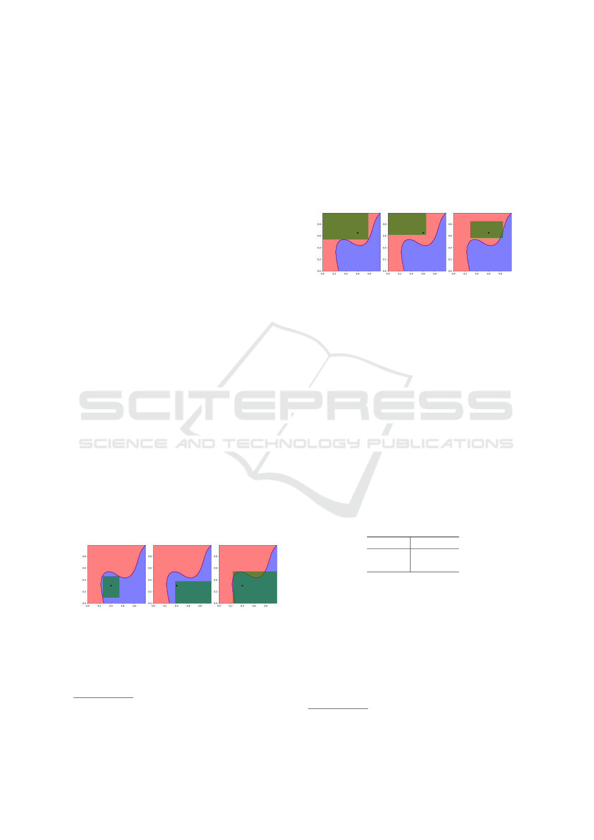
5.1 Illustrative Examples
To present insights about characteristics of our
method and dependency of parameters, we used a
two-dimensional half-moon dataset. As a classifier,
we use the SVC that trains with default hyperparam-
eters of scikit-learn library. Fig. 2 shows the mimic
rules under each conditions. The left image of Fig. 2
presents a mimic rule applied under numerous quan-
tiles (m = 25) and all samples in search space S. Ac-
tually, MRE can present an almost ideal mimic rule
in such a condition. Given a low number of quan-
tiles (m = 4) in the center image of Fig. 2, a mimic
rule might not satisfy the maximality. This issue
arises because the distance between search points is
large and because the adjacent search point crosses
the decision boundary of the model. The condi-
tion under which a low number of samples N might
lose the correctness property (right image of Fig. 2)
occurs because the negative samples in the search
space

z ∈ X
q
(S) : f (z) 6= y

are not sampled. Con-
sequently, the rule expands improperly because of the
low number of samples.
Figure 2: Illustrative result of a mimic rule (green area) with
a half-moon dataset. Left: m = 25, N = |X
q
(S)|, Center:
m = 5, N = |X
q
(S)|, Right: m = 25, N = 10.
We show the difference between Anchor, LORE, and
our method in Fig. 3. Our method uses computation
with numerous quantiles (m = 25) and a large number
1
https://scikit-learn.org/
2
https://github.com/marcotcr/anchor
of samples. In this condition, our method can gener-
ate a maximal and correct mimic rule (left image of
Fig. 3). The center image of Fig. 3 shows the rule of
Anchor. Although Anchor’s explanatory rule is cor-
rect, i.e. rule does not include incorrect region, the
rule is not maximal. Moreover, LORE’s explanatory
rule is not correct: it includes an incorrect region (blue
area), meaning that LORE presents a wrong explana-
tion for instances in incorrect regions.
Figure 3: Comparison with the explanatory rules (green
area). Left: MRE, Center: Anchor, Right: LORE
5.2 Evaluation of Fidelity
We measure the reliability of the explanatory rule
with the iris dataset and breast-cancer (BC) dataset,
which are opened in the UCI machine learning repos-
itory
3
. Table 1 presents details of the datasets. We
used 80% of datasets as training data and the rest of
20% as test data. As black-box models, we trained
a SVC and multilayer perceptron with default hyper-
parameters of the scikit-learn library. We set the
parameters of Anchor and LORE as the same orig-
inal parameters in their paper(Ribeiro et al., 2018;
Guidotti et al., 2018a). Regarding the parameters of
MRE, we discretized the [0, 1] scaled input space
with m = 11 and ε = 0.05. Then we set N = 10 and
P = 4 for MRE parameters.
Table 1: Details of datasets: #, d denote the number of
whole instances, the number of dimension, respectively.
datasets # d
Iris 150 4
BC 569 30
We use metrics for reliability: correctness and cov-
erage, and eq. (11) and eq. (12) present their defini-
tions. The correctness is measured using the proba-
bility of f (x) = f (z), where z are sampled uniformly
from the explanatory rule, and the instances z for cov-
erage are sampled uniformly from the whole input
domain. Each metric shows the value between 0 to
1 and a higher score means better. High correctness
means that the explanatory rule does not include an
incorrect region as
{
z ∈ R : f (z) 6= f (x)
}
, where high
3
https://archive.ics.uci.edu/ml/index.php
ICAART 2021 - 13th International Conference on Agents and Artificial Intelligence
772

coverage means that the explanatory rule covers large
space over the input domain. Both of these metrics
are measured using 1 million samples.
correctness = E
z∼U(R)
[I ( f (x) = f (z))] (11)
coverage = E
z∼U(X )
[I ( f (x) = f (z))] (12)
Comparison with correctness is presented in Table 2.
MRE shows higher correctness than Anchor and
LORE in every conditions. This fact indicates that
a mimic rule satisfies the required condition: correct-
ness. Actually, LORE works better than Anchor for
the Iris dataset. Although approximation with a de-
cision tree has good accuracy for low-dimensional
data, it does not work well with high-dimensional
data.Some possible causes include the number of
training data for a decision tree. The correctness of
Anchor is lower in all conditions. Anchor presents
the feature set that captures the model well. However,
it is precise in the binarized input space, not in the
original space(Ribeiro et al., 2018). Consequently, bi-
narization and lack of numeric ordering might cause
a low-quality explanation. MRE performs high cor-
rectness by keeping the numeric ordering and by not
approximating using another model. In the result with
BC dataset and SVC, MRE shows lower correctness
than that of other conditions. The decision boundary
of SVC sometimes contains a small region that does
not include training data(Laugel et al., 2019). It leads
to incorrect explanations. Because of the discretiza-
tion of the input space, it might miss such regions and
tend to show low correctness. Consequently, explana-
tions of MRE are more reliable because the explana-
tory rule has high correctness.
Table 2: Comparison of MRE, Anchor and, LORE with the
correctness.
MRE Anchor LORE
Iris SVC 1.000 0.440 0.761
MLP 1.000 0.440 0.656
BC SVC 0.741 0.360 0.351
MLP 0.991 0.388 0.377
Comparison with the coverage is presented in Table 3.
The coverage of MRE tends to be lower than that
of the earlier method.Anchor and LORE show higher
coverage, meaning that their explanatory rule covers
a large area of the input space. The rule of Anchor
and LORE consists of a few conditions of features
and it improves its coverage. However, a mimic rule
consists of many conditions. It causes low coverage.
We consider that there is a trade-off between correct-
ness and coverage. The high-coverage rule might be
easy to interpret for users. However, it gives users a
misunderstanding of the black-box model. The high-
correctness rule covers a small region. Therefore, the
user cannot apply the rule widely, but the rule behaves
similarly to the model: users can use the rule as a sur-
rogate model.
Table 3: Comparison of MRE, Anchor and, LORE with the
coverage.
MRE Anchor LORE
Iris SVC 0.021 0.828 0.182
MLP 0.026 0.813 0.125
BC SVC 0.220 0.603 0.801
MLP 0.085 0.445 0.446
Table 4 presents the correctness with time expended.
MRE finds the explanatory rule faster than other
methods in a low-dimensional dataset. The compu-
tation time of Algorithm 1 increases exponentially
with the number of dimensions. Therefore, it takes
much time in the BC dataset. However, by introduc-
ing the discretization and by constraining the search
space with parameter P, it can compute in practical
time. Anchor presents the explanatory feature set with
beam search(Ribeiro et al., 2018). For that reason, the
computation time increases with the number of bina-
rized dimensions. The computation time of LORE is
almost constant because LORE trains a decision tree
using a constant number of training data. It is note-
worthy that we generate 5000 samples in this experi-
ment.
Table 4: Comparison of MRE, Anchor and, LORE with the
computation time in second.
MRE Anchor LORE
Iris SVC 0.005 0.107 0.250
MLP 0.007 0.250 0.252
BC SVC 16.42 3.457 0.374
MLP 17.45 5.294 0.811
6 CONCLUSIONS
We proposed MRE: a novel local explanation method
using a mimic rule. We defined the mimic rule
as showing an internal decision rule of a black-box
model. To compute a mimic rule effectively, we intro-
duce some approximations and propose the algorithm.
In the experiment with tabular datasets, our method
showed higher fidelity than the previous rule-based
explanation: Anchor and Lore. We showed a tradeoff
between fidelity and coverage experimentally. More-
over, MRE is solved in practical computation time. It
indicates that our method is widely applicable.
Post-hoc Explanation using a Mimic Rule for Numerical Data
773

Our method supports only numerical input.
Therefore to improve the range of application, it must
be extended to the mixed data input: numerical and
categorical data. Although our method shows high fi-
delity in the experiment, coverage is still lower than
those of earlier methods so that improving coverage
is an important task.It remains a global explanation of
a black-box model.
ACKNOWLEDGEMENTS
This work was partially supported by JSPS Kakenhi
20H04143 and 17K00002.
REFERENCES
Aivodji, U., Arai, H., Fortineau, O., Gambs, S., Hara, S.,
and Tapp, A. (2019). Fairwashing: the risk of ra-
tionalization. volume 97 of Proceedings of Machine
Learning Research, pages 161–170, Long Beach, Cal-
ifornia, USA. PMLR.
Angelino, E., Larus-Stone, N., Alabi, D., Seltzer, M., and
Rudin, C. (2017). Learning certifiably optimal rule
lists. In Proceedings of the 23rd ACM SIGKDD In-
ternational Conference on Knowledge Discovery and
Data Mining, pages 35–44. ACM.
Caruana, R., Lou, Y., Gehrke, J., Koch, P., Sturm, M., and
Elhadad, N. (2015). Intelligible models for healthcare:
Predicting pneumonia risk and hospital 30-day read-
mission. In Proceedings of the 21th ACM SIGKDD In-
ternational Conference on Knowledge Discovery and
Data Mining, pages 1721–1730. ACM.
Dash, S., Gunluk, O., and Wei, D. (2018). Boolean decision
rules via column generation. In Advances in Neural
Information Processing Systems, pages 4655–4665.
Guidotti, R., Monreale, A., Ruggieri, S., Pedreschi, D.,
Turini, F., and Giannotti, F. (2018a). Local rule-based
explanations of black box decision systems. arXiv
preprint arXiv:1805.10820.
Guidotti, R., Monreale, A., Ruggieri, S., Turini, F., Gian-
notti, F., and Pedreschi, D. (2018b). A survey of meth-
ods for explaining black box models. ACM Computing
Surveys (CSUR), 51(5):93.
Kaufmann, E. and Kalyanakrishnan, S. (2013). Information
complexity in bandit subset selection. In Conference
on Learning Theory, pages 228–251.
Lakkaraju, H., Aguiar, E., Shan, C., Miller, D., Bhanpuri,
N., Ghani, R., and Addison, K. L. (2015). A ma-
chine learning framework to identify students at risk
of adverse academic outcomes. In Proceedings of
the 21th ACM SIGKDD international conference on
knowledge discovery and data mining, pages 1909–
1918. ACM.
Lakkaraju, H., Bach, S. H., and Leskovec, J. (2016). Inter-
pretable decision sets: A joint framework for descrip-
tion and prediction. In Proceedings of the 22nd ACM
SIGKDD international conference on knowledge dis-
covery and data mining, pages 1675–1684. ACM.
Laugel, T., Lesot, M.-J., Marsala, C., Renard, X., and De-
tyniecki, M. (2019). The dangers of post-hoc inter-
pretability: Unjustified counterfactual explanations.
In Proceedings of the Twenty-Eighth International
Joint Conference on Artificial Intelligence, IJCAI-19,
pages 2801–2807. International Joint Conferences on
Artificial Intelligence Organization.
Lundberg, S. M. and Lee, S.-I. (2017). A unified approach
to interpreting model predictions. In Advances in neu-
ral information processing systems, pages 4765–4774.
Ribeiro, M. T., Singh, S., and Guestrin, C. (2016). Why
should i trust you?: Explaining the predictions of any
classifier. In Proceedings of the 22nd ACM SIGKDD
international conference on knowledge discovery and
data mining, pages 1135–1144. ACM.
Ribeiro, M. T., Singh, S., and Guestrin, C. (2018). An-
chors: High-precision model-agnostic explanations.
In AAAI, pages 1527–1535.
Rudin, C. (2019). Stop explaining black box machine learn-
ing models for high stakes decisions and use inter-
pretable models instead. Nature Machine Intelligence,
1(5):206–215.
Rudin, C. and Shaposhnik, Y. (2019). Globally-consistent
rule-based summary-explanations for machine learn-
ing models: Application to credit-risk evaluation.
SSRN Electronic Journal.
Tsai, C.-F., Eberle, W., and Chu, C.-Y. (2013). Ge-
netic algorithms in feature and instance selection.
Knowledge-Based Systems, 39:240–247.
Wang, F. and Rudin, C. (2015). Falling rule lists. In Artifi-
cial Intelligence and Statistics, pages 1013–1022.
Wang, T. (2018). Multi-value rule sets for interpretable
classification with feature-efficient representations. In
Bengio, S., Wallach, H., Larochelle, H., Grauman, K.,
Cesa-Bianchi, N., and Garnett, R., editors, Advances
in Neural Information Processing Systems 31, pages
10835–10845. Curran Associates, Inc.
ICAART 2021 - 13th International Conference on Agents and Artificial Intelligence
774