
Drivable Area Extraction based on Shadow Corrected Images
Mohamed Sabry
1 a
, Mostafa El Hayani
1 b
, Amr Farag
2 c
, Slim Abdennadher
1 d
and Amr El Mougy
1 e
1
Computer Science Department, German University in Cairo, Cairo, Egypt
2
Mechatronics Department, German University in Cairo, Cairo, Egypt
Keywords:
Shadow Removal, Monocular Camera, Computer Vision, Image Processing, Unstructured Roads.
Abstract:
Drivable area detection is a complex task that needs to operate efficiently in any environmental condition to
ensure wide adoption of autonomous vehicles. In the case of low cost camera-based drivable area detection,
the spatial information is required to be uniform as much as possible to ensure the robustness and reliability
of the results of any algorithm in most weather and illumination conditions. The general change in illumina-
tion and shadow intensities present a significant challenge and can cause major accidents if not considered.
Moreover, drivable area detection in unstructured environments is more complex due to the absence of vital
spatial information such as road markings and lanes. In this paper, a shadow reduction approach combining
Computer Vision (CV) - Image Processing (IM) with Deep Learning (DL) is used on a low cost monocular
camera based system for reliable and uniform shadow removal. In addition, a validation test is applied with a
DL model to validate the approach. This system is developed for the Self-driving Car (SDC) lab at the German
University in Cairo (GUC) and is to be used in the shell eco-marathon autonomous competition 2021.
1 INTRODUCTION
Drivable area detection is a crucial module that is ex-
pected to be faultless in segmenting the road to en-
sure the safety of any autonomous vehicle as well as
other traffic participants. This requires the received
data from the vehicle perception to be highly reliable
in most conditions including varying weather condi-
tions and unstructured roads.
Autonomous vehicles typically utilize one of three
sensor setups in the perception module to extract the
drivable area: a full sensor setup which fuses the
data from LiDARs, RADARs and cameras and op-
erates under no power or processing restrictions, the
Lidar only setup which is also under the high pro-
cessing power category, and the final setting which
mainly consists of low cost low power cameras with
either Machine Learning (ML) approaches, CV-IM
approaches or both.
Each sensor setup has its uses. LiDARs are used to
detect pavement edges from PointClouds as in (Hata
a
https://orcid.org/0000-0002-9721-6291
b
https://orcid.org/0000-0002-3679-2076
c
https://orcid.org/0000-0001-6446-2907
d
https://orcid.org/0000-0003-1817-1855
e
https://orcid.org/0000-0003-0250-0984
and Wolf, 2014). Cameras can be used to detect lanes
through CV (Haque et al., 2019) and ML approaches
(Gurghian et al., 2016). Other camera approaches
based their efforts on segmenting the drivable area us-
ing multi-frame shadow removal techniques such as
(Katramados et al., 2009). In addition, sensor fusion
between LiDARs and cameras is utilized in (Bai et al.,
2018) to achieve a more robust all around system to
work in different sunny/dark weather conditions.
Each sensor setup also has unique challenges,
the Lidar-Camera setup requires high computational
power to operate. The Lidar also requires high com-
putational power and may fail if there are no clear
landmarks or pavements in the environment or when
the weather is rainy. Finally, the camera setup can fail
if there are heavy shadows in the scene or if the envi-
ronment around the vehicle has extremely low color
variance. One situation is at night where the illumina-
tion is low, revealing unclear color information. Some
major challenges for camera-based drivable area ex-
traction systems include the aforementioned shadow
problems, the ability to distinguish between the driv-
able and non-drivable areas in environments were the
colors of the ground scene are very similar and rapid
illumination changes.
Accordingly, this paper improves drivable area ex-
760
Sabry, M., El Hayani, M., Farag, A., Abdennadher, S. and El Mougy, A.
Drivable Area Extraction based on Shadow Corrected Images.
DOI: 10.5220/0010238507600767
In Proceedings of the 13th International Conference on Agents and Artificial Intelligence (ICAART 2021) - Volume 2, pages 760-767
ISBN: 978-989-758-484-8
Copyright
c
2021 by SCITEPRESS – Science and Technology Publications, Lda. All rights reserved

traction on low cost monocular camera-only systems
by proposing a pipeline that consists of CV - IM tech-
niques to preserve the drivable area features as well
as significantly reduce the shadows in the scene ex-
cluding temporal processing over multiple frames by
using only the current frame and output an image with
the drivable area. This would facilitate the use of the
camera in various environments as well and will run
in real-time. The system is plug and play and is able
to tackle multiple challenging situations in unstruc-
tured and structured environments. The main contri-
bution of this paper is proposing a CV - IM pipeline to
robustly detect the drivable area in multiple unstruc-
tured environments based on removing shadows from
the scene alongside other processing steps. In addi-
tion, this paper compares the output of the algorithm
with a DL model trained on normal RGB and gray
scale image variants.
The remainder of this paper is organized as fol-
lows. Section 2 discusses some key pertaining re-
search efforts, then in Section 3 the concept of the
proposed autonomous navigation is fully outlined.
Section 4 describes the used platforms, sensors and
the proposed pipeline. Furthermore, Section 4.3 dis-
cusses the obtained results of the conducted experi-
ments. Finally, the conclusion and future work are
presented in Section 5.
2 RELATED WORK
Camera-based drivable area detection and extraction
is a complex operation that can be tackled by multiple
approaches. Previous research efforts such as (Neto
et al., 2013) used a simple CV-IM approach to detect
the drivable area. However, the existence of shadows
negatively impacts the detection quality. In (Miksik
et al., 2011), they utilized information regarding the
vanishing point and the Hierarchical agglomerative
(bottom-up) k-means clustering (HAC) to segment
the drivable area. However, the algorithm needed high
computational power and did not run real-time. In ad-
dition, the testing was conducted on narrow roads and
pedestrian areas only where it is easier to segment the
drivable areas. Furthermore, their algorithm is based
on the training area as they defined. They did not
show a situation where there were no shadows in the
training area and they were able to correctly extract
the drivable area with shadow areas within the scene.
Another research (Katramados et al., 2009) utilized
different color space channels to get the drivable area
through different techniques. However, the system
runs on a multi-frame approach for optimal perfor-
mance. Furthermore, the system was tested using a
robot platform moving at walking pace. The system
also relies on a “safe” window where it is deemed safe
to traverse. It was noticed that if the “safe” window
does not contain shadow areas and shadows exist in
the scene, this reduces the accuracy of the segmenta-
tion of the algorithm. Other papers that segment the
road with either CV or a DL approach were tested in
urban areas as in (Hou, 2019). However, it is rare
to find approaches that utilize cameras only to extract
the drivable area with the presence of shadows with-
out issues. On the other hand, (Levi et al., 2015) used
DL to detect the drivable area only based on a single
monocular camera. However, the authors only used
structured roads to perform the road segmentation ob-
jective. Multiple techniques and approaches were ap-
plied followed by a Bayesian framework to derive the
probability map of drivable areas on the road. The
work in (Kim, 2008) utilizes the road lanes to detect
the road. This algorithm would fail in unstructured
roads.
For shadow removal, multiple approaches were
used. (Mishra and Chourasia, 2017) used the Hue-
Intensity ratio based on the HSV color space to detect
and remove shadows.
In this paper, the low-power sensors setting is ap-
plied with the vision-based drivable area extraction
approach based on shadow removal. Multiple CV and
IM techniques are applied on images obtained from a
monocular camera on a golf-car platform at the cam-
pus of the GUC. In addition, a DL was used to ver-
ify the performance of the proposed pipeline. The
algorithm is developed for the SDC research lab as
well as the Innovators team at the GUC to be used at
the Autonomous Competition/Showcase of Shell eco-
marathon Asia 2021.
3 DRIVABLE AREA
EXTRACTION PIPELINE
In this section, the main components of the drivable
area extraction pipeline are presented and explained
section by section. The overall flow of the algorithm
can be seen in Figure 1. And a visual overview of the
image as it gets processed in the proposed pipeline
can be seen in Figure 3. The proposed algorithm
introduces and combines multiple modules that are
common in CV and IM algorithms to produce a ro-
bust detection of the drivable area based on removing
the shadows from the scene. To the knowledge of the
authors, no CV - IM algorithm was completely suc-
cessful in detecting drivable areas with the presence
of shadows in unstructured environments such as the
ones tested in this paper.
Drivable Area Extraction based on Shadow Corrected Images
761
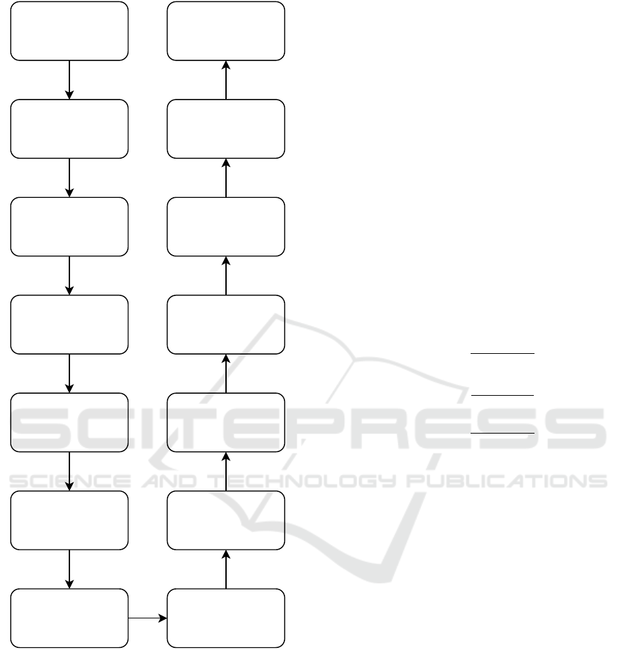
Combine the chosen
channels
Apply OTSU
thresholding
to the chosen
channels
Apply Saliency on the
chosen channels
Get the 4 luminance
invariant images and
the A channel
YCbCr to BGR
C1C2C3 to YCbCr
Extract Shadows from
HSV
Gamma Correction
Input Frame
Apply OTSU
thresholding
to the combined
image
Extract contours
Remove contour
noise
BGR to C1C2C3
Use the extracted
shadows to correct
the YCbCr
Figure 1: The proposed pipeline flow.
To be able to efficiently extract the drivable area,
shadows had to be removed based only on CV-IM,
multiple factors had to be taken into consideration to
ensure the algorithm accuracy is as high as possible.
The correct detection and extraction of road edges in-
dependent of color have to be robust. The shadows
have to be handled without losing other vital spatial
information such as the drivable area edges. Rapid
changes in illumination also have to be taken care of
dynamically to stabilize the performance of the sys-
tem during illumination transitions. The following
sections discuss the pipeline flow in detail.
3.1 Gamma Correction
Given the images captured from the camera are in a
gamma compressed state, Gamma decompression is
applied on the input images to be able to apply the
shadow removal techniques and get the best possible
result. Without correction, the shadows in the image
are darker than they seem. An example can be seen in
(a) and (b) in 3. In other words, the gamma correction
reveals better details of the areas occluded inside the
shadow regions.
3.2 c1c2c3
Following the gamma decompression, the images
were converted from RGB color to c1c2c3 color
space, as defined in (Gevers and Smeulders, 1999) as
in 1, 2 and 3 and shown in (c1) in 3.
c1 = arctan(
R
MAX(G, B)
) (1)
c2 = arctan(
G
MAX(R, B)
) (2)
c3 = arctan(
B
MAX(R, G)
) (3)
Where the R, G and B are the red, green and blue
channels respectively. The denominators of c1, c2
and c3 are based on the channel with the larger sum-
mation. The c1c2c3 was chosen as it reduces the vari-
ance in luminance information in the image which re-
duces the shadow intensities significantly and helps
improve the overall result of proposed pipeline.
3.3 YCbCr Correction
For further refinement, the gamma corrected image is
converted to the HSV color space to apply the shadow
detection technique used in (Mishra and Chourasia,
2017). This method was found to be crucial to de-
tect the areas which are guaranteed to contain shad-
ows. A sample result can be seen in Figure 3 (d2).
After applying this technique, a simple pixel classi-
fication is applied channel wise to the YCbCr image
representation of the c1c2c3 image. This step is ap-
plied to ensure that most of the shadow cells are taken
into account to extract a corrected median value for
the shadow and shadowless regions in each channel.
Algorithm 1 contains the steps for the shadow mask
expansion and channel inpainting.
The algorithm starts by taking the lower half of
the Hue-Intensity image and for each channel of the
ICAART 2021 - 13th International Conference on Agents and Artificial Intelligence
762
Algorithm 1: Shadow neutralization steps.
1 Smask
Lower
= Smask[H*0.5:,:]
2 k = 0
3 while k < 3 do
4 Median
shadow
k
= median(
C
k
[Smask
Lower
> 0] )
5 Median
shadowless
k
= median(
C
k
[Smask
Lower
== 0] )
6 Shadow
loc
= ( abs(C
k
- Median
shadow
k
) ¡
abs(C
k
- Median
shadowless
k
) )
7 Smask
k
= Smask
Lower
8 Smask
k
[Shadow
loc
] = 255
9 Median
new
shadow
k
= median(
C
k
[Smask
k
> 0] )
10 Median
new
shadowless
k
= median(
C
k
[Smask
k
== 0] )
11 Median
di f f
k
= Median
new
shadow
k
-
Median
new
shadowless
k
12 C
k
[Smask
k
> 0] = C
k
[Smask
k
> 0] +
Median
di f f
k
13 k = k + 1
14 end
YCbCr image, the median value of the shadow re-
gion and the non-shadow region are extracted. Fur-
thermore, classification based on the extracted median
values is applied channel-wise to expand the shadow
mask. Finally, the extracted shadow mask region is
altered by the difference between the median of the
shadow and the non-shadow regions.
The YCbCr color space was specially chosen as
it separates the luma (Y ) representing the brightness
of the image from the chrominance color information
represented in Cb and Cr.
3.4 Channels Selection
After correcting the YCbCr image, it was converted
to RGB color space as in Figure 3 (f), then the LAB
and HSV images are extracted.
Following the initial approach suggested in (Ka-
tramados et al., 2009), the following channels were
selected from the paper:
1. The Mean-Chroma as defined in (Katramados
et al., 2009) and seen in equation 3.4 and in Figure
3 (g).
2. The Saturation-based texture as defined in (Katra-
mados et al., 2009).
3. The Chroma-based texture as defined in (Katra-
mados et al., 2009).
In addition, the edges channel obtained by applying
the Sobel operator on the A channel from the LAB
color space was also added to the selected channels.
m
c
=
2A +Cb +Cr
4
(4)
Where the A is the A channel of the LAB color space.
The Cb and Cr are the blue and red chrominance from
the YCbCr color space.
3.5 Saliency Application with OTSU
Thresholding
After selecting the channels, fine grained Saliency
proposed in (Montabone and Soto, 2010), was com-
puted for each channel followed by applying the
OTSU thresholding approach (Otsu, 1979). This
combination is near to (Fan et al., 2017) with the dif-
ference of using the fine-grained Saliency to preserve
the obtained spatial information of the image as in (h)
in 3. Furthermore, the 4 mentioned resultant chan-
nels were combined and the OTSU thresholding was
applied once more on the combined image to classify
the drivable and non-drivable regions.
3.6 Contour Validation
As a further step to refine the extracted drivable area,
the object contours with small areas detected in the
image produced from the OTSU thresholding were
removed using the contour extraction (Suzuki et al.,
1985) as seen in (k) in 3.
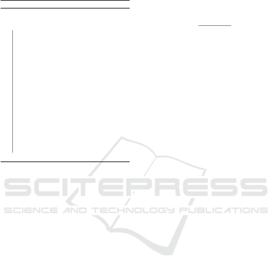
3.7 Deep Learning based Approach
based on the Proposed Pipeline
To verify the performance improvement that the pro-
posed pipeline produces compared to the standard
grayscale image, tests using DL were applied. The
output image from the pipeline before applying the
saliency and the OTSU method was used as an in-
put to a semantic segmentation DL model to see how
the proposed pipeline affects the performance of DL
models that can be used for drivable area segmenta-
tion. The used model is the U-Net depicted in Figure
2.
Drivable Area Extraction based on Shadow Corrected Images
763
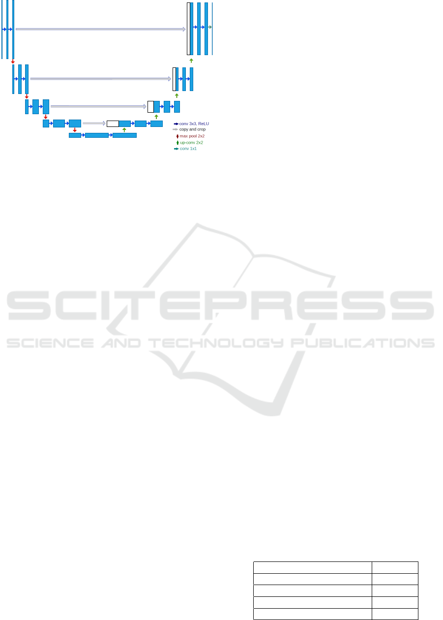
Figure 2: An example showing the structure of the U-Net
model. Each blue rectangle corresponds to a feature map.
The arrows denote different operations as seen in the leg-
end in the image. Red arrows denote maxpooling down-
sampling, green arrows denote upsampling, the blue arrows
denote the convolutional layers and the gray arrows repre-
sent the (Qiang et al., 2019).
4 PERFORMANCE EVALUATION
4.1 Setup
4.1.1 Hardware
To run the proposed pipeline, a laptop with an i7-
6700HQ processor running Ubuntu 18.04 and a Log-
itech C920 camera were used to conduct the tests. The
system was placed on the autonomous golf-car proto-
type of the SDC lab at the GUC.
4.1.2 Software Parameters
The gamma correction coefficient used was manu-
ally set to 2.2 as widely used computers compress the
gamma by 0.45. The used U-Net input image was
set to 256x256 to reduce the computing power needed
and make the code run with sufficient fps for closed
campus situations.
For the U-Net, An Adam optimizer with binary
cross-entropy loss was used for training. Further-
more, the dataset used consist of 246 images taken
from the autonomous golf-car prototype of the SDC
lab inside the GUC. The data was split into 90%-10%
for training and testing respectively. A batch size of
32 was used for 200 epochs. However, early stopping
was applied to prevent the model from over-fitting.
4.2 Experiments
The proposed algorithm was tested on images at dif-
ferent times of the day at: 10 am, 12 pm, 4 pm
and 7pm (sunset was around 6:30 pm during these
tests) at different locations on the GUC campus. This
was conducted to measure the performance related
to multiple illumination conditions as well as differ-
ent shadow intensities. One of the test sequences
was taken while manually driving around the football
court track on campus as seen in Figure 6 at an av-
erage speed of 7 kph. Other sequences were taken
around the campus streets at different times of the day.
For the trained DL models of the U-Net, the ac-
curacy was used to measure the performance. The
model architecture was tested on the gray scaled im-
age after applying the gamma correction as well as
RGB images to compare the performance based on
the proposed pipeline image with the normal image
without the pipeline. For the CV-IM, the final image
was inverted and then the accuracy metric was also
applied based on a comparison with the ground truth.
4.3 Results and Discussion
After conducting the previously mentioned tests on
different images, the following results were observed.
For the U-Net training, it was observed during train-
ing that the RGB image converged first with no im-
provement throughout the first 15 epochs, the normal
gray scaled image converged afterwards, and finally
the image from the proposed pipeline converged the
last. Furthermore, the results of training on the re-
sultant image from the pipeline surpassed the normal
gray scale images which exceeded the results of pre-
dicting on the RGB images. The outcome of using
the resultant image from the proposed approach had
an accuracy higher than that of the result of using the
normal gray scale image which was in turn more than
the RGB image. Qualitative results of the U-Net can
be seen in Figure 4 based on the resultant pipeline im-
age and 5 based on the normal gray scale image.
As seen in Figures 4 and 5, the output from the
proposed pipeline significantly improved the predic-
tion of the U-Net. For further testing to prove the ef-
fect of the proposed pipeline, the inverted results of
using the full pipeline were also calculated without
utilizing DL. A binary accuracy metric was used to
calculate the pixel-wise accuracy of the segmentation.
The following table shows the results of using the four
segmentation methods discussed on a separate testing
set of images.
Table 1.
used method accuracy
UNET on resultant image 91%
proposed pipeline 82%
UNET on gray scale image 75%
UNET on RGB image 69%
ICAART 2021 - 13th International Conference on Agents and Artificial Intelligence
764
(a)
(i)
(h)
(g)
(b)
(k)(j)
(c2)
(c1)
(d1)
(d2)
(f)
(e)
Figure 3: A visual representation of the flow of the proposed algorithm. The input image (a) read from the camera is given
to the pipeline. The image is first gamma corrected (b) and then in a parallel step, a copy of the image is converted c1c2c3
image (c1) and another copy is converted to the HSV color space (c2) and the shadow mask is extracted by the Hue-Intensity
ratio for the bottom half of the image. Furthermore, the extracted shadow mask is used with the YCbCr representation (d1) of
the c1c2c3 image for the shadow mask expansion (e) to improve the shadow removal. The resultant corrected YCbCr image
was converted to RGB color space to get the corrected HSV and LAB images alongside the corrected YCbCr. The 4 combined
channels are then extracted (g) Mean-Chroma, Saturation-based texture, Chroma-based texture and the Sobel operator on the
A channel from the LAB color space left to right respectively. Furthermore, Saliency and OTSU thresholding are applied on
the 4 chosen channels (h) and combined (i). Finally, a final OTSU thresholding step is applied to get the obstacles in white
and the drivable area in black (k).
From the table, it can be observed that using DL is
still better with the use of the resultant image. How-
ever, the proposed pipeline alone surpasses the use of
DL on the normal gray scale images as well as us-
ing the RGB image. Figure 7 shows a comparison of
the different approaches to the same input image. Its
worth noting that the results of the better approaches
were used hence the RGB image was left out.
Moreover, the computation time comparison was
also held. The use of the proposed pipeline alone ex-
ecuted in and average of 16 fps compared to the DL
which ran at around 6 fps.
For the results of the given scenarios, the algo-
rithm was able segment the drivable area at different
times of the day successfully and still was able to per-
form robustly as shown in Figure 7.
Drivable Area Extraction based on Shadow Corrected Images
765
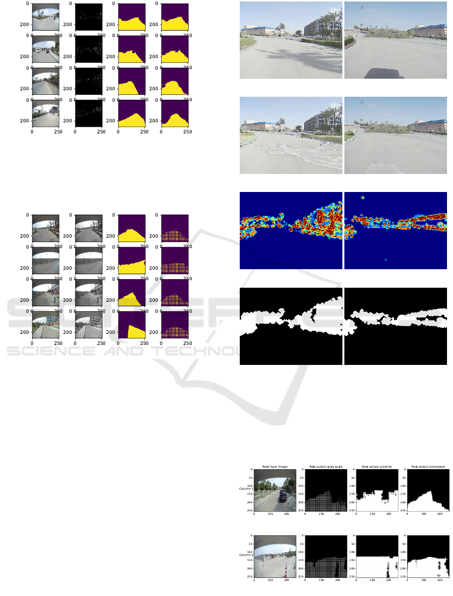
Figure 4: An example of the results of drivable area seg-
mentation using the resultant image. The first column is the
original image without pre-processing, the second column
shows the image after the pre-processing step, the third col-
umn is the ground truth, and finally the fourth column is
model’s prediction.
Figure 5: An example of the results of drivable area seg-
mentation using the gray scale image. The first column is
the original image without pre-processing, the second col-
umn shows the image after the pre-processing step, the third
column is the ground truth, and finally the fourth column is
model’s prediction.
Given that the main aim of the algorithm is to
segment the drivable area at certain situations tackle
limited situations, the proposed system outperforms
previous systems with similar use of sensors. This
is mainly due to the shadow removal pre-processing
step that proved to be robust in the mentioned sit-
uations in the paper. With additional work, the al-
gorithm can be a solid base for further development
aiming at more efficient segmentation and detection
algorithms for autonomous vehicles.
Limitations
The proposed algorithm has few limitations. Running
the proposed algorithm at night is not currently pos-
sible due to the insufficient lighting conditions. Fur-
thermore, if the scene contains pavements and roads
(a) (b)
(c) (d)
(e) (f)
(g) (h)
Figure 6: An example with 2 frames around the football
court. Figures 6a and 6b show the gamma corrected image,
Figures 6c and 6d show the inpainted image, Figures 6e and
6f show The JET color-map of the combined image and fi-
nally Figures 6g and 6h show The extracted drivable area.
In this test, the prototype golf-car was moving at an average
of 7+ kph.
Figure 7: Comparison for the approaches’ results.
with near identical color levels, the algorithm fails to
segment the drivable area correctly due to the lack of
ICAART 2021 - 13th International Conference on Agents and Artificial Intelligence
766

proper edges to base the segmentation on.
5 CONCLUSIONS
This paper proposed a monocular vision based driv-
able area segmentation pipeline that was able to de-
tect the drivable area with and without the presence
of shadows in the scene in different situations without
any additional sensors. The CV-IM pipeline proved
to be robust and surpassed a DL network in the pro-
cess. In addition, the use of the output image from
the pipeline as an input to the DL model significantly
improved the prediction compared to the normal gray
scale image. Moreover, the system is independent
from the use of any maps and is a plug-and-play one.
Future work can include making the pipeline more ro-
bust to work in more challenging situations as well as
adding more modules such as object detection.
REFERENCES
Bai, M., Mattyus, G., Homayounfar, N., Wang, S., Lak-
shmikanth, S. K., and Urtasun, R. (2018). Deep
multi-sensor lane detection. In IEEE/RSJ Interna-
tional Conference on Intelligent Robots and Systems
(IROS), pages 3102–3109.
Fan, H., Xie, F., Li, Y., Jiang, Z., and Liu, J. (2017).
Automatic segmentation of dermoscopy images using
saliency combined with otsu threshold. Computers in
biology and medicine, 85:75–85.
Gevers, T. and Smeulders, A. W. (1999). Color-based object
recognition. Pattern recognition, 32(3):453–464.
Gurghian, A., Koduri, T., Bailur, S. V., Carey, K. J., and
Murali, V. N. (2016). Deeplanes: End-to-end lane po-
sition estimation using deep neural networksa. In Pro-
ceedings of the IEEE Conference on Computer Vision
and Pattern Recognition Workshops, pages 38–45.
Haque, M. R., Islam, M. M., Alam, K. S., Iqbal, H., and
Shaik, M. E. (2019). A computer vision based lane
detection approach. International Journal of Image,
Graphics and Signal Processing, 11(3):27.
Hata, A. and Wolf, D. (2014). Road marking detection us-
ing lidar reflective intensity data and its application to
vehicle localization. In 17th International IEEE Con-
ference on Intelligent Transportation Systems (ITSC),
pages 584–589.
Hou, Y. (2019). Agnostic lane detection. arXiv preprint
arXiv:1905.03704.
Katramados, I., Crumpler, S., and Breckon, T. P. (2009).
Real-time traversable surface detection by colour
space fusion and temporal analysis. In International
Conference on Computer Vision Systems, pages 265–
274. Springer.
Kim, Z. (2008). Robust lane detection and tracking in chal-
lenging scenarios. IEEE Transactions on Intelligent
Transportation Systems, 9(1):16–26.
Levi, D., Garnett, N., Fetaya, E., and Herzlyia, I. (2015).
Stixelnet: A deep convolutional network for obsta-
cle detection and road segmentation. In BMVC, pages
109–1.
Miksik, O., Petyovsky, P., Zalud, L., and Jura, P. (2011).
Robust detection of shady and highlighted roads for
monocular camera based navigation of ugv. In 2011
IEEE International Conference on Robotics and Au-
tomation, pages 64–71. IEEE.
Mishra, A. and Chourasia, B. (2017). Modified hue over
intensity ratio based method for shadow detection and
removal in arial images. INTERNATIONAL JOUR-
NAL OF ADVANCED ENGINEERING AND MAN-
AGEMENT, 2:101.
Montabone, S. and Soto, A. (2010). Human detection using
a mobile platform and novel features derived from a
visual saliency mechanism. Image and Vision Com-
puting, 28(3):391–402.
Neto, A. M., Victorino, A. C., Fantoni, I., and Ferreira, J. V.
(2013). Real-time estimation of drivable image area
based on monocular vision. In IEEE Intelligent Ve-
hicles Symposium Workshops (IV Workshops), pages
63–68.
Otsu, N. (1979). A threshold selection method from gray-
level histograms. IEEE Transactions on Systems,
Man, and Cybernetics, 9(1):62–66.
Qiang, Z., Tu, S., and Xu, L. (2019). A k-dense-unet
for biomedical image segmentation. In International
Conference on Intelligent Science and Big Data Engi-
neering, pages 552–562. Springer.
Suzuki, S. et al. (1985). Topological structural analy-
sis of digitized binary images by border following.
Computer vision, graphics, and image processing,
30(1):32–46.
Drivable Area Extraction based on Shadow Corrected Images
767
