Compiling Possibilistic Networks to Compute Learning Indicators
Guillaume Petiot
CERES, Catholic Institute of Toulouse, 31 rue de la Fonderie, 31068, Toulouse, France
Keywords:
Uncertain Gates, Compiling Possibilistic Networks, Possibility Theory, Education, Decision Making.
Abstract:
University teachers, who generally focus their interest on pedagogy and students, may find it difficult to
manage e-learning platforms which provide learning analytics and data. But learning indicators might help
teachers when the amount of information to process grows exponentially. The indicators can be computed by
the aggregation of data and by using teachers’ knowledge which is often imprecise and uncertain. Possibility
theory provides a solution to handle these drawbacks. Possibilistic networks allow us to represent the causal
link between the data but they require the definition of all the parameters of Conditional Possibility Tables.
Uncertain gates allow the automatic calculation of these Conditional Possibility Tables by using for example
the logical combination of information. The calculation time to propagate new evidence in possibilistic net-
works can be improved by compiling possibilistic networks. In this paper, we will present an experimentation
of compiling possibilistic networks to compute course indicators. Indeed, the LMS Moodle provides a large
scale of data about learners that can be merged to provide indicators to teachers in a decision making system.
Thus, teachers can propose differentiated instruction which, better corresponds to their student’s expectations
and their learning style.
1 INTRODUCTION
Modeling indicators based on expert knowledge are
hard to perform because human description is often
vague. Possibility theory, introduced by L. A. Zadeh
(Zadeh, 1978), is a solution to this problem of un-
certainty which appears during knowledge modeling.
Moreover, the causal link between the data can be
modeled by using the possibilistic network (Benfer-
hat et al., 1999). The latter is an adaptation of the
Bayesian Network (Pearl, 1988; Neapolitan, 1990) to
possibility theory. In the possibilisic network each
variable is attached to a Conditional Possibility Table.
The number of parameters to elicit in a CPT grows
exponentially depending proportionally on the num-
ber of parents. So a solution can be to use uncertain
logical gates between the variables in order to com-
pute automatically the CPT instead of eliciting all pa-
rameters. This time-saving solution allows us to fix
the problem of unknown variables which are too dif-
ficult to extract from complex systems. The addition
of a variable called leakage variable leads to a new
model. There is a large set of available connectors
from behavior severe to indulgent. The variables are
often qualitative as in (Dubois et al., 2015) but to use
uncertain gates we have to encode the modalities into
numerical values.
Another problem is the computation time of the
propagation of evidence in possibilistic networks.
There are several existing solutions with exact in-
ference or approximative inference. For example
forward-chaining, message passing in junction tree,
etc. But in our study we propose to experiment a new
approach which is more efficient. Indeed, it is possi-
ble to perform the compiling of the possibilistic net-
work as for Bayesian networks (Park and Darwiche,
2002) to improve the computation time.
In this paper, we would like to perform an ex-
perimentation of indicator calculation by using uncer-
tain gates and compiling possibilistic networks. Sev-
eral studies were performed in order to improve peda-
gogy and understand students and their learning style
(Huebner, 2013; Baker and Yacef, 2009; Bousbia
et al., 2010). These researchers made use of Bayesian
networks, neural networks, support vector machines.
They often tried to detect a student at the risk of drop-
ping out or failing at the examination.
Our approach study is based on an existing dataset
built from Moodle logs for a course of spread-
sheet and some external information such as atten-
dance and results at the examination. This dataset is
anonymized. We can extract from Moodle the results
of the quiz, the sources consulted, etc. The knowl-
edge about the indicators is provided by teachers and
Petiot, G.
Compiling Possibilistic Networks to Compute Learning Indicators.
DOI: 10.5220/0010238001690176
In Proceedings of the 13th International Conference on Agents and Artificial Intelligence (ICAART 2021) - Volume 2, pages 169-176
ISBN: 978-989-758-484-8
Copyright
c
 2021 by SCITEPRESS – Science and Technology Publications, Lda. All rights reserved
169

extracted from the data by data mining as in (Petiot,
2018).
The goal of this paper, is to compute course in-
dicators by using teachers’ knowledge. To do this,
we will first present possibility theory and uncertain
gates. Then we will focus on the compiling of pos-
sibilistic networks and finally we will present our re-
sults.
2 UNCERTAIN GATES
Uncertain gates are an analogy of noisy gates in pos-
sibility theory, developed in 1978 by L.A. Zadeh
(Zadeh, 1978). In this theory, imprecise and uncer-
tain knowledge can be modeled by a possibility dis-
tribution π. We can define the possibility measure Π
and the necessity measure N from P(Ω) in [0,1] as the
authors in (Dubois and Prade, 1988). The possibility
measure is defined as follows:
∀A ∈ P(Ω), Π(A) = sup
x∈A
π(x)
(1)
The necessity measure can be defined as follows:
∀A ∈ P(Ω), N(A) = 1 − Π(¬A) = in f
x/∈A
1 − π(x)
(2)
Possibility theory is not additive but maxitive:
∀A,B ∈ P(X), Π(A ∪ B) = max(Π(A),Π(B)).
(3)
We can compute the possibility of the variable A given
the variable B by using the conditioning proposed
by E. Hisdal (Hisdal, 1978) and generalized by D.
Dubois and H. Prade (Dubois and Prade, 1988):
Π(A|B) =

Π(A,B) if Π(A,B) < Π(B),
1 if Π(A,B) = Π(B).
(4)
Possibilistic networks (Benferhat et al., 1999; Borgelt
et al., 2000) can be defined by using the factoring
property. We propose the following definition:
Definition 2.1. The factoring property can be defined
from the joint possibility distribution Π(V ) for a Di-
rectional Acyclic Graph (DAG) G = (V, E) where V is
the set of Variables and E the set of edges between the
variables. Π(V ) can be factorized toward the graph G:
Π(V ) =
O
X∈V
Π(X/Pa(X)).
(5)
The function Pa(X) returns the parents of the variable
X.
There are two kinds of possibilistic networks: min-
based possibilistic networks that are qualitative pos-
sibilistic networks where
N
is the function min, and
product-based possibilistic networks that are quanti-
tative possibilistic networks where
N
is the product.
In this research, we will use a min-based possibilistic
network because we have chosen to compare the pos-
sibilistic values instead of using an intensity scale in
[0,1].
Uncertain logical gates were proposed for the first
time by the authors of (Dubois et al., 2015). They are
based on the Independence of Causal Influence and
use a model to represent uncertainty. This model is
built by introducing an intermediate variable Z
i
be-
tween a set of causal variables X
1
,...,X
n
and an effect
variable Y . This allows us to represent two behaviors:
inhibitors and substitute. The inhibitors can be de-
fined if a cause is met and the effect variable Y is not
produced. The substitute can be defined if a cause is
not met and the variable Y is produced. In this model,
there is a deterministic function f which combines the
influences of the variables Z
i
s: Y = f (Z
1
,...,Z
n
). The
leaky model is derived from the previous model by
adding a leakage variable Z
l
which represents the un-
known knowledge. The possibilistic model with the
ICI is the following:
Figure 1: Possibilistic model with ICI.
This model, presented by the authors (Dubois et al.,
2015), leads to the following equation:
π(y|x
1
,...,x
n
) = max
z
1
,...,z
n
,z
l
:y= f (z
1
,...,z
n
,z
l
)
n
O
i=1
π(z
i
|x
i
) ⊗π(z
l
)
(6)
The ⊗ is the minimum and ⊕ is the maximum. There
are several possible functions f , for example AND,
OR, NOT, INV, XOR, MAX, MIN, MEAN, linear
combination, etc.
In order to generate the CPT we have to compute
the above equation. We have to define π(Z
i
|X
i
), π(Z
l
),
and the function f . In our experimentation we have
three ordered levels of intensity: low, medium and
high. We propose to encode the modality by the fol-
lowing intensity levels as in (Dubois et al., 2015): 0
for low, 1 for medium and 2 for high. The following
table illustrates an example:
ICAART 2021 - 13th International Conference on Agents and Artificial Intelligence
170

Table 1: Possibility table for 3 ordered states.
π(Z
i
|X
i
) x
i
= 2 x
i
= 1 x
i
= 0
z
i
= 2 1 s
2,1
i
s
2,0
i
z
i
= 1 κ
1,2
i
1 s
1,0
i
z
i
= 0 κ
0,2
i
κ
0,1
i
1
In the above table, κ represents the possibility that an
inhibitor exists if the cause is met and s
i
the possibil-
ity that a substitute exists when the cause is not met.
If a cause of weak intensity cannot produce a strong
effect, then all s
i
= 0. So there are 6 parameters at the
most per variable and 2 parameters for π(Z
l
). Another
constraint is that κ
1,2
i
≥ κ
0,2
i
.
In our study we will use for the function f the
function MIN and MAX leading to the connectors
uncertain MIN (⊥) and uncertain MAX (>) as pro-
posed by Dubois et al. (Dubois et al., 2015). We will
also use a weighted average function (WAVG) and a
MYCIN Like connector (~) as described in (Petiot,
2018). The function f must have the same domain
as the variable Y . We can see that the connectors un-
certain MIN and uncertain MAX satisfy this property.
Nevertheless, the weighted average function can re-
turn a value outside the domain of Y . We propose to
combine the result of the weighted average function
g(z
1
,...,z
n
) = ω
1
z
1
+ ... + ω
n
z
n
with a scaling func-
tion f
s
which returns a value in the domain of Y . The
parameters ω
i
are the weights of the weighted aver-
age. Finally, we have f = f
s
◦ g. If (ε
0
,ε
1
,...,ε
m−1
)
are the m ordered states of Y then the function f
s
can
be for example:
f
s
(x) =







ε
0
if x ≤ θ
0
ε
1
if θ
0
< x ≤ θ
1
.
.
.
.
.
.
ε
m−1
if θ
m−2
< x
(7)
The parameters θ
i
allow us to adjust the behaviour
of f
s
. The function g has n parameters which are the
weights w
i
of the linear combination and n arguments.
If all weights are equal to
1
n
, then we calculate the
average of the intensities. If ∀
i∈[1,n]
ω
i
= 1, then we
make the sum of the intensities (connector
∑
).
3 COMPILING THE JUNCTION
TREE OF A POSSIBILISTIC
NETWORK
The knowledge of the indicators is represented by a
possibilistic network. The propagation of evidence in
this possibilistic network will lead to a possibility and
a certainty measure.
To perform the propagation of evidence in the pos-
sibilistic network we propose at first to compile the
junction tree of a possibilistic network. The junc-
tion tree is composed of cliques and separators. The
cliques are extracted by using the Kruskal algorithm
(Kruskal, 1956) after the generation of the moral
graph and the triangulated graph (Kjaerulff, 1994).
The same reasoning as in compiling Bayesian net-
works (Darwiche, 2003) is used. We have adapted A.
Darwiche’s algorithm for the junction tree (Park and
Darwiche, 2002) of a Bayesian network to possibilis-
tic networks.
Indeed, possibilistic networks can be transformed
into a function with two kind of variables: evidence
indicators and network parameters. For all instantia-
tions of a variable X = x we define an evidence indi-
cator λ
x
. Similarly, for all network CPT parameters
of π(X |U ), we define a parameter θ
x|u
where u is an
instantiation of U , the parents of the variable X and x
an instantiation of the variable X.
The function f can be computed by combining at
first all evidence indicators and network parameters
consistent with the instantiation by using the operator
⊗. Then, we perform a combination of all the previ-
ous results by using the operator ⊕.
Definition 3.1. If P is a possibilistic network, V = v
the instantiations of the variables of the possibilistic
networks and U = u the consistent instantiations of
the parents of a variable X with the instantiation X =
x, then the function f of P is:
f =
M
v
O
xu∼v
λ
x
⊗ θ
x|u
(8)
In the above formula xu denotes the instantiation of
the family of X and its parents U compatible with the
instantiation v. The operator
L
can be the function
maximum and
N
the function minimum.
We can study, as an example, the following possibilis-
tic network:
Table 2: Example of the possibilistic network A → B → C.
A B
true true θ
b|a
true false θ
¯
b|a
false true θ
b| ¯a
false false θ
¯
b| ¯a
A
true θ
a
false θ
¯a
B C
true true θ
c|b
true false θ
¯c|b
false true θ
c|
¯
b
false false θ
¯c|
¯
b
Compiling Possibilistic Networks to Compute Learning Indicators
171

In this case the function f is:
f = λ
a
⊗ λ
b
⊗ λ
c
⊗ θ
a
⊗ θ
b|a
⊗ θ
c|b
⊕λ
a
⊗ λ
b
⊗ λ
¯c
⊗ θ
a
⊗ θ
b|a
⊗ θ
¯c|b
...
⊕λ
¯a
⊗ λ
¯
b
⊗ λ
¯c
⊗ θ
¯a
⊗ θ
¯
b| ¯a
⊗ θ
¯c|
¯
b
(9)
Definition 3.2. If the evidence e is an instantiation of
variables then we have the property f (e) = π(e).
Let us consider the following example:
Table 3: Example of the possibilistic network A → B.
A B
true true 1
true false 0.2
false true 0.1
false false 1
A
true 1
false 0.1
If the evidence is ¯a, then we obtain λ
a
= 0, λ
¯a
= 1,
λ
b
= 1, λ
¯
b
= 1 and the computation of f (e) is: f ( ¯a) =
f (λ
a
= 0,λ
¯a
= 1,λ
b
= 1,λ
¯
b
= 1) = θ
¯a
⊗ θ
b| ¯a
⊕ θ
¯a
⊗
θ
¯
b| ¯a
= 0.1 ⊗ 0.1 ⊕ 0.1 ⊗ 1.0 = 0.1. The evaluation of
f leads us to compute π(e).
We can compute the possibility of a variable X
given the evidence e:
π(x|e) =
(
π(x,e) if π(x,e) < π(e),
1 if π(x,e) = π(e).
(10)
If the variable X has n states and x is one of its
states, and if X is not in the evidence e then π(x, e) =
f (e,1
λ
x
) with 1
λ
x
= (λ
x
1
= 0, ...,λ
x
= 1, ...,λ
x
n
= 0).
For example, 1
λ
¯a
= (λ
a
= 0,λ
¯a
= 1). We have an-
other case if X is in e called Evidence Retraction in
probability theory (Darwiche, 2003). In possibility
theory the Evidence Retraction leads us to compute
π(x|e − X).
If the number of variables is too high, the com-
puting of possibilities becomes too complex. So it is
interesting to compile the possibilistic network by us-
ing a MIN-MAX circuit as in (Raouia et al., 2010).
This optimization allows us to reduce memory used
and computation time. There are several approaches
for compiling the function f into a MIN-MAX circuit.
The leaves of the MIN-MAX circuit are the parame-
ters λ and θ and the nodes are the operators ⊗ and ⊕.
We present an example of a MIN-MAX circuit in the
following figure:
Figure 2: MIN-MAX circuit of the example.
We have chosen to perform the factorisation of the
function f and then to use the junction tree method.
To compile a Bayesian network under evidence, we
generate an arithmetic circuit and we differentiate the
circuit in order to obtain all posterior probabilities
p(x|e). The differentiation is very easy with the arith-
metic circuit in probability theory.
Definition 3.3. We obtain the arithmetic circuit f
0
of
a MIN-MAX circuit f by replacing the ⊗ by the mul-
tiplications and the ⊕ by additions.
We propose to encode the MIN-MAX circuit into
an arithmetic circuit. Then we will deduce the propa-
gation algorithm for the arithmetic circuit. Finally, we
will replace in the algorithm the additions by ⊕ and
the multiplications by ⊗ in order to apply the algo-
rithm to a MIN-MAX circuit. In the following figure
we present an example of our encoding:
(a) MIN-MAX circuit.
(b) Arithmetic circuit.
Figure 3: Arithmetic circuit of a MIN-MAX circuit.
ICAART 2021 - 13th International Conference on Agents and Artificial Intelligence
172

We can differentiate the polynomial
∂ f
0
∂λ
x
. In the exam-
ple of Table 3, we obtain the following function:
f = λ
a
⊗ θ
a
⊗ (λ
b
⊗ θ
b|a
⊕ λ
¯
b
⊗ θ
¯
b|a
)
⊕λ
¯a
⊗ θ
¯a
⊗ (λ
b
⊗ θ
b| ¯a
⊕ λ
¯
b
⊗ θ
¯
b| ¯a
)
(11)
After the transformation we obtain the following
polynomial:
f
0
= λ
a
θ
a
(λ
b
θ
b|a
+ λ
¯
b
θ
¯
b|a
) + λ
¯a
θ
¯a
(λ
b
θ
b| ¯a
+ λ
¯
b
θ
¯
b| ¯a
) (12)
For example, if we suppose that e = b then f
0
(e) =
f
0
(λ
b
= 1;λ
¯
b
= 0;λ
a
= 1;λ
¯a
= 1). To compute π(a,e)
we must at first compute
∂ f
0
(e)
∂λ
a
because a is not in e.
We obtain the following result:
∂ f
0
(e)
∂λ
a
= θ
a
θ
b|a
(13)
To obtain π(a,e) we must replace the additions by ⊕
and the multiplications by ⊗ in the above equation,
which gives the following result:
π(a,e) = θ
a
⊗ θ
b|a
(14)
We propose to build the MIN-MAX circuit of a junc-
tion tree obtained from a possibilistic network. We
must first select a root node which is the result of f ,
then we add a ⊕ node for each instantiation of a sep-
arator and a ⊗ node for each instantiation of a cluster.
We have only one node λ
x
for each instantiation of a
variable X and one node θ
x|v
for each instantiation of
the nodes X and its parents V. The children of the out-
put node f are the ⊗ nodes of the root cluster. The
children of ⊕ nodes are compatible nodes generated
by the child clusters and the children of a ⊗ node are
compatible nodes generated by the child separators.
Each variable and λ are affected to only one cluster.
If we consider the example B ←− A −→ C we can
compute the MIN-MAX circuit of the junction tree as
follows:
Figure 4: MIN-MAX circuit of a junction tree.
In this figure, the function φ performs the evaluation
of the cluster compatible with the instantiation of the
separator.
We propose now to differentiate the arithmetic cir-
cuit f
0
of a MIN-MAX circuit f . If v is the current
node and p is the parents of v, then we can compute
∂ f
0
∂v
by using the chain rule:
∂ f
0
∂v
=
∑
p
∂ f
0
∂p
∂p
∂v
(15)
If the parent p has n other children v
i
different from
the node v, there are several cases to discuss:
• If v is the first node then
∂ f
0
∂v
= 1.
• If p is an addition node then
∂p
∂v
=
∂(v+
∑
n
i=1
v
i
)
∂v
= 1
• If p is a multiplication node then
∂p
∂v
=
∂(v
∏
n
i=1
v
i
)
∂v
=
∏
n
i=1
v
i
As a result, we obtain the following recursive algo-
rithm to evaluate the MIN-MAX circuit of a junction
tree by changing the multiplication by ⊗ and addi-
tions by ⊕:
1. Upward-pass: compute the value of the node v
and store it in u(v);
2. If v is the root then set d(v) = 1 else set d(v) = 0;
3. Downward-pass: for each parent p of the node v
compute d(v) as follows:
(a) if p is a node ⊕:
d(v) = d(v)
M
d(p) (16)
(b) if p is a node ⊗:
d(v) = d(v)
M
"
d(p)
O
"
n
O
i=1
u(v
p
i
)
##
(17)
The nodes v
p
i
are the other children of p;
To evaluate the indicators, we must perform several
processing operations. The first one is to compile the
junction tree of the possibilistic network. Then we
perform the initialization of evidence before apply-
ing the recursive algorithm. We can compute for each
state of an indicator a possibility measure and a ne-
cessity measure.
4 EXPERIMENTATION
4.1 Presentation
In our experimentation, we used an existing
anonymized dataset for a Spreadsheet course at bach-
elor level proposed in face-to-face learning enriched
by an online supplement on Moodle. This dataset was
built by gathering all data of logs in a table. Then a
process of anonymization was performed. For exam-
ple, we use the data of Moodle, such as quiz results,
Compiling Possibilistic Networks to Compute Learning Indicators
173

sources consulted, ... and external data such as atten-
dance, groups,... The quiz questions were categorized
by skills. When the data were missing, we performed
an imputation of these data by an iterative PCA (Au-
digier et al., 2015). The knowledge about the indica-
tors was provided by teachers and extracted from the
data by data mining. To represent the knowledge we
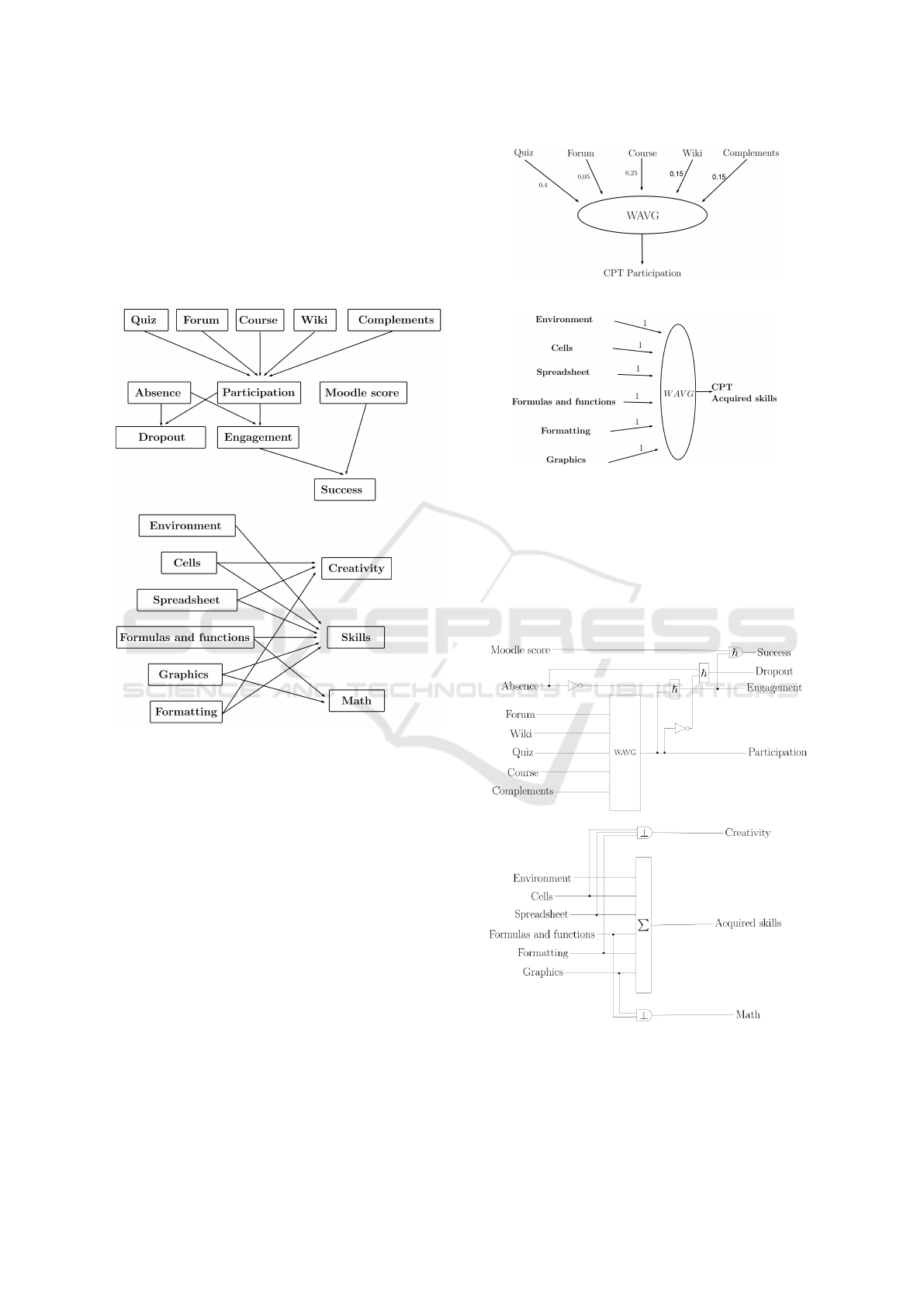
have chosen to use a DAG:
Figure 5: Modeling of knowledge by a DAG.
The qualitative variables have 3 ordered modalities
(low, medium, high) encoded with the numerical val-
ues (0,1,2). The description of the indicators by teach-
ers is often imprecise so we used a possibility distri-
bution to represent each state of a variable. Then, pos-
sibilistic networks can be used to compute the indica-
tors. To do this we need to define all CPTs. To avoid
the eliciting of all the parameters, we used uncertain
gates leading to the computation of all the CPTs.
We merged information about the sources con-
sulted in Moodle to build an indicator of participation
which takes into account their importance. We used
the WAVG connector. The weights were provided by
teachers. We also computed an indicator of acquired
skills by using the WAVG connector. The name of this
connector is connector
∑
. We present in the following
figure the weights of the WAVG connectors:
(a) Indicator of participation.
(b) Indicator of acquired skills.
Figure 6: Weights of the WAVG connectors.
We used the uncertain MIN connector (⊥) for con-
junctive behavior and the uncertain hybrid connector
(~) for indicators which need a compromise in case of
conflict and a reinforcement if the values are concor-
dant. As a result we obtain the following model:
Figure 7: Knowledge modeling with uncertain connectors.
Before the propagation of the new information, we
have to build the CPTs of all the uncertain gates.
Then, we apply the algorithm for compiling the junc-
ICAART 2021 - 13th International Conference on Agents and Artificial Intelligence
174

tion tree of a possibilistic network. We have com-
pared this approach to a previous study that used the
message passing algorithm (Petiot, 2018). Indeed, we
can adapt the junction tree message passing algorithm
(Lauritzen and Spiegelhalter, 1988) of Bayesian Net-
works to Possibilistic Networks. The propagation al-
gorithm can be resumed in three steps. The initializa-
tion with the injection of evidence, then, the collect
with the propagation of evidence from leaf to root and
the distribution with the propagation of evidence from
root to leaf.
4.2 Results
We have compared the compiling of possibilistic net-
work and the message passing algorithm. As ex-
pected, the results of the indicators in both approaches
are identical. For example, the indicator of success
deals with the prediction of student success at the
exam. We have computed the percentage of success
for each state of the indicator of success. We obtain
the following results by using the compiling of possi-
bilistic networks:
(a) Without the estimation of miss-
ing data.
(b) With the estimation of missing
data.
Figure 8: Indicator of success with and without the estima-
tion of missing data.
We can see in figure a) a lot of equipossible results
(with all possibilities equal to 1) due to missing data.
To reduce the equipossible variables, we have per-
formed an imputation of missing data using an it-
erative PCA algorithm (Audigier et al., 2015). We
present the results in figure b). Another advantage of
our approach is the use of uncertain gates in order to
avoid the eliciting of all parameters of the CPTs. We
have compared the result of the indicator of success
with and without uncertain gates by using the com-
piling of the possibilistic network. The results are the
following:
(a) Indicator of success.
(b) The number of parameters.
Figure 9: Comparison of the results with and without un-
certain gates by using the compiling of the possibilistic net-
work.
In figure a) the results are very close but uncertain
gates require fewer parameters than CPTs elicited by
a human expert. Figure b) shows that the number
of parameters is highly decreased by using uncertain
gates. We have also compared the performance of the
computation of the indicators by using the compiling
of possibilistic networks and the message passing al-
gorithm. The results are the following:
Figure 10: The mean computation time.
Compiling Possibilistic Networks to Compute Learning Indicators
175

We can see that the computation time is improved by
compiling the junction tree of the possibilistic net-
work. The compiling approach is three times faster
than the message passing algorithm.
5 CONCLUSION
In this paper, we have presented a new approach of ex-
act inference based on the compiling of the junction
tree of a possibilistic network. We applied this ap-
proach to computing learning indicators for a course
of spreadsheet that can be presented in a decision
making system for teachers. To do this we have rep-
resented teachers’ knowledge by using a possibilis-
tic network. As the number of parameters of the
CPT grows exponentially when the number of parents
grows, we have proposed to use uncertain gates be-
cause they allows us to avoid eliciting all CPT param-
eters. The CPTs are computed automatically. Then,
we have computed the junction tree and generated the
MIN-MAX circuit. To compute the possibilities of
the indicators we have applied our algorithm which
begins by an upward pass followed by a downward
pass. We have shown that the computation time is im-
proved compared to our previous inference approach
based on the message passing algorithm. The results
of our approach and message passing algorithm were
the same as expected. In future, we would like to per-
form further experimentations in order to better eval-
uate our junction tree compiling approach for possi-
bilistic networks. We would like to perform further
experimentation concerning the computation of learn-
ing indicators.
REFERENCES
Audigier, V., Husson, F., and Josse, J. (2015). A princi-
pal components method to impute missing values for
mixed data. Advances in Data Analysis and Classifi-
cation, 10(1):5–26.
Baker, R. S. J. d. and Yacef, K. (2009). The state of ed-
ucational data mining in 2009: A review and future
visions. Journal of Educational Data Mining, 1(1):3–
17.
Benferhat, S., Dubois, D., Garcia, L., and Prade, H. (1999).
Possibilistic logic bases and possibilistic graphs. In
Proc. of the Conference on Uncertainty in Artificial
Intelligence, pages 57–64.
Borgelt, C., Gebhardt, J., and Kruse, R. (2000). Possibilistic
graphical models. Computational Intelligence in Data
Mining, 26:51–68.
Bousbia, N., Labat, J. M., Balla, A., and Reba
¨
ı, I. (2010).
Analyzing learning styles using behavioral indicators
in web based learning environments. EDM 2010 In-
ternational Conference on Educational Data Mining,
pages 279–280.
Darwiche, A. (2003). A differential approach to inference
in bayesian networks. J. ACM, 50(3):280–305.
Dubois, D., Fusco, G., Prade, H., and Tettamanzi, A. G. B.
(2015). Uncertain logical gates in possibilistic net-
works. an application to human geography. Scalable
Uncertainty Management 2015, pages 249–263.
Dubois, D. and Prade, H. (1988). Possibility theory: An
Approach to Computerized Processing of Uncertainty.
Plenum Press, New York.
Hisdal, E. (1978). Conditional possibilities independence
and noninteraction. Fuzzy Sets and Systems, 1(4):283
– 297.
Huebner, R. A. (2013). A survey of educational data mining
research. Research in Higher Education Journal, 19.
Kjaerulff, U. (1994). Reduction of computational complex-
ity in bayesian networks through removal of week de-
pendences. Proceeding of the 10th Conference on Un-
certainty in Artificial Intelligence, pages 374–382.
Kruskal, J. B. (1956). On the shortest spanning subtree of a
graph and the travelling salesman problem. Proceed-
ings of the American Mathematical Society, pages 48–
50.
Lauritzen, S. and Spiegelhalter, D. (1988). Local compu-
tation with probabilities on graphical structures and
their application to expert systems. Journal of the
Royal Statistical Society, 50(2):157–224.
Neapolitan, R. E. (1990). Probabilistic reasoning in expert
systems: theory and algorithms. John Wiley & Sons.
Park, J. D. and Darwiche, A. (2002). A differential seman-
tics for jointree algorithms. In Advances in Neural
Information Processing Systems 15 [Neural Informa-
tion Processing Systems, NIPS 2002, December 9-14,
2002, Vancouver, British Columbia, Canada], pages
785–784.
Pearl, J. (1988). Probabilistic Reasoning in Intelligent Sys-
tems: Networks of Plausible Inference. Morgan Kauf-
mann Publishers Inc., San Francisco, CA, USA.
Petiot, G. (2018). Merging information using uncer-
tain gates: An application to educational indicators.
853:183–194.
Raouia, A., Amor, N. B., Benferhat, S., and Rolf, H.
(2010). Compiling possibilistic networks: Alternative
approaches to possibilistic inference. In Proceedings
of the Twenty-Sixth Conference on Uncertainty in Ar-
tificial Intelligence, UAI’10, pages 40–47, Arlington,
Virginia, United States. AUAI Press.
Zadeh, L. A. (1978). Fuzzy sets as a basis for a theory of
possibility. Fuzzy Sets and Systems, 1:3–28.
ICAART 2021 - 13th International Conference on Agents and Artificial Intelligence
176