Flexcoder: Practical Program Synthesis with Flexible Input Lengths and

Expressive Lambda Functions

alint Gyarmathy

, B

alint Mucs

anyi

am Czapp

, D

avid Szil

agyi

and Bal

azs Pint

ELTE E

otv

os Lor

and University, Faculty of Informatics, Budapest, Hungary

Keywords:

Program Synthesis, Programming by Examples, Beam Search, Recurrent Neural Network, Gated Recurrent

Unit.

Abstract:

We introduce a ﬂexible program synthesis model to predict function compositions that transform given in-

puts to given outputs. We process input lists in a sequential manner, allowing our system to generalize to a

wide range of input lengths. We separate the operator and the operand in the lambda functions to achieve

signiﬁcantly wider parameter ranges compared to previous works. The evaluations show that this approach is

competitive with state-of-the-art systems while it’s much more ﬂexible in terms of the input length, the lambda

functions, and the integer range of the inputs and outputs. We believe that this ﬂexibility is an important step

towards solving real-world problems with example-based program synthesis.

1 INTRODUCTION

There are two main branches of program synthesis

(Gulwani et al., 2017). In the case of deductive prog-

ram synthesis, we aim to have a demonstrably correct

program that conforms to a formal speciﬁcation. In

the case of inductive program synthesis, we demon-

strate the expected operation of the program to be

synthesized with examples, or a textual representation

(Yin et al., 2018).

Programming by Examples (PbE) is a demonstra-

tional approach to program synthesis to specify the

desired behavior of a program. These examples con-

sist of an input and the expected output (Gulwani,

2016). The two main targets of such PbE tools are

string transformations (Parisotto et al., 2016; Lee

et al., 2018; Kalyan et al., 2018) and list manipula-

tions (Balog et al., 2016; Zohar and Wolf, 2018; Feng

et al., 2018).

In order to tackle the otherwise combinatorial

search in the space of possible programs that satisfy

the provided speciﬁcation, early program synthesis

systems used theorem-proving algorithms and care-

https://orcid.org/0000-0002-1818-611X

https://orcid.org/0000-0002-7075-9018

https://orcid.org/0000-0001-9576-2080

https://orcid.org/0000-0001-6161-7328

https://orcid.org/0000-0003-3431-0667

fully hand-crafted heuristics to prune the search space

needed to be considered (Shapiro, 1982; Manna and

Waldinger, 1975). With the rising popularity of deep

learning, program synthesis experienced great break-

throughs in both accuracy and speed (Balog et al.,

2016). One of the most prominent approaches in in-

tegrating machine learning algorithms into the syn-

thesis process was to complement popular heuristics

used in the search with the predictions of such algo-

rithms (Kalyan et al., 2018; Lee et al., 2018).

The seminal work in the ﬁeld is DeepCoder (Ba-

log et al., 2016), which serves as a baseline for several

more recent papers (Zohar and Wolf, 2018; Kalyan

et al., 2018; Feng et al., 2018; Lee et al., 2018). For

instance, PCCoder (Zohar and Wolf, 2018) showed

great advances in the performance of the synthesis

process on the Domain Speciﬁc Language (DSL) de-

ﬁned by DeepCoder, reducing the time needed by the

search by orders of magnitude while achieving re-

markably better results on the same datasets.

In spite of these great advances in program syn-

thesis, there have not yet been many examples of suc-

cessful application of state-of-the-art program synthe-

sis systems in a real-world environment.

We think the cause of this is mainly (i) the limita-

tion of static or upper-bounded input vector sizes, (ii)

the agglutination of grammar tokens, such as treat-

ing operators and their integer parameters jointly in

lambda functions (e.g. (+1) and (∗2)), (iii) the limi-

386

Gyarmathy, B., Mucsányi, B., Czapp, Á., Szilágyi, D. and Pintér, B.

Flexcoder: Practical Program Synthesis with Flexible Input Lengths and Expressive Lambda Functions.

DOI: 10.5220/0010237803860395

In Proceedings of the 10th International Conference on Pattern Recognition Applications and Methods (ICPRAM 2021), pages 386-395

ISBN: 978-989-758-486-2

ted integer parameter ranges of the lambda operators,

and (iv) the limited integer ranges of inputs, interme-

diate values, and outputs.

As a consequence of (ii), the number of lambda

functions required is a product of the number of

lambda operators and the number of their possible

parameters. For example, there is a separate lambda

function required for each (+1), (+2), . . . (+n). The

number of possible function combinations is greatly

reduced. The consequence of (i) is that the system

does not generalize well to input lengths beyond a

constant maximum length L.

In this paper, we would like to resolve these lim-

itations. We implement a DSL with similar func-

tions to the ones used by DeepCoder using a function-

composition-based system, in which we treat lambda

operators and their parameters separately. This allows

us to reduce the number of lambda functions required

from the product of the number of lambda operators

and their parameters to the sum of them (considering

the parameters as nullary functions), and so broaden

the range of possible lambda expressions: we extend

the allowed numerical values from [-1, 4] to [-8, 8].

We also extend the range of the possible integers

in the outputs and intermediate values fourfold from

[-256, 256] to [-1024, 1024], so less programs are ﬁl-

tered out because of these constraints. More impor-

tantly, we do not embed the integers as that would

impose restrictions to the range of inputs and outputs.

We use a deep neural network to assist our search

algorithm similarly to DeepCoder and PCCoder. The

neural network accepts input-output pairs of any

length and predicts the next function to be used in

the composition that solves the problem. Thus the

network acts as a heuristic for our search algorithm

based on beam search, which uses predeﬁned, opti-

mized beam sizes on each level. In these ﬁrst experi-

ments, we use function compositions where functions

take only a single list as an input in addition to their

ﬁxed parameters, and the next function is applied to

the list output of the previous function. In this sense

our DSL is less expressive than DeepCoder: for ex-

ample, it does not contain ZipWith or Scan1l.

Our contributions are:

• We introduce a recurrent neural network archi-

tecture that generalizes well to different input

lengths.

• We treat the operators in lambda functions sepa-

rately from their parameters. This allows us to

signiﬁcantly extend the range of their parameters.

• Our architecture does not pose artiﬁcial limits on

the range of integers acceptable as inputs, inter-

mediate results, or outputs. We extend the range

of intermediate results and outputs fourfold com-

pared to previous works.

These design choices serve to increase the ﬂexi-

bility of the method to take a step towards real-world

tasks. We named our method FlexCoder.

2 RELATED WORK

As the seminal paper in the ﬁeld, DeepCoder is a

baseline for several systems in neural program syn-

thesis. Its neural network predicts which functions are

present in the program, and so helps guide the search

algorithm. However, their network is not used step by

step throughout the search, only at the beginning.

PCCoder implemented a step-wise search which

uses the current state at each step to predict the next

statement of the program, including both the function

(operator) and parameters (operands). They use Com-

plete Anytime Beam Search (CAB) (Zhang, 2002)

and cut the runtime by two orders of magnitude com-

pared to DeepCoder.

As the neural networks used by DeepCoder and

PCCoder do not process the input sequentially, they

can only handle inputs with a maximum length of L

(or shorter because of the use of padding). The default

maximum length is L = 20 for both systems. Flex-

Coder solves this problem by using GRU (Cho et al.,

2014) layers to process the inputs, so it can work with

a large range of input sizes.

We separate the lambda function parameters of

our higher-order functions into numeric parameters

and operators to signiﬁcantly widen the operand range

compared to DeepCoder and PCCoder. This approach

resolves the bound nature of their parameter func-

tions, where they only have a few predeﬁned func-

tions with the given operator and operand (eg. (+1),

(∗2)). Similarly to PCCoder, FlexCoder also uses the

neural network in each step of the search process.

A good example of the successful use of function

compositions to synthesize programs is (Feng et al.,

2018). Its conﬂict-driven learning-based method can

learn lemmas to gradually decrease the program space

to be searched. They outperform a reimplementation

of DeepCoder.

The work of (Kalyan et al., 2018) introduces real-

world input-output examples for their neural guided

deductive search, combining heuristics with neural

networks in the synthesizing process. Their ranking

function serves the same role as our network in their

approach to synthesize string transformations.

Flexcoder: Practical Program Synthesis with Flexible Input Lengths and Expressive Lambda Functions

387

2,-2,4,3,1

2,6,8

Neural

network

reverse([2,-2,4,3,1])

2,6,8

1,3,4,-2,2

Neural

network

2,6,8,-4,4

Neural

network

map(*2,[1,3,4,-2,2])

take(3,[2,6,8,-4,4])

Figure 1: The process of program synthesis. The task is to ﬁnd a composition which transforms the input vector into the

output vector. In this case, the input is [2,−2,4, 3,1] and the output is [2,6, 8]. This ﬁgure shows how the predicted function is

applied to the input then the result is fed back into the neural network. The reverse function reverses the order of the elements

in a list. The map function applies the function constructed from the given operator and numeric parameter (in this example

’∗’ and ’2’) for every element of its input list. The take function takes some elements (in this case ’3’) from the front of the

list and returns these in a new list. After executing these functions in the right order on the input vector, we can see that the

current input vector equals the output vector, which means we found a solution: take(3,map(∗2,reverse(input))).

3 METHOD

We introduce our neural-guided approach to program

synthesis based on beam search with optimized beam

sizes. Every step of the beam search is guided by the

neural network. The DSL of function compositions is

built of well known (possibly higher-order) functions

from functional programming. The two main parts

of FlexCoder are the beam search algorithm, and the

neural network. Another important part is the gram-

mar which deﬁnes the DSL.

Figure 1 shows an overview of the system. In each

step, an input-output pair is passed to the neural net-

work, which predicts the next function of the compo-

sition. This predicted function is applied to the input

producing the new input for the next iteration of the

algorithm. This is continued until a solution is found

or the iteration limit is reached.

3.1 Example Generation and Grammar

We represent the function compositions using

a context-free grammar (CFG) (Chomsky and

Sch

utzenberger, 1959). The clear-cut structure makes

our grammar easily extensible with new functions and

more parameters. We implemented the context-free

grammar (CFG) using the Natural Language Toolkit

(Bird et al., 2009). The full version with short de-

scriptions of each function can be seen in Figure 2.

The numeric parameters are taken from the

[−8, 8] interval. This range is larger than the one used

by PCCoder as they use a range of [−1, 4]. The ele-

ments in the intermediate values and output lists are

taken from the [−1024, 1024] range ([−256, 256] in

PCCoder), while the input lists are sampled from the

[−256, 256] range (same as PCCoder).

S → ARRAY FUNCT ION

S → NU MERIC FU NCT ION

ARRAY FUNCT ION → sort(ARRAY)

ARRAY FUNCT ION → take(POS, ARRAY )

ARRAY FUNCT ION → drop(POS, ARRAY )

ARRAY FUNCT ION → reverse(ARRAY )

ARRAY FUNCT ION → map(NUM LAMBDA, ARRAY)

ARRAY FUNCT ION → f ilter(BOOL LAMBDA, ARRAY )

NUMERIC FU NCT ION → max(ARRAY ) | min(ARRAY )

NUMERIC FU NCT ION → sum(ARRAY ) | count(ARRAY )

NUMERIC FU NCT ION → search(NUM, ARRAY )

NUM → NEG | 0 | POS

NEG → −8 | − 7 | ... | − 2 | − 1

POS → 1 | GREATER T HAN ONE

GREAT ER T HAN ONE → 2 | 3 | ... | 8

BOOL LAMBDA → BOOL OPERATOR NU M

BOOL LAMBDA → MOD

BOOL OPERATOR → == | < | >

MOD → % GREAT ER T HAN ONE == 0

NUM LAMBDA → ∗ MUL NUM

NUM LAMBDA → / DIV NU M

NUM LAMBDA → + POS

NUM LAMBDA → − POS | % GREATER T HAN ONE

MUL NUM → NEG | 0 | GREATER T HAN ONE

DIV NU M → NEG | GREATER T HAN ONE

ARRAY → list | ARRAY FUNCT ION

Figure 2: The grammar used to generate the function com-

positions in CFG notation. The functions don’t modify the

input array; they return new arrays. The sort function sorts

the elements of ARRAY in ascending order. Take keeps,

drop discards the ﬁrst POS elements of ARRAY. The re-

verse function reverses the elements of the input. Map and

ﬁlter are the two higher-order functions used in the gram-

mar. Map applies the NUM LAMBDA function on each

element of its parameter. Filter only keeps the elements of

ARRAY for which the BOOL LAMBDA function returns

true. The min and max functions return the smallest and the

largest element of ARRAY. The sum function returns the

sum of, count returns the number of elements of ARRAY.

Search returns the index of the element of ARRAY which is

equal to NUM. In the generated examples, we only accept

cases where the NUM is present in ARRAY.

ICPRAM 2021 - 10th International Conference on Pattern Recognition Applications and Methods

388

Table 1: The functions with their operators, parameter

ranges, and the buckets used for the weighted random se-

lection for building the compositions.

map ﬁlter take drop search

operators +,-,/,*,% <,>,==,% - - -

parameters [-8,8] [-8,8] [1,8] [1,8] [-8,8]

bucket map ﬁlter takedrop takedrop search

Table 2: The parameterless and operatorless functions, and

their corresponding bucket.

min max reverse sort sum count

bucket one param

The lambda functions are divided into two cate-

gories based on their return type: boolean lambda

functions used by ﬁlter and numeric lambda functions

used by map. We deﬁned rules for the lambda func-

tions to avoid errors or identity functions, such as di-

viding by 0, or the (+0) and the (∗1) functions.

The CFG is used to generate the possible func-

tions which are then combined into compositions. As

the functions in the grammar have a different num-

ber of possible parameterizations, we have to ensure

that each type of function occurs approximately the

same number of times in the dataset. To tackle this

problem, the compositions are generated by weighted

random selections from the 151 possible functions.

We divide the functions into ﬁve buckets based on

how many different parameterizations of the function

exist in the grammar. As Tables 1 and 2 show, the

functions in different buckets contain different num-

bers of parameters and the range of the numerical

parameters also varies. As we would like to sam-

ple functions uniformly at random, we choose one of

the ﬁve buckets with weights based on the number of

functions in the corresponding bucket (Equation 1),

then we take a parameterized function from the cho-

sen bucket uniformly at random.

weight( f unction) =











6/11, if f unction ∈ one param

2/11, if f unction ∈ takedrop

1/11, if f unction ∈ map ∪ f ilter ∪ search

(1)

We use several ﬁlters on the generated functions

to remove or ﬁx redundant functions and suboptimal

parameterizations.

The ﬁrst ﬁlter optimizes the parameters of func-

tions:

• map(+ 1, map(+ 2, [1, 2])) → map(+ 3, [1, 2])

• ﬁlter(> 2, [1, 6, 7]) → ﬁlter(> 5, [1, 6, 7])

The second ﬁlter removes the identity functions

on the concrete input-output pairs:

• sum(ﬁlter(> 5, [6, 7, 8])) → sum([6, 7, 8])

Identity functions that don’t affect the outcome for

any input are prohibited by the grammar. An example

is map(+ 0, [2, 3, 5])).

The third ﬁlter deletes compositions resulting in

empty lists:

• ﬁlter(< 1, [2, 3, 4]) → [ ]

• drop(4, [1, 2, 3]) → [ ]

The fourth ﬁlter removes the examples which

contain integers outside the allowed range of

[−1024,1024]:

• map(∗ 8, [1, 2, 255]) → [8, 16, 2040]

3.2 Beam Search

As previously mentioned, we think about the prob-

lem of program synthesis as searching for an optimal

function composition. We build the composition one

function at a time. The beam search is implemented

based on Complete Anytime Beam Search (CAB).

The algorithm builds a directed tree of node ob-

jects. Each node has 3 ﬁelds: a function, the result of

that function applied to the output of its parent node,

and its rank. On each level of the search algorithm, we

sort all possible parameterized functions in descend-

ing order based on the rank values of the functions

and their parameters predicted by the neural network.

For each node of the tree, the network uses the

current state of the program input and output stored in

the parent node to predict the next possible function

of the synthesized composition. If there are multiple

input-output examples we pass them in a batch to the

network, then we take the mean of the predictions.

After generating all the child nodes we keep the

ﬁrst ν

∈ N (i ∈ 1..ϑ) nodes (where ν

denotes the

beam size on the current level and ϑ is the depth limit)

from the sorted list of the nodes and ﬁll their result

ﬁelds by evaluating them. We repeat this step until a

solution is found or the algorithm reaches the itera-

tion limit (or optionally the time limit). If a solution

is found, we follow the parent pointers until we reach

the root of the tree to get the composition. When the

depth limit ϑ is reached without ﬁnding a solution,

each ν

value is doubled and the search is restarted.

Since the network is called multiple times during the

search, we use caching to save the ranks for every

unique input-output pair to speed up the process. This

is possible because the network is a pure function.

Algorithm 1 uses previously optimized beam sizes

for each depth. The ﬁrst step is to remove programs

that violate the range constraints of the evaluated out-

put list mentioned in 3.1 or a length constraint. The

length constraint in the case of list outputs ensures

that we only keep nodes where the output list has as

Flexcoder: Practical Program Synthesis with Flexible Input Lengths and Expressive Lambda Functions

389

root

[2,-2,4,3,1]

R=1

map(+2)

[4,0,6,5,3]

R=0.63

reverse()

[1,3,4,-2,2]

R=0.95

filter(<0)

[-2]

R=0.21

filter(>4)

[6,5]

R=0.17

sort()

[0,3,4,5,6]

R=0.5

map(%4)

[0,0,2,1,3]

R=0.42

take(3)

[1,3,4]

R=0.78

map(*2)

[2,6,8,-4,4]

R=0.91

drop(2)

[4,-2,2]

R=0.34

map(-2)

[-1,1,2]

R=0.02

map(+2)

[3,5,6]

R=0.73

search(3)

R=0.34

take(3)

[2,6,8]

R=0.83

take(2)

[2,6]

R=0.65

max()

R=0.2

Figure 3: This ﬁgure shows a successful beam search, where we are looking for a function composition which produces the

output sequence [2,6, 8] when given the input [2,−2, 4,3, 1]. Each node has 3 ﬁelds: a function, the result of that function

applied to the output of its parent node, and its rank. The gray rectangles are the nodes considered; these are selected based

on their rank marked by R. The highlighted ones show the result take(3, map(∗2, reverse(input))).

Algorithm 1: Beam search.

i = 0;

found = false;

while i < max iter and not found do

depth = 0;

nodes = [root];

while depth < ϑ and not found do

// beam sizes are predefined

for each depth

// we double the beam sizes

in each iteration of the

outer loop

beam size = ν[depth]∗2

;

// filter removes logically

incorrect function calls

// process assigns a rank to

every node

output nodes = process(ﬁlter(nodes));

found =

check solution(output nodes);

nodes = take best(beam size,

output nodes);

depth += 1;

end

i += 1;

end

many as or more elements than the original output list.

After this ﬁltering step, a rank is assigned to all the

remaining programs by the neural network.

The programs are also executed to check whether

they satisfy the solution criteria. If a solution is found,

the algorithm ends. Otherwise, the ﬁrst beam size

compositions with the highest rank are selected and

are further extended with a new function on the next

iteration of the inner loop. If the inner loop exits,

the beam sizes are doubled, but the previously com-

puted ranks are not computed again due to the caching

method mentioned previously.

We optimized the beam sizes based on experimen-

tal runs on the validation set: we approximated the

minimum beam size ∈ {ν

,ν

,...,ν

} on each level

that contains the next function in the composition.

This gives a higher chance to ﬁnd the solution in the

ﬁrst or early iterations. We chose the beam size for

each level that included the original solution 90% of

the time. This seems to be an ideal trade-off between

accuracy and speed.

3.3 Neural Network

The input to the network is a list of input and output

examples of a single program. The outputs are 6 vec-

tors that contain the ranks for each function, parame-

ter, and lambda function. The rank of a parameterized

function is determined by the geometric mean of the

ranks of its components.

We deﬁne F as the set of functions, where ev-

ery element is a tuple ( f

class

, f

arg

), where f

class

is the

function name and f

arg

is the list of its arguments. Us-

ing this deﬁnition the rank of a function is determined

using the formula

R( f ) =

n+1

R( f

class

) ∗

∏

i=1

R( f

arg

), (2)

where n ∈ N denotes the number of parameters.

3.3.1 Architecture

The input of the network is a list of program input-

output examples. Inputs and outputs are separately

ICPRAM 2021 - 10th International Conference on Pattern Recognition Applications and Methods

390

Input

Output

Dense

Block

GRU

Block

Functions

Numeric Operators

Boolean Operators

Dense

Blocks

Figure 4: The general architecture of the neural network. Each input example to the network is passed to the GRU block

generating a representation which is passed through the dense block then split into six parts, ﬁve of which pass through

another dense block.

passed to two blocks of recurrent layers, which makes

it possible to use variable-size input. These blocks

each consist of two layers of GRU cells, each con-

taining 256 neurons.

The GRU representations of the input and the out-

put are concatenated and then given to a dense block

consisting of seven layers with SELU (Klambauer

et al., 2017) activation function and 128, 256, 512,

1024, 512, 256, 128 neurons in order. With SELU ac-

tivations we experienced a faster convergence while

training the network, due to the internal normaliza-

tion these functions provide.

SELU(x) = λ

(

x, if x > 0

α(e

− 1), if x ≤ 0

(3)

After this block we have an output layer predict-

ing the probabilities of the possible next functions us-

ing sigmoid activation for each function. This layer is

also fed into ﬁve smaller dense blocks. Each of these

contains ﬁve layers using the SELU activation func-

tion with 128, 256, 512, 256, 128 neurons.

These smaller dense blocks produce the remaining

ﬁve outputs of the model. They are vectors, each rep-

resenting the probabilities of parameters associated

with the next parameterized function of the compo-

sition. These ﬁve vectors are corresponding to (1) the

bool lambda operator, (2) the numeric lambda oper-

ator, (3) the bool lambda numeric argument, (4) the

numeric lambda numeric argument, and (5) the pa-

rameter for non-higher-order functions with only one

numeric argument, e.g. the value used in take. We use

the sigmoid activation function for each entry of all

output vectors. The smallest output vector has 4 ele-

ments, whereas the largest one has 17. The network’s

loss (L) is the sum of the 6 output components’ loss

values marked with L

, each denoting a cross-entropy

loss function.

L(Y,

Y ) =

∑

i=1

) (4)

3.3.2 Training

Before training, we break down the compositions into

functions and turn each parameterized function into

six separate one-hot vectors to obtain a single label

used for training the network. Out of the generated

examples, 98% is used as the training set, and the re-

maining 2% serves the role of the validation set. The

test sets are generated on a per-experiment basis.

We use the Adam optimization algorithm

(Kingma and Ba, 2014) with the default hyperpa-

rameters: β

= 0.9, β

= 0.999 and ε = 10

−8

. We

trained the neural network on a computer with an

Intel i5-7600k processor and an NVIDIA GTX 1070

GPU using a standard early stopping method with

a patience of ﬁve. We trained the network for a

maximum of 30 epochs or 6 hours.

4 EXPERIMENTS

All of the experiments below were run on a c2-

standard-16 (Intel Cascade Lake) virtual machine on

the Google Cloud Platform with 16 vCores, 64 GB

RAM, and no GPU. For these experiments, the neu-

ral network was trained on compositions of 5 func-

tions, and the length of the input array was between

15 and 20. We provided 1 input-output example for

Flexcoder: Practical Program Synthesis with Flexible Input Lengths and Expressive Lambda Functions

391

boolean lambda operator

boolean lambda argument

numeric lambda operator

numeric lambda argument

function

numeric argument

71.28%

94.8%

88.02%

96.82%

87.62%

92.93%

97.94%

99.51%

98.03%

99.3%

95.42%

98.86%

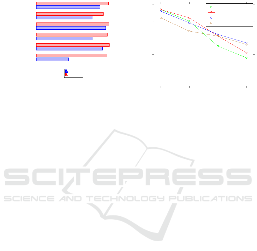
Unﬁltered

Filtered

Figure 5: The improvements in the neural network’s output

accuracies after applying ﬁltering to the training data. After

ﬁltering the problem is more learnable. The results were

measured during the training of the GRU model. Each row

shows the ﬁnal validation accuracy of the network’s outputs

at the end of training.

each program in the training process. In all of the ex-

periments, we created the test datasets by sampling

the original program space uniformly at random, with

a sample size of 1000.

4.1 Filtering the Datasets

Filtering the datasets using the method described in

Section 3.1 made the problem more learnable for

the neural network, resulting in improvements in the

case of each output head of the network. The exact

changes can be seen in Figure 5.

This ﬁltering is used on all datasets in all experi-

ments.

4.2 Different Recurrent Layers

In this section, we compare the effect of different re-

current layers on accuracy. We ran experiments with

LSTM (Hochreiter and Schmidhuber, 1997), bidirec-

tional LSTM (Schuster and Paliwal, 1997), GRU, and

bidirectional GRU.

In the ﬁrst experiment, we looked at the accuracy

of the different layers as the composition length in-

creased (Figure 6). The bidirectional layers proved to

be suboptimal, as these – somewhat surprisingly – did

not make the system more accurate for longer func-

tion compositions, but training and testing both took

considerably more time.

Despite the fact that bidirectional LSTM achieves

better accuracy for shorter compositions, its accuracy

falls below regular LSTM and GRU cells as the com-

position length increases. It is also the slowest of the

three in terms of execution time. The bidirectional

GRU model is the second slowest, and its accuracy is

the worst of the layers tested for longer compositions.

2 3 4

100

Composition length

Accuracy [%]

Bidirectional GRU

Bidirectional LSTM

GRU

LSTM

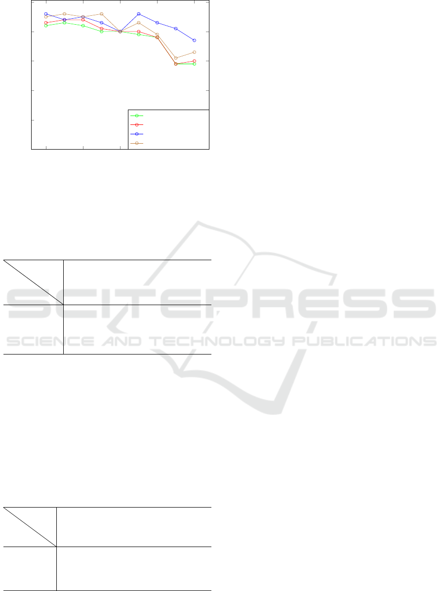
Figure 6: The performance of different recurrent layers in

relation to the number of functions used in the composi-

tion. In the case of both bidirectional models and the LSTM

model, we used a hidden state consisting of 200 neurons.

For the GRU model, we increased this amount to 256, as the

GRU cells require less computation. Although the bidirec-

tional LSTM performs the best with shorter compositions,

its performance decreases remarkably as the composition

length increases, and it is also the slowest. Considering

speed and accuracy the GRU model is the most favorable.

Between the regular LSTM and GRU cells, GRU is

preferred as it performs well in terms of both execu-

tion time and accuracy.

In the second experiment, we checked how Flex-

Coder scales based on the length of the input-output

examples in terms of accuracy. We generated prog-

ram input-output vectors with a length of 10 to 50

in increments of ﬁve for testing purposes. Figure 7

shows that FlexCoder with GRU was capable of gen-

eralizing well to longer inputs.

Similarly to the ﬁrst experiment, GRU was the

most accurate while being the best in terms of ex-

ecution time. Both bidirectional models performed

similarly, but the bidirectional LSTM was markedly

slower. The GRU model performed consistently bet-

ter than the LSTM-based network on longer example

lengths.

Based on the results of these two experiments, we

elected to use GRU as the recurrent layer of the archi-

tecture.

4.3 Accuracy and Execution Time

Tables 3 and 4 show the accuracy and the time needed

to ﬁnd a solution in terms of the number of input-

output pairs and the composition length. By increas-

ing the number of input-output pairs the problem be-

comes more speciﬁc: ﬁnding a program that ﬁts all

the pairs becomes a more complex task because the

ICPRAM 2021 - 10th International Conference on Pattern Recognition Applications and Methods

392

10 20 30 40

100

Length of input examples

Accuracy [%]

Bidirectional GRU

Bidirectional LSTM

GRU

LSTM

Figure 7: The accuracy of FlexCoder using four different re-

current layers as a function of the length of the input. GRU

generalizes best to longer input lengths.

Table 3: Relation between composition length, the number

of input-output pairs, and the accuracy. Increasing compo-

sition length or the number of pairs almost always decreases

the accuracy.

comp.

length

#I/O

pairs

1 2 3 4 5

2 97% 97% 97% 96% 97%

3 99% 94% 92% 95% 93%

4 97% 89% 86% 83% 85%

5 96% 88% 81% 79% 78%

set of possible solutions narrows. Similarly, as we in-

crease the composition length the space of possible

programs also increases.

The accuracy achieved by FlexCoder is compara-

ble to PCCoder with the time limit replaced by the

same iteration limit as in FlexCoder. In terms of exe-

cution time FlexCoder sometimes falls behind, but the

performance of the two systems is generally similar.

Table 4: Relation between composition length, the number

of input-output pairs, and the execution time in seconds. In-

creasing either composition length or the number of inputs

almost always also increases execution time.

comp.

length

#I/O

pairs

1 2 3 4 5

2 211s 255s 264s 277s 274s

3 524s 1082s 1239s 1141s 1291s

4 1224s 2900s 3250s 3923s 3620s

5 1520s 3445s 4986s 5537s 5530s

4.4 Comparison with PCCoder

We compare our system to PCCoder which has out-

performed DeepCoder by orders of magnitude (Zohar

and Wolf, 2018).

Our approach to program synthesis is quite dif-

ferent from the approach of PCCoder (see Sec-

tions 1 and 3.1). We synthesize a function compo-

sition, they synthesize a sequence of statements. The

expressiveness of the grammars is also different: On

the one hand, our grammar is missing some func-

tions like ZipWith or Scan1l. On the other hand,

our grammar is much more expressive in terms of pa-

rameter values.

Our grammar is capable of expressing 151 diffe-

rent functions, 130 of which can be anywhere in the

sequence and 21 can only appear as the outermost

function as these return a scalar value. The DSL used

by PCCoder can express 105 different functions. The

number of possible programs with a length of ﬁve is

about 43.13 million for FlexCoder and about 12.76

million for PCCoder, resulting in our program space

being 3.38 times larger when considering programs

with a length of ﬁve.

To make fair comparisons despite these differen-

ces, we run experiments where both systems run on

their own dataset, and we also compare them by run-

ning them on the dataset of the other system.

In the ﬁrst experiment, we examine what we con-

sider a crucial aspect of any program synthesis tool:

how well it generalizes with respect to the length of

the input-output lists. We trained both PCCoder and

FlexCoder on input-output vectors of length 15 to 20

with composition length 5. For PCCoder we set the

maximum vector length to 50. We tested the systems

on input-output vectors with a length of 10 to 50 in in-

crements of ﬁve, having 5 input-output examples per

program, each on their own dataset. The results can

be seen in Figure 8.

In the second experiment, we compare the accu-

racy of FlexCoder and PCCoder in a less realistic sce-

nario when PCCoder performs best: on the same in-

put lengths the systems have been trained on. In this

experiment, PCCoder does not have to generalize to

different input lengths. We compare the systems both

on their own dataset and on the datasets of each other

in Figure 9.

Our approach deﬁnes a depth limit for the search

algorithm, while the search used by PCCoder has a

time limit. To make the experiment fair, we changed

our algorithm’s depth limit to a time limit, and chose a

timeout of 60 seconds like PCCoder. The introduction

of a time limit in our search algorithm makes our sys-

tem’s accuracy go down by a couple of percent com-

Flexcoder: Practical Program Synthesis with Flexible Input Lengths and Expressive Lambda Functions

393

10 20 30 40

100

Length of input vectors

Accuracy [%]

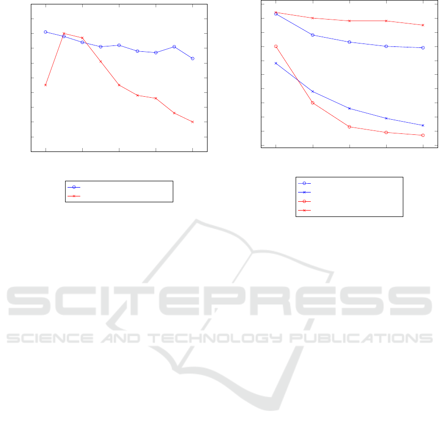
FlexCoder on FlexCoder data

PCCoder on PCCoder data

Figure 8: The accuracy of FlexCoder and PCCoder in rela-

tion to the length of the input. Both systems were trained

on input-output vectors of length 15 to 20 with composition

length 5. For PCCoder we set the maximum vector length

to 50. We tested the systems on input-output vectors with

a length of 10 to 50 in increments of ﬁve, having 5 input-

output examples per program, each on their own dataset.

pared to Figure 7, so FlexCoder could perform even

better with the original depth limit. The parameters

in this experiment are the same as in the ﬁrst exper-

iment, except for the length of the input lists which

is the same as for training, and the number of input-

output examples which range from 1 to 5.

5 DISCUSSION

FlexCoder generalized well with respect to the input

length in contrast to PCCoder. PCCoder only excelled

on vector lengths it was trained on. PCCoder has an

upper limit on the length of the input-output vectors;

we set the maximum vector length of PCCoder to 50

to accommodate this experiment. Applying PCCoder

to longer inputs would require retraining with a larger

maximum vector length.

We also compared the two systems when the in-

puts are the same length for testing as for training,

so PCCoder does not need the generalize to diffe-

rent input lengths. In this easier and less realistic

scenario, both systems beat the other on their own

dataset. Also, both systems perform notably worse

on the DSL of the other system.

We suspect that the reason behind the worse per-

formance of FlexCoder in this scenario is that in

these ﬁrst experiments, we used function composi-

1 2 3 4

100

Number of I/O pairs

Accuracy [%]

FlexCoder on FlexCoder data

PCCoder on FlexCoder data

FlexCoder on PCCoder data

PCCoder on PCCoder data

Figure 9: The accuracy of FlexCoder and PCCoder on their

own and the other’s dataset. The parameters are the same

as in the ﬁrst experiment, except that no generalization over

the input length is needed: the length of the input lists is

the same as for training. The number of input-output pairs

range from 1 to 5.

tions where – apart from the ﬁxed parameters – each

function had only a single list as input and output.

Relaxing this constraint would raise the expressive-

ness of FlexCoder to a much higher level, and could

allow FlexCoder to outperform PCCoder in most ex-

periments.

One strength of FlexCoder in contrast to PCCoder

is the separation of operators and operands in the

lambda functions. Currently only two higher-order

functions (map and ﬁlter) are using these lambda

functions. We expect that FlexCoder would perform

better relatively to PCCoder if we extended the gram-

mar with more higher-order functions.

6 CONCLUSION

The DSL of DeepCoder is limited in terms of expres-

sivity as stated by the authors themselves in their sem-

inal DeepCoder paper. The main motivation of our

paper is to extend it and move towards real-world app-

lications.

We presented FlexCoder, a program synthesis sys-

tem that generalizes well to different input lengths,

separates lambda operators from their parameters, and

increases the range of integers in the input-output

pairs.

ICPRAM 2021 - 10th International Conference on Pattern Recognition Applications and Methods

394

The main limitation and the most promising fu-

ture work seems to be allowing function compositions

where each function can take more than one non-ﬁxed

parameter. This would allow our grammar to exp-

ress ZipWith, Scan1l, and other interesting compo-

sitions, like the composition that takes the ﬁrst n ele-

ments of a list where n is the maximum element of the

list. This could be expressed as take(max(arr),arr),

if we allowed expressions as parameters.

Further experimenting with our neural network

might include using NTM cells (Graves et al., 2014)

instead of GRU cells, as NTM cells are shown to work

exceptionally well when learning simple algorithms,

such as sorting which is also present in our set of used

functions.

FlexCoder proved to be accurate and efﬁcient even

when generalizing to input vectors with a length of

50, with much wider parameter ranges than current

systems. We hope that it represents a step towards the

wide application of program synthesis in real-world

scenarios.

ACKNOWLEDGEMENTS

The authors would like to express their gratitude to

Zsolt Borsi, Tibor Gregorics and Ter

ez A. V

arkonyi

for their valuable guidance. The materials were

produced as part of EFOP-3.6.3-VEKOP-16-2017-

00001: Talent Management in Autonomous Vehicle

Control Technologies. The Project is supported by the

Hungarian Government and co-ﬁnanced by the Euro-

pean Social Fund.

REFERENCES

Balog, M., Gaunt, A. L., Brockschmidt, M., Nowozin, S.,

and Tarlow, D. (2016). Deepcoder: Learning to write

programs. arXiv preprint arXiv:1611.01989.

Bird, S., Klein, E., and Loper, E. (2009). Natural language

processing with Python: analyzing text with the natu-

ral language toolkit. ” O’Reilly Media, Inc.”.

Cho, K., Van Merri

enboer, B., Gulcehre, C., Bahdanau, D.,

Bougares, F., Schwenk, H., and Bengio, Y. (2014).

Learning phrase representations using rnn encoder-

decoder for statistical machine translation. arXiv

preprint arXiv:1406.1078.

Chomsky, N. and Sch

utzenberger, M. P. (1959). The al-

gebraic theory of context-free languages. In Studies

in Logic and the Foundations of Mathematics, vol-

ume 26, pages 118–161. Elsevier.

Feng, Y., Martins, R., Bastani, O., and Dillig, I. (2018).

Program synthesis using conﬂict-driven learning.

SIGPLAN Not., 53(4):420–435.

Graves, A., Wayne, G., and Danihelka, I. (2014). Neural

turing machines. arXiv preprint arXiv:1410.5401.

Gulwani, S. (2016). Programming by examples: App-

lications, algorithms, and ambiguity resolution. In

Olivetti, N. and Tiwari, A., editors, Automated Rea-

soning, pages 9–14, Cham. Springer International

Publishing.

Gulwani, S., Polozov, O., and Singh, R. (2017). Program

synthesis. Foundations and Trends

 in Programming

Languages, 4(1-2):1–119.

Hochreiter, S. and Schmidhuber, J. (1997). Long short-term

memory. Neural computation, 9(8):1735–1780.

Kalyan, A., Mohta, A., Polozov, O., Batra, D., Jain, P., and

Gulwani, S. (2018). Neural-guided deductive search

for real-time program synthesis from examples. arXiv

preprint arXiv:1804.01186.

Kingma, D. P. and Ba, J. (2014). Adam: A

method for stochastic optimization. arXiv preprint

arXiv:1412.6980.

Klambauer, G., Unterthiner, T., Mayr, A., and Hochre-

iter, S. (2017). Self-normalizing neural networks. In

Advances in neural information processing systems,

pages 971–980.

Lee, W., Heo, K., Alur, R., and Naik, M. (2018).

Accelerating search-based program synthesis using

learned probabilistic models. ACM SIGPLAN Notices,

53(4):436–449.

Manna, Z. and Waldinger, R. (1975). Knowledge and rea-

soning in program synthesis. Artiﬁcial intelligence,

6(2):175–208.

Parisotto, E., rahman Mohamed, A., Singh, R., Li, L., Zhou,

D., and Kohli, P. (2016). Neuro-symbolic program

synthesis.

Schuster, M. and Paliwal, K. K. (1997). Bidirectional re-

current neural networks. IEEE transactions on Signal

Processing, 45(11):2673–2681.

Shapiro, E. Y. (1982). Algorithmic program debugging.

acm distinguished dissertation.

Yin, P., Zhou, C., He, J., and Neubig, G. (2018). Struct-

vae: Tree-structured latent variable models for semi-

supervised semantic parsing.

Zhang, W. (2002). Search techniques. In Handbook of data

mining and knowledge discovery, pages 169–184.

Zohar, A. and Wolf, L. (2018). Automatic program syn-

thesis of long programs with a learned garbage col-

lector. In Advances in Neural Information Processing

Systems, pages 2094–2103.

Flexcoder: Practical Program Synthesis with Flexible Input Lengths and Expressive Lambda Functions

395