
Using Goal Directed Techniques for Journey Planning with Multi-criteria
Range Queries in Public Transit
Arthur Finkelstein
1
and Jean-Charles R
´
egin
2
1
Instant System, Garden Space B2, Rue Evariste Galois, 06410 Biot, France
2
Universit
´
e C
ˆ
ote d’Azur, I3S, CNRS, France
Keywords:
Public Transit Routing, Shortest Path, Pareto Optimization, Preprocessing.
Abstract:
One of the main problems for a realistic journey planning in public transit is the need to give the user multiple
qualitative choices. Usually, public transit journeys involve 4 main criteria: the departure time, the arrival time,
the number of transfers and the walking distance. The problem of computing Pareto sets with these criteria is
called the Pareto range query problem. This problem is complex and difficult to solve within the constraints of
the industrial world of smartphone applications, like a response time of the order of a second. In this paper, we
present the Goal Directed Connection Scan Algorithm (GDCSA), an algorithm that allows, for the first time,
to solve this problem with run times of less than 0.5 seconds on most European city or country-wide networks,
like Berlin or Switzerland. In addition, GDCSA satisfies other industrial needs: it is conceptually simple and
easy to implement. It partitions the graph in geographically small areas and precomputes some lower bounds
on the duration of a trip in order to select for each itinerary a sub-set of these areas to decrease the number of
scanned connections. Combining this sub-set and a journey planning using 4 criteria, the number of scanned
connections is lowered by a factor of up to 17 times compared to the best algorithms (CSA and RAPTOR), the
number of nodes opened during the search is lowered by a factor of up to 2.9 and the query times are lowered
by a factor of up to 9 on metropolitan networks. The integration of GDCSA in a smartphone app backend
server led to an improvement in results by a factor of 5.
1 INTRODUCTION
1.1 Problem Description
With the advent of smartphones, millions of passen-
gers use computer-based journey planning systems to
obtain public transport directions. Those directions
need to be given in a reasonable amount of time, usu-
ally in less than a second, and a user does not want
only the shortest path from A to B but may want a
journey with the lowest walking distance, the least
transfers, something in between or any number of
combinations of criteria. A journey planning system
cannot guess what a passenger wants specifically so it
has to give directions containing more than one jour-
ney. This can be done by computing Pareto sets with
multiple criteria (arrival time, departure time, walk
distance, number of transfers, accessibility, ...). A lot
of work exists on the shortest path problem in public
transit but few integrate the real needs of the users:
not only the earliest arrival journey but a Pareto opti-
mal set of journeys.
Multiple variants of the public transport routing
problem exist: the profile variant solves simultane-
ously the earliest arrival problem for all source times,
the range query variant solves simultaneously the ear-
liest arrival problem for journeys that are at most two
times as long as the fastest journey. For each of those
variants we can add a Pareto set to solve a multi-
criteria problem, leading to the Pareto profile variant
and the Pareto range query variant.
The Pareto range query variant, mainly the one
that involves 4 criteria (departure time, arrival time,
number of transfers and walked distance) has a prac-
tical relevance because travelers do not want to ar-
rive significantly later than the earliest arrival time
and may have specific preferences on the number of
transfers or the walk distance. The two criteria for the
range query are the arrival and the departure time. The
other criteria provide a wide array of choices for the
user, which allows users to find a suitable answer ac-
cording to their mobility or their aversion to changing
vehicles. Note that the price is not used as a criteria
because most users have a transit subscription either
Finkelstein, A. and Régin, J.
Using Goal Directed Techniques for Journey Planning with Multi-criteria Range Queries in Public Transit.
DOI: 10.5220/0010235303470357
In Proceedings of the 10th International Conference on Operations Research and Enterprise Systems (ICORES 2021), pages 347-357
ISBN: 978-989-758-485-5
Copyright
c
2021 by SCITEPRESS – Science and Technology Publications, Lda. All rights reserved
347

where the user lives or when visiting another city as a
tourist, and therefore do not care about the price.
To solve this kind of problem there are mainly
two types of methods. The first one proceeds by
pre-processing and pre-calculating many solutions for
multiple hours (for example at night) in order to be
able to respond quickly to users. The second calcu-
lates solutions on demand. We can also imagine com-
bining these two types of methods.
The major drawback of preprocessing methods is
that they cannot integrate seamlessly the modifica-
tions that may appear on a network and that inevitably
occur every day. On the other hand, on-demand cal-
culation methods (called search methods) do not have
this problem, but they are too slow at the moment to
be used into a modern journey planning system.
In this paper, we propose to speed-up the response
time by guiding a search method using goal directed
techniques and using a little preprocessing not af-
fected by real-world hazards.
1.2 Proposed Solution
Algorithms that yield fast query times for public tran-
sit routing in large metropolitan networks are numer-
ous, with extensions of Dijkstra’s algorithm (Disser
et al., 2008; M
¨
uller-Hannemann et al., 2007; Pyrga
et al., 2008), graph labeling algorithms (Delling et al.,
2015a; Wang et al., 2015), non graph based algo-
rithms like the Connection Scan Algorithm (CSA)
(Dibbelt et al., 2018) or RAPTOR (Delling et al.,
2015b), preprocessing heavy approaches with Trans-
fer Patterns (Bast et al., 2010; Bast and Storandt,
2014), or with a lighter preprocessing with Trip-
Based Public Transit Routing (Witt, 2015). There
are also extensions to these algorithms to allow
for shorter response times, Trip Based Routing is
made faster with the use of condensed search trees
(Witt, 2016), RAPTOR with the use of hyper graphs
(Delling et al., 2017), CSA with the use of overlay-
graphs (CSAccel) (Strasser and Wagner, 2014) and
Transfer Patterns by reducing the space and time con-
sumption of the preprocessing (Bast et al., 2016b).
Among search based methods the two main ones
are CSA and RAPTOR. CSA based algorithms are
simple, short, easy to implement and have good per-
formances which makes them often used in jour-
ney planning systems (e.g. Instant System on the
Paris metropolitan network, TrainLine on the Euro-
pean train network, ...). In addition, the PRVCSA, the
Pareto range variant of the CSA, seems to be one of
the faster algorithms to solve the Pareto range query
problem as mentioned in multiple well-known articles
(Bast et al., 2016a; Dibbelt et al., 2018). Therefore,
we focus our study on CSA based algorithms.
In CSA, the connections are treated one after the
other, without distinguishing if they are useful or
not for the journey, CSA trades relevance of infor-
mation with simplicity and speed. Adding criteria
to the CSA leads to a performance degradation be-
cause more complex data structures are needed and
with each added criterion the size of the Pareto set in-
creases which decreases even more the performance.
In practice, for a system to be considered interactive it
should respond in less than 1 second. Unfortunately,
the PRVCSA does not have this performance when
more than three criteria are involved.
One way to achieve such a goal for the PRVCSA
is to combine it with goal-directed techniques, that
is to ”guide” the search toward the target by avoid-
ing the scan of an element (a vertex for Dijkstra, a
connection for the CSA) that is not in the direction
of the target. Classic algorithms using goal-directed
techniques are the A* search (Hart et al., 1968) and
the ALT algorithm (Goldberg and Harrelson, 2005)
which have been successfully used on road networks.
The CSAccel algorithm (Strasser and Wagner, 2014)
can be seen as the first combination of goal directed
technique and CSA. It applies CSA on multi-level
overlay graphs to reduce the number of scanned con-
nections and in doing so lower the run time. The main
idea behind CSAccel is to avoid looking at rural buses
that are neither near the departure city nor the arrival
city, and only keep a subset of connections between
cities. This reduces the number of scanned connec-
tions and the run time as well. CSAccel uses ex-
tremely sound principles and has significant gains on
country-wide networks. Unfortunately, it does not im-
prove run time for large dense metropolitan networks.
It is also a complex algorithm to implement.
In this article, we present GDCSA, a novel ap-
proach that combines goal-directed techniques with
the PRVCSA to allow the use of more criteria. We
reuse the principles behind CSAccel but in an easier
and more pragmatic way. We roughly use the same
idea of partitioning the graph but we introduce addi-
tional lower and upper bounds, and remove the multi-
level part of the partitioning. The key idea is to par-
tition the graph in areas and only use the connections
of a sub-set of the areas when computing a journey,
thanks to lower and upper bounds on the duration
of the public transit journey. The lower bounds are
computed in a preprocessing step for each pair of ar-
eas while the upper bounds are computed during the
journey planning. Each area is opened or discarded
with a simple evaluation between the upper bound
and the sum of two lower bounds (from the start stop
to the candidate area and from the candidate area to
ICORES 2021 - 10th International Conference on Operations Research and Enterprise Systems
348

the arrival stop). Then we merge the connections of
the chosen areas and launch the PRVCSA on this re-
stricted set of connections.
Our experiments reveal that on a large and dense
metropolitan public transit networks, the GDCSA al-
lows a journey planning using 4 criteria (departure
time, arrival time, number of transfers and walked dis-
tance) with a run time 2.5 to 9 times faster than the
PRVCSA and 4.3 to 16 times faster than the Pareto
range query variant of the RAPTOR. Thus, the jour-
ney planning can be used in an interactive setting
to satisfy the client’s needs (i.e. on the passenger’s
smartphone) with run times of less than 0.5 second on
most of the compared networks.
1.3 Integrating a Solution in an
Industrial Setting
We can identify multiple problems when integrating
an algorithm in an industrial setting: the accuracy of
the data, the maintainability and adaptability of the
algorithm and the integration into an existing system.
The problem when using public transport journey
planning systems on metropolitan data is that the data
is never 100% accurate, we can have multiple prob-
lems, e.g. circular lines that are not declared as such,
lines that have not been updated with the new stops
and departure times and any number of other prob-
lems. As such an algorithm that is robust to inaccurate
data is essential.
With inaccurate data and real life usage, we have
a lot of bug fixing and in a small company like ours
with 30 employees, any one of the R&D engineers
should be able to debug the core of the journey plan-
ning because a debug task is assigned independently
of who wrote the code. This means that an algorithm
that is easy to code, understand and maintain is vital.
An easily adaptable algorithm is important be-
cause each client has different needs, depending on
the size of the public transport network, the wish of
the community and other factors. This leads to an al-
gorithm that has to be easily modifiable. For example
certain clients want specific modes at the top or the
bottom, to use gps coordinates instead of stops as de-
parture and arrival, to combine free floating bikes or
kick-scooters with public transport which means jour-
neys to or from other modes will have specific con-
straints.
A complete app containing other components,
such as ticketing, next departure times, favorite no-
tification, guiding, transport on demand and more, in-
volves more complex data structures than the ones de-
scribed in the literature. For example simple iden-
tifiers are used for benchmarking whereas they are
more complex in an app to be human readable. So ac-
cess times to the data structures are longer and there-
fore the run time is slower. We also have the prob-
lem of persistence and the need for databases which
limit access times, and when connecting to real time
providers the correspondence between the line and
stop ids is never automatic.
During the development of the GDCSA, we made
sure to integrate all those aspects and we will give ex-
perimental results as well as results of an integration
in an industrial backend server.
This paper is organized as follows: Section 2 will
give all the notions necessary to understand the algo-
rithm. Section 3 introduces the GDCSA, the intuition
behind it and how the transit network graph is par-
titioned. Section 4 presents the experimental evalu-
ation of the algorithm on the performance and other
metrics. Section 5 concludes with a summary and a
discussion of future work.
2 PRELIMINARIES
In this section we formalize the inputs and algorithms
used in this work, we use the same formalization as
the CSA (Dibbelt et al., 2018) because it is the cen-
terpiece of our algorithm.
2.1 Timetable
A timetable represents for one specific day the vehi-
cles that exist (train, bus, tram, ferry, ...), when they
travel, where they travel and how passengers can go
from one vehicle to another. A timetable is a quadru-
ple (S, T,C, F) of stops S, trips T , connections C and
footpaths F:
• A stop is a position outside of a vehicle where a
passenger can wait. At a stop (and only at a stop)
a vehicle can halt and passengers can leave or get
on.
• A trip is defined by a vehicle going through stops
at fixed times. Formally a trip is a scheduled ve-
hicle: a journey done by a unique vehicle from a
starting stop to a last stop at a fixed time and made
of connections.
• A connection is a vehicle going from one
stop to another with no intermediate stops, it
is a sub-part of a trip. It is a quintuple
(c
dep stop
, c
arr stop
, c
dep time
, c
arr time
, c
trip
) whose
attributes are the departure stop, the arrival stop,
the departure time, the arrival time and the trip
of c respectively. Each connection must respect
two conditions: c
dep stop
6= c
arr stop
and c
dep time
<
Using Goal Directed Techniques for Journey Planning with Multi-criteria Range Queries in Public Transit
349

c
arr time
. All the connections of a trip form
a set. This set can be ordered in a sequence
c
1
, c
2
, . . . , c
k
such that c
i
arr stop
= c
i+1
dep stop
and
c
i
arr time
< c
i+1
dep time
for all i.
• The footpaths are used to model transfers, in other
words how to get from one vehicle to another.
They are neither trips, nor connections. Formally
a footpath f is a triple ( f
dep stop
, f
arr stop
, f
dur
).
Going from a connection c to a connection c
0
with
c
trip
6= c
0
trip
is possible if and only if:
– A footpath from c
arr stop
to c
0
dep stop
exists
– c
0
dep time
− c
arr time
> f
dur
+ s
change
The inequality allows a passenger to be sure the
transfer can be done even if one or both of the ve-
hicles have a delay. The variable s
change
depends
on the departure stop, arrival stop and modes for
each of these stops. A loop is introduced on each
stop to allow a passenger to get off at a stop and
take another trip going through this stop.
Example. We will use the public transit network of
New York City.
Trips can be done by trains, trams, buses, ferry
and other modes of transportation that have fixed de-
parture and arrival times. Let t be a trip of the line 1
of the metro going to ”South Ferry” with a departure
date at 08/16/19 3:14 PM. The trip without a depar-
ture date is not a unique identifier because this trip
exists each day of the week.
If we take 3 consecutive stops of t ”50 Street”,
”Times Square - 42 Street” and ”34 Street - Penn Sta-
tion”, then there is a valid connection with ”50 Street”
as a departure stop, ”Times Square - 42 Street” as an
arrival stop and t as a trip. There is another valid con-
nection with ”Times Square - 42 Street” as a departure
stop, ”34 Street - Penn Station” as an arrival stop and
t as a trip. A non-valid connection is a connection that
has ”50 Street” as a departure stop, ”34 Street - Penn
Station” as an arrival stop and t as a trip because there
exists an intermediate stop (i.e. ”Times Square - 42
street”).
2.2 Journeys
A journey describes how a passenger can travel
through a public transit network. It is made of legs
that are pairs of connections (l
i
enter
, l
i
exit
) from the
same trip. l
i
enter
must appear before l
i
exit
in the trip
or l
i
enter
= l
i
exit
if the trip has only one connection.
Formally a journey is composed of legs and foot-
paths alternately f
0
, l
0
, f
1
, l
1
, . . . , f
k
, l
k
. A journey
must start and end with a footpath, which can be a
self loop.
2.3 Connection Scan Algorithm
Given a source stop s, a target stop t, a minimum de-
parture time τ and a timetable T , the CSA outputs a
journey with the minimum arrival time over all jour-
neys that depart after τ from s and arrive at t. This
earliest arrival variant assumes that the connections
are stored as a sorted array using the departure time of
the connections, and that the footpaths are stored in a
data structure that allows an iteration over the incom-
ing or outgoing footpaths. A connection is reachable
if a passenger can get on the connection. Similarly to
Dijkstra’s algorithm, tentative arrival times are stored
for each stop but a priority queue is not used. Instead,
the CSA iterates over all the connections (sorted by
departure time) and tests if they are reachable. For
each reachable connection, the algorithm updates the
tentative arrival time for each stop that can be reached
by foot from the arrival stop of the connection. The
CSA is significantly faster than Dijsktra’s algorithm
even though it touches more connections, because the
work required per connection does not involve a pri-
ority queue operation.
2.3.1 Variants of the Connection Scan Algorithm
The CSA can be extended to account for all of the
source times with the profile variant. This is still done
by scanning the ordered connections only once, but
the journeys are constructed from late to early and the
algorithm exploits the fact that an early journey can
only have later journeys as sub-journeys. We then can
add a Pareto set to solve a multi-criteria problem, the
Pareto profile variant. When adding one criterion, the
code can be modified in a specific way to avoid de-
creasing the performances too much but when adding
more the code needs to be generic leading to a bigger
decrease in performance.
Another way the CSA can be extended is the range
query variant, where we only solve the earliest arrival
problem for journeys that are at most two times as
long as the fastest journey, the solution to this problem
is a sub-set of the solution to the profile problem. In
the same way as before, we can also then add a Pareto
set to solve a multi-criteria problem, the Pareto range
query variant. This algorithm is the PRVCSA.
3 GOAL-DIRECTED
TECHNIQUES MEET CSA
From now on we will only consider the Pareto range
query variant of the journey planning in public transit
ICORES 2021 - 10th International Conference on Operations Research and Enterprise Systems
350

with the 4 criteria mentioned in the introduction (de-
parture time, arrival time, walking distance and num-
ber of transfers).
CSAccel (Dibbelt et al., 2018) uses goal-directed
techniques in the form of multi-level overlay graphs.
A multi-level (hierarchical) partition of the stop set
is done, this approach relies on small balanced graph
cuts and while they can easily be found between cities
on a country-wide scale, it is significantly more diffi-
cult to do so for a particular city. CSAccel works on
a hierarchical graph that is organized geographically,
large cells at the top and small cells at the bottom. A
level corresponds to a geographic abstraction of the
reality, the goal is to avoid scanning all the connec-
tions of a given cell. This is done with a preprocess-
ing step by keeping a sub-set of the connection in a
cell that will allow us to go through it, called transit
connections, because a core observation is that con-
nections in a journey where a passenger does not get
off or on a bus do not need to be scanned. This al-
lows the CSAccel to scan a lower number of connec-
tions by identifying potential relevant cells and only
using their transit connections. CSAccel is strongly
dependent on its non-obvious hierarchical graph par-
titioning and has a significant increase in code and
algorithmic complexity compared to CSA, as said by
its authors.
Our approach is simpler. It partitions the graph
in areas, on a single level, and uses lower and upper
bounds to open a sub-set of areas needed to compute
the journey that will lead to a smaller search space,
i.e. the number of connections, and in doing so the
run time is lowered as well.
The idea behind the algorithm is that when com-
puting a journey between New York and Washington,
it is important to look at trips going between the two
cities as well as those that go a little bit off-course,
i.e. Atlantic City. On the other hand looking at trips
near Boston or Syracuse will only lengthen the jour-
ney, thus we can safely remove those trips from the
search space.
3.1 Partitioning the Graph
Intuitively, we want to geographically partition the
timetable to allow a preprocessing step to compute
lower bounds to guide the search of the GDCSA.
In order to define the geographical partitioning,
we present some notations and define the core con-
cepts of: geographical graph of a timetable, areas,
boundaries and geographical partitioning.
3.1.1 Geographical Graph
A geographic graph G = (S, E) can be abstracted from
a timetable T where S is the set of stops, E is the set
of edges and M is the seconds of a day such that
(u, v) ∈ E ⇒ ∃t
1
,t
2
∈ M, z ∈ T | (u, v, t
1
,t
2
, z) ∈ C (1)
3.1.2 Area
An area a is a connected sub-graph of G. The ar-
eas partition the graph, i.e. they are pairwise disjoint,
such that the union of the parts give you the entire set
of stops.
We have a few definitions for an area:
• A connection c belongs to an area a if and only if
c
dep stop
∈ a.
• For all u ∈ S, A(u) is the area containing u.
• Let connections(a) be the list of connections of
the area a.
Figure 1: Example of an area.
3.1.3 Boundary of an Area
The boundary of an area a is the set of stops B(a) ⊆ a
who have at least one edge with an extremity outside
of the area a.
The boundary B(a) contains the stops that allow
us to leave an area a to reach another and to get to the
internal stops of other areas. They are the red stops in
the Figure 1.
3.2 Management of Candidate Areas
We have two definitions for the duration in public
transport:
• An upper bound of the duration in public transit
between two stops s and t ∈ S, with a departure
time τ
s
is written d
PT
(s,t, τ
s
).
• A lower bound of the duration in public transit
between two stops s and t ∈ S is written d
PT
(s,t).
Using Goal Directed Techniques for Journey Planning with Multi-criteria Range Queries in Public Transit
351
Goal directed techniques aim to guide the search to-
ward the target by avoiding the scan of unnecessary
stops. We apply the same techniques only to the areas
of the graph G to avoid scanning connections that will
only take us away from the target. By using upper and
lower bounds on the duration between stops and more
specifically between the areas.
Opening or not a candidate area will either add
the connections of an area to the search space of the
current journey computation if it is opened or discard
them if the candidate area is not opened.
Given s, t ∈ S. A candidate area a is opened when
computing a journey from s to t at time τ
s
if and only
if
d
PT
(A(s), a) + d
PT
(a, A(t)) ≤ d
PT
(s,t, τ
s
) (2)
Traversing an area cost 0 in time because the lower
bounds are always computed using stops on the
boundary.
s
t
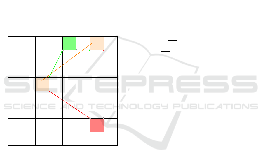
Figure 2: Example of an area opening.
The opening of an area is schematized in Figure 2,
let us assume the shortest path between points is the
length of a straight line. The green and red arrows
represent the lower bounds between the areas and the
orange arrow represents the upper bound between s
and t. Two areas are depicted, the one in green will
be opened because the sum of the length of the green
arrow from the area containing s to the green area and
the length of the green arrow from the green area to
the area containing t (traversing an area cost 0) is less
than the length of the arrow between s and t. However
the red area will not be opened because the sum of the
length of the red arrow from the area containing s to
the red area and the length of the red arrow from the
red area to the area containing t is greater than the
length of the arrow between s and t.
3.2.1 Upper Bound on the Duration
Intuitively, the upper bound on the duration is found
by quickly computing the size of the search span be-
cause a user isn’t interested in journeys that arrive sig-
nificantly later than the earliest arrival time.
We use the maximum arrival time τ
t
as defined in
(Dibbelt et al., 2018), which is equal to
τ
t
= τ
s
+ 2 · (x − τ
s
) (3)
Where x is the earliest arrival time. This upper bound
is advantageous because it is realistic e.g. consider
a traveler departing at 8:00 AM and arriving at the
earliest at 9:00 AM, then journeys arriving after 10:00
AM can be discarded because they are not of practical
relevance.
The upper bound on the duration we use is
d
PT
(s,t, τ
s
) = τ
t
− τ
s
(4)
That is the time span to satisfy a journey request. We
can estimate d
PT
(s,t, τ
s
) easily:
d
PT
(s,t, τ
s
) = τ
t
− τ
s
= τ
s
+ 2 · (x − τ
s
) − τ
s
= 2 · (x − τ
s
)
(5)
The only unknown is x which is the earliest arrival
time and can be computed with a CSA in an extremely
small amount of time.
3.2.2 Lower Bound on the Duration
Intuitively, the lower bound on the duration between
two stops s and t is the minimum duration over all
the journeys of the day going from the the boundary
of the area containing s to the boundary of the area
containing t.
The lower bounds associated with an area a
s
is
computed by launching a PCSA, the profile variant
of the CSA. The start stops are the boundary of the
area, as if we could reach all of them instantly. Then,
we iterate over every other area and take the minimum
duration to reach the boundary of the area a
t
from the
boundary of the area a
s
. Algorithm 1 is a possible
implementation of these computations.
The lower bounds can be computed once and for
all in a preprocessing step, note that this preprocess-
ing step can be parallelized, because each PCSA is
independent and we don’t access the same variables
in memory, meaning the preprocessing time can be
reduced. And also because the lower bound is valid
for an entire day because public transit vehicle can
only be delayed and cannot arrive earlier than the time
written in the schedules.
ICORES 2021 - 10th International Conference on Operations Research and Enterprise Systems
352

Algorithm 1: Lower bound algorithm in pseudo-code.
function LOWER BOUND(G)
dur ← [G.areas()][G.areas()]
Creation of a duration matrix
for all a
s
∈ G.areas() do
r ← PCSA(B (a
s
))
We compute a PCSA using the boundary
as starting points
for all a
t
∈ G.areas() do
min dur ← +∞
Minimum duration to reach a
t
from a
s
for all b ∈ B (a
t
) do
min dur ← min(min dur, r[b])
end for
dur[a
s
][a
t
] ← min dur
end for
end for
return dur
end function
3.3 GDCSA
GDCSA works in four phases, the first computes the
upper bound, the second iterates over each area to
only keep the ones that will be useful to the jour-
ney planning, the third will merge all the connec-
tions from the chosen areas and the last will launch
a PRVCSA using the sub-set of connections.
Algorithm 2: GDCSA algorithm in pseudo-code.
function GDCSA(G, s,t, τ
s
)
L
a
← empty list
ub ← d
PT
(s,t, τ
s
)
We iterate over all areas of the graph
for all a ∈ G.areas() do
if d
PT
(A(s), a) + d
PT
(a, A(t)) ≤ ub then
L
a
.insert(a)
end if
end for
L
c
← empty list
We iterate over all opened areas of the graph
for all a ∈ L
a
do
L
c
.insertAll(connections(a))
end for
L
c
← sort(L
c
)
We only use the connections of the opened ar-
eas
return PRVCSA(G, s, t, τ
s
, L
c
)
end function
The GDCSA is described in the algorithm 2. We can
see 4 phases: the first computes the upper bound (line
3), the second opens areas (from line 5 to line 9), the
third retrieves the connections and sorts them (from
line 12 to line 15) and the last launches a 4 crite-
ria Pareto range query variant of the CSA using only
the sorted connections of the opened areas (line 18).
The first two parts (opening the areas and getting their
connections) are easy to code and understand leading
to an easy code implementation. We only need to pre-
compute the lower bounds but we do so using a profile
variant of the CSA which is also fast and easy to code.
3.3.1 Optimizations
Using the Earliest Arrival CSA Instead of the
Lower Bound. Instead of using equation 2 to open
a candidate area, we can use
d
PT
(s, r, τ
s
) + d
PT
(r, A(t)) ≤ d
PT
(s,t, τ
s
) (6)
by replacing the lower bound between the start stop
and a candidate area with the earliest arrival time al-
ready computed by the CSA.
This will let us discard more candidate areas, al-
lowing us to have a more fine-grained management of
the candidate areas.
Optimizing the Opening Time. All the connec-
tions of an area are not relevant, because the further
away we are from the start of the journey s the lower
the number of reachable connection there is. There-
fore, for an area a the first connection that can be
scanned by the PRVCSA has
c
dep time
≥ τ
s
+ d
PT
(A(s), a) (7)
So we only keep connections that have a departure
time greater than the first reachable connection. For
example, consider a journey from New York to Wash-
ington with a departure time at 3:00 PM, then an area
near Washington only needs to scan connections with
a departure time greater than 5:30 PM because the
lower bound between New York and Washington is
2 hours and 30 minutes. This leads to a lower number
of scanned connections.
Optimizing the Closing Time. The same optimiza-
tion can be done but for the last reachable connection.
The last connection of an area a that can be scanned
by the PRVCSA must satisfy
c
dep
time
≤ τ
t
− d
PT
(a, A(t)) (8)
So we only keep connections that have a departure
time lower than the last reachable connection.
Using Goal Directed Techniques for Journey Planning with Multi-criteria Range Queries in Public Transit
353

Table 1: Instance size.
Network Stops Connections Lines Trips Footpaths
Paris 44534 3209401 1864 150963 502291
Berlin 28651 1379755 1296 63569 62456
Stockholm 14258 703326 664 34799 22138
Germany 74398 3601420 3599 168024 599284
Switzerland 29844 2599675 5645 248826 27202
Table 2: Details of the GDCSA and the variants of the CSA on metropolitan and country wide public transit networks.
# Scanned # Updated
Instance Algorithm Query (ms) connections stops # Labels
Paris PRVRAPTOR 15701 – – –
PRVCSA 7858 346376 18029 453452
GDCSA 2981 67293 10835 165529
Berlin PRVRAPTOR 1971 – – –
PRVCSA 1383 290444 13855 221128
GDCSA 338 46696 7027 67477
Stockholm PRVRAPTOR 1451 – – –
PRVCSA 847 137403 6298 98767
GDCSA 89 19175 3147 26727
Germany PRVRAPTOR 2312 – – –
PRVCSA 2587 273317 5499 143329
GDCSA 529 26535 3825 53407
Switzerland PRVRAPTOR 2364 – – –
PRVCSA 1289 824012 10011 132970
GDCSA 147 46005 3437 21597
3.3.2 Geographical Partitioning
The areas partition the graph. Thus, by geograph-
ically partitioning the graph, a passenger can go
through an area using only its connections.
We partition the graph using the inertial flow algo-
rithm (Schild and Sommer, 2015), a simple and effi-
cient algorithm that minimizes the boundary between
the areas. This is done by sorting the list of stops us-
ing either latitude or longitude or both, choosing a cer-
tain percentage (lower than 50%) of stops at the start
and end of the sorted list, which will be the sources
and the sinks respectively. Then a flow algorithm is
used, the min-cut gives the smallest boundary that di-
vides the stops into two new areas. These steps are
repeated for each new area, until a maximum depth or
a minimum size of the area is reached.
For example, when partitioning New York City
and New Jersey the algorithm will try to find the
smallest boundary which would be the extremities of
the bridges connecting New York City to the main-
land.
Once the graph is partitioned, we precompute the
lower bounds.
4 EXPERIMENTS
We evaluate the GDCSA and compare it to the 4 cri-
teria Pareto range query variant of the CSA. Apart
from measuring the run times, we also report the time
needed for the preprocessing as well as other metrics
related to the size of the search space (i.e. number
of scanned connections, number of stops with at least
one label). We also compare the run time of the GD-
CSA to the run time of the 4 criteria Pareto range
query variant of the RAPTOR.
Our test instance is based on the data of the public
transit network of 3 cities (Paris, Berlin and Stock-
holm) and 2 country wide train networks (Germany
and Switzerland), the data is openly available via a
GTFS feed (https://transitfeeds.com/) which has been
downloaded in October 2019. The details of the size
of the instances are in table 1.
ICORES 2021 - 10th International Conference on Operations Research and Enterprise Systems
354

Table 3: Performance of the precomputing on metropolitan public transit networks.
Paris Berlin Stockholm
Depth Query (ms) Prepro. (min) Query (ms) Prepro. (min) Query (ms) Prepro. (min)
8 3849 ∼ 33 450 ∼ 4 103 ∼ 2
9 3686 ∼ 39 408 ∼ 8 102 ∼ 3
10 3364 ∼ 61 379 ∼ 13 92 ∼ 5
11 3133 ∼ 96 357 ∼ 15 91 ∼ 8
12 2981 ∼ 172 338 ∼ 20 89 ∼ 12
13 2953 ∼ 315 323 ∼ 30 85 ∼ 14
14 2884 ∼ 413 317 ∼ 43 88 ∼ 16
Table 4: Performance of the precomputing on country-sized public transit networks.
Germany Switzerland
Depth Query (ms) Prepro. (min) Query (ms) Prepro. (min))
8 898 ∼ 26 238 ∼ 12
9 843 ∼ 43 217 ∼ 16
10 703 ∼ 73 195 ∼ 27
11 598 ∼ 120 187 ∼ 29
12 529 ∼ 178 147 ∼ 43
13 513 ∼ 240 132 ∼ 58
14 505 ∼ 301 129 ∼ 70
We can see that the city wide network range from
big with Paris, to smaller with Stockholm, the goal of
those metropolitan public transit network is to show
the performances of the GDCSA on dense networks.
Whereas the goal of the country wide train networks
is to show the performances on sparse networks.
The footpaths were given in the GTFS feed but the
graph was not transitively closed, we then program-
matically generated the missing ones.
We implemented all the algorithms in Java 8 and
run them with OpenJDK 8. All experiments were
conducted on a Intel Core i7-7700HQ processor with
16GiB of RAM.
In our evaluation, we ran for each variant of the
algorithm the same set of 1000 queries generated ran-
domly. The source and target stops are chosen uni-
formly at random. The departure time is picked uni-
formly at random within the day.
We ran a 4 criteria Pareto range query variant of
the CSA (PRVCSA in the table 2), as well as the
GDCSA, the 4 criteria are: maximizing the depar-
ture time, minimizing the arrival time, minimizing the
number of transfers and minimizing the walked dis-
tance. We also ran a Pareto range query variant of the
RAPTOR (PRVRAPTOR in the table 2) on the same
set of queries.
The GDCSA uses an Inertial Flow partitioning
with a maximum depth of 12.
The table 2 reports the average for the run time
(query), the number of scanned connections, the num-
ber of updated stops (stops that have at least one label)
and the total number of labels.
We can see that the run time of the GDCSA is 2.5
to 9 times faster than the PRVCSA. The run times for
the smaller networks have a greater gain from the GD-
CSA, whereas the bigger network the lower the gains
are. Across all the networks we see that the number
of updated stops (stops with at least one label), the
number of scanned connections and the number of la-
bels have considerably decreased when comparing the
PRVCSA and the GDCSA.
As for the results of the PRVRAPTOR, we can
see that the PRVCSA is 1.42 to 1.99 faster than
the PRVRAPTOR, except on the Germany network
where the PRVRAPTOR is faster due to the fact
that the number of journeys is extremely low. This
is in line with the results of (Bast et al., 2016a;
Dibbelt et al., 2018) where the same factors between
PRVRAPTOR and PRVCSA are shown.
Note that the gains from the GDCSA are really
good, one possible alternative would have been to
use the same ideas on the PRVRAPTOR. Unfortu-
nately there is no straightforward way to apply the
same ideas of partitioning the stops of the graph for
the PRVRAPTOR, as said in (Delling et al., 2017).
Using Goal Directed Techniques for Journey Planning with Multi-criteria Range Queries in Public Transit
355

4.1 Precomputing the Lower Bound
Precomputing the lower bound is done by launching
a profile variant of the CSA for each area.
We benchmark the partitioning and precomputing
on 5 public transit networks, with a maximum depth
for the Inertial Flow going from 8 to 14.
As we can see from table 3 and 4, the preprocess-
ing time is quite short. It takes on average 30 minutes
except for the biggest city-wide and country-wide net-
work where the preprocessing is close to 3 hours. All
those results are sequential, and the longest part of
the preprocessing can be easily parallelized (the pro-
file variant of the CSA for each area), meaning that a
large gain is possible.
For the query times, we can see that a query with
a maximum depth of 12 has the most gain compared
to the preprocessing time and that with a maximum
depth of 14 the gains are not worth the added prepro-
cessing time.
4.2 Integration in an Industrial Product
The GDCSA is integrated in an industrial backend
server for a smartphone app, with less than 1000
lines of code added. We achieve the same results as
those found for the European networks, on a large and
sparse instance of comparable size to the Germany in-
stance we see that the GDCSA is 5 times faster than
the PRVCSA. While also being a more complex prob-
lem, the departure and arrival stops can be GPS coor-
dinates, mixing multiple modes of transportation (car,
scooter, ...).
With a volume of only 1000 lines, this means that
an external engineer could comprehend the code and
then be able to modify it in less than a day.
5 CONCLUSION
In this article we presented an improvement of the
CSA to compute Pareto range queries by introduc-
ing additional upper and lower bounds that guide the
search by safely discarding areas that are not needed
during the search. The GDCSA uses preprocessed
lower bounds between each areas, and upper bounds
that are computed during the journey planning. It also
uses the PRVCSA as a center-piece which receives as
an input the sorted list of connections from the opened
areas. This leads to a simple implementation, with
an already working Pareto range query variant of the
CSA, the only code needed is the earliest arrival and
the profile variants of the CSA. Furthermore the algo-
rithm is easily extensible, because the addition or re-
moval of a criterion is made simple by the fact that the
upper and lower bound computation are not affected
by the Pareto criteria.
Our experiments on large realistic metropolitan
and country-wide public transit network have shown
that the GDCSA is up to 9 times faster than the
PRVCSA when computing 4 criteria Pareto range
queries. An interactive use can be considered for most
networks with a response time near or under 0,5 sec-
ond, even if the Paris network is still too slow some
headway has been made.
For future works, we would be interested in using
other graph partitioning. One other interesting direc-
tion to look in would be the addition of real time infor-
mation (delays, strikes, major events, ...) in the pub-
lic transit journey computation. And lastly, we could
look at the computation of the lower bounds and try
to make them closer to the optimal by adding a tem-
poral aspect with the computation of the lower bound
for every 4 hour span of a day.
ACKNOWLEDGEMENTS
This work has been supported by the 3IA C
ˆ
ote
d’Azur, Interdisciplinary Institute for Artificial Intel-
ligence (ANR-19-P3IA-0002) and by ANR project
MULTIMOD (ANR-17-CE22-0016).
REFERENCES
Bast, H., Carlsson, E., Eigenwillig, A., Geisberger, R., Har-
relson, C., Raychev, V., and Viger, F. (2010). Fast
routing in very large public transportation networks
using transfer patterns. In European Symposium on
Algorithms, pages 290–301. Springer.
Bast, H., Delling, D., Goldberg, A., M
¨
uller-Hannemann,
M., Pajor, T., Sanders, P., Wagner, D., and Wer-
neck, R. F. (2016a). Route planning in transporta-
tion networks. In Algorithm engineering, pages 19–
80. Springer.
Bast, H., Hertel, M., and Storandt, S. (2016b). Scalable
transfer patterns. In 2016 Proceedings of the Eigh-
teenth Workshop on Algorithm Engineering and Ex-
periments (ALENEX), pages 15–29. SIAM.
Bast, H. and Storandt, S. (2014). Frequency-based search
for public transit. In Proceedings of the 22nd ACM
SIGSPATIAL International Conference on Advances
in Geographic Information Systems, pages 13–22.
Delling, D., Dibbelt, J., Pajor, T., and Werneck, R. F.
(2015a). Public transit labeling. In International Sym-
posium on Experimental Algorithms, pages 273–285.
Springer.
Delling, D., Dibbelt, J., Pajor, T., and Z
¨
undorf, T. (2017).
Faster transit routing by hyper partitioning. In 17th
ICORES 2021 - 10th International Conference on Operations Research and Enterprise Systems
356

Workshop on Algorithmic Approaches for Transporta-
tion Modelling, Optimization, and Systems (ATMOS
2017). Schloss Dagstuhl-Leibniz-Zentrum fuer Infor-
matik.
Delling, D., Pajor, T., and Werneck, R. F. (2015b). Round-
based public transit routing. Transportation Science,
49(3):591–604.
Dibbelt, J., Pajor, T., Strasser, B., and Wagner, D. (2018).
Connection scan algorithm. Journal of Experimental
Algorithmics (JEA), 23:1–56.
Disser, Y., M
¨
uller-Hannemann, M., and Schnee, M. (2008).
Multi-criteria shortest paths in time-dependent train
networks. In International Workshop on Experimental
and Efficient Algorithms, pages 347–361. Springer.
Goldberg, A. V. and Harrelson, C. (2005). Computing the
shortest path: A search meets graph theory. In Pro-
ceedings of the sixteenth annual ACM-SIAM sympo-
sium on Discrete algorithms, pages 156–165. Society
for Industrial and Applied Mathematics.
Hart, P. E., Nilsson, N. J., and Raphael, B. (1968). A for-
mal basis for the heuristic determination of minimum
cost paths. IEEE transactions on Systems Science and
Cybernetics, 4(2):100–107.
M
¨
uller-Hannemann, M., Schulz, F., Wagner, D., and Zaro-
liagis, C. (2007). Timetable information: Models and
algorithms. In Algorithmic Methods for Railway Op-
timization, pages 67–90. Springer.
Pyrga, E., Schulz, F., Wagner, D., and Zaroliagis, C. (2008).
Efficient models for timetable information in public
transportation systems. Journal of Experimental Al-
gorithmics (JEA), 12:1–39.
Schild, A. and Sommer, C. (2015). On balanced separa-
tors in road networks. In International Symposium on
Experimental Algorithms, pages 286–297. Springer.
Strasser, B. and Wagner, D. (2014). Connection scan
accelerated. In 2014 Proceedings of the Sixteenth
Workshop on Algorithm Engineering and Experiments
(ALENEX), pages 125–137. SIAM.
Wang, S., Lin, W., Yang, Y., Xiao, X., and Zhou, S.
(2015). Efficient route planning on public transporta-
tion networks: A labelling approach. In Proceedings
of the 2015 ACM SIGMOD International Conference
on Management of Data, pages 967–982.
Witt, S. (2015). Trip-based public transit routing. In
Algorithms-ESA 2015, pages 1025–1036. Springer.
Witt, S. (2016). Trip-based public transit routing using con-
densed search trees. arXiv preprint arXiv:1607.01299.
Using Goal Directed Techniques for Journey Planning with Multi-criteria Range Queries in Public Transit
357
