Deep-Learning-based Segmentation of Organs-at-Risk in the Head

for MR-assisted Radiation Therapy Planning

László Ruskó

, Marta E. Capala

, Vanda Czipczer

, Bernadett Kolozsvári

, Borbála Deák-Karancsi

Renáta Czabány

, Bence Gyalai

, Tao Tan

, Zoltán Végváry

, Emőke Borzasi

, Zsófia Együd

Renáta Kószó

, Viktor Paczona

, Emese Fodor

, Chad Bobb

, Cristina Cozzini

, Sandeep Kaushik

Barbara Darázs

, Gerda M. Verduijn

, Rachel Pearson

, Ross Maxwell

Hazel Mccallum

Juan A. Hernandez Tamames

, Katalin Hideghéty

, Steven F. Petit

and Florian Wiesinger

GE Healthcare, Budapest, Hungary

GE Healthcare, Szeged, Hungary

Erasmus MC Cancer Institute, Department of Radiation Oncology, Rotterdam, The Netherlands

Erasmus MC, Department of Radiology and Nuclear Medicine, Rotterdam, The Netherlands

University of Szeged, Department of Oncotherapy, Szeged, Hungary

Newcastle University, Northern Institute for Cancer Research, Newcastle, U.K.

GE Healthcare, Munich, Germany

GE Healthcare, Milwaukee, U.S.A.

Keywords: Organ-at-Risk, Head, Radiation Therapy, MRI, Segmentation, Deep Learning, U-Net.

Abstract: Segmentation of organs-at-risk (OAR) in MR images has several clinical applications; including radiation

therapy (RT) planning. This paper presents a deep-learning-based method to segment 15 structures in the head

region. The proposed method first applies 2D U-Net models to each of the three planes (axial, coronal,

sagittal) to roughly segment the structure. Then, the results of the 2D models are combined into a fused

prediction to localize the 3D bounding box of the structure. Finally, a 3D U-Net is applied to the volume of

the bounding box to determine the precise contour of the structure. The model was trained on a public dataset

and evaluated on both public and private datasets that contain T2-weighted MR scans of the head-and-neck

region. For all cases the contour of each structure was defined by operators trained by expert clinical

delineators. The evaluation demonstrated that various structures can be accurately and efficiently localized

and segmented using the presented framework. The contours generated by the proposed method were also

qualitatively evaluated. The majority (92%) of the segmented OARs was rated as clinically useful for radiation

therapy.

1 INTRODUCTION

Head-and-neck cancers are one of the most common

cancers worldwide causing more than 200 000 deaths

per year (Tong et al., 2018). Radiation therapy (RT)

is an important treatment option for head-and-neck

cancer. In a state-of-the-art radiation therapy

treatment plan, radiation dose is shaped precisely to

the tumor. In that way, high energy photon/particle

beams can eradicate cancer cells while sparing as

much healthy tissues as possible. In the treatment

preparatory phase accurate definition of the target

volumes and organs-at-risk is essential. In the current

clinical practice, the planning phase of radiation

therapy is highly dependent on computer tomography

(CT) scans, hence it provides the electron density data

for the dose calculation algorithms. Therefore, it is

common practice that the structure contouring takes

place on the CT scans using information of further,

more sensitive imaging modalities either separately

or in fusion to the planning CT scans. Magnetic

resonance (MR) is becoming more and more

widespread as an additional imaging modality, due to

its high contrast for soft tissues, high spatial

resolution, non-ionizing radiation and non-invasive

nature. These properties render MR imaging superior

to the CT for cancer diagnosis and treatment

planning, as precise detection and localization of the

tumorous growth and surrounding organs-at-risk

Ruskó, L., Capala, M., Czipczer, V., Kolozsvári, B., Deák-Karancsi, B., Czabány, R., Gyalai, B., Tan, T., Végváry, Z., Borzasi, E., Együd, Z., Kószó, R., Paczona, V., Fodor, E., Bobb, C.,

Cozzini, C., Kaushik, S., Darázs, B., Verduijn, G., Pearson, R., Maxwell, R., Mccallum, H., Hernandez Tamames, J., Hideghéty, K., Petit, S. and Wiesinger, F.

Deep-Learning-based Segmentation of Organs-at-Risk in the Head for MR-assisted Radiation Therapy Planning.

DOI: 10.5220/0010235000310043

In Proceedings of the 14th International Joint Conference on Biomedical Engineering Systems and Technologies (BIOSTEC 2021) - Volume 2: BIOIMAGING, pages 31-43

ISBN: 978-989-758-490-9

(OARs) is crucial. For this reason, MR-only RT

planning solutions are under heavy research, where

the required electron density data is derived from a

pseudo-CT created from the MR scan (Wiesinger et

al., 2018). This workflow would be more convenient

for the patient, as one single MR examination would

deem enough for RT planning, as opposed to current

practice where the patient is scanned on different

imaging devices, often several times. Moreover, the

additional radiation dose from the CT scan could also

be avoided.

Currently, the standard clinical practice often

consists of manual contouring of OARs, which is

performed for various structures slice-by-slice by

experienced clinicians. This process is time

consuming (takes usually several hours per patient),

expensive and introduces inconsistencies due to both

intra- and inter-observer variabilities (Chlebus et al.,

2019). The unmet need for precise and automated

segmentation tools is unquestionable. Deep-learning-

based methods for image segmentation can bridge the

limitations of traditional atlas and machine learning

algorithms which are less suited to generalize for

unseen patient anatomies. Convolutional neural

networks (CNNs) are frequently used in medical

image analysis. In 2018, a model-based segmentation

method was proposed (Orasanu et al., 2018) applying

a CNN-based boundary detector to get better results

compared to the boundary detector using classic

gradient-based features. In the past few years U-Net

architectures (Ronneberger et al., 2015) became the

new state-of-the-art for image segmentation. For

example, a method proposed in (Mlynarski et al.,

2019) uses a 2D U-Net for multi-class segmentation

of 11 head organs and applies a graph-based

algorithm that forces the connectivity between

neighbouring organs. Both, Lei et al. (2020) and Chen

et al. (2019) developed a framework that first

localizes and then segments 8 and 6 head-and-neck

OARs, respectively. The method proposed in (Lei et

al., 2020) utilizes 3D Faster R-CNN to detect the

locations of OARs and uses attention U-Net to

segment them, while the algorithm in (Chen et al.,

2019) uses standard 3D U-Nets (Çiçek et al., 2016) in

a cascade manner in a way that it uses prior

segmentations (e.g. brainstem and eyes) to determine

the bounding box of the next target OAR (e.g. optic

nerves). Our proposed method utilizes a similar

approach, where the target OAR is first roughly

localized and then fine-segmented.

The presented method describes a U-Net deep

neural network architecture to segment various OARs

in the head region, crucial for radiotherapy planning.

As an initial step for head-and-neck OAR

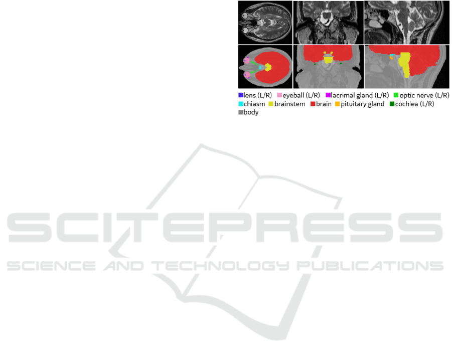
segmentation, we aim to segment a total of 15

relevant structures in this region, including structures

of the optic system (eyeballs, lenses, lacrimal glands,

optical nerves, chiasm), as well as the brain,

brainstem, pituitary gland, cochleas, and patient body

contour. Examples of these structures are shown in

Figure 1.

Figure 1: Manual annotations of organs-at-risk in head

region. Upper row: T2-weighted MR images in axial,

coronal and sagittal directions, respectively. Lower row:

manual annotations of the 15 organs-at-risk.

The difficulties in segmenting organs within the

head region, originates from suboptimal image

resolution and low contrast between neighbouring

tissues. For better segmentation, we developed a two-

stage framework for separately locating the target

OAR with 3 slice-based 2D models and segmenting it

with a 3D model. Additionally, for larger structures

(body, brain), which might not be completely covered

on the scan, only one 2D model is utilized for

segmentation.

The proposed method differs from the algorithm

in (Chen et al., 2019) as it is not a cascaded approach,

so the segmentation of OARs does not depend on the

segmentation of other OARs, similarly to the method

in (Lei et al., 2020). Additionally, different models

are trained independently for each organ unlike in

(Mlynarski et al., 2019). Another main difference

from the previously mentioned state-of-the-art

methods is that the proposed method is applied to

segment more OARs in the head region. Furthermore,

the models’ accuracy is also evaluated on an unseen

dataset with different MR image acquisition settings

from a separate source than the source of the training

dataset.

2 METHODS

The proposed method is based on deep learning

image segmentation. The algorithm starts with a

localization step that involves training 2D U-Net

BIOIMAGING 2021 - 8th International Conference on Bioimaging

models on axial, coronal and sagittal planes, fusing

their prediction maps, and using it to determine the

location of each organ by a surrounding 3D bounding

box. After this step, the proper image part with a

safety margin is cropped from the 3D image and a 3D

U-Net model is used to segment this smaller area.

This approach results in significantly less false

positive voxels in the segmentation and allows

considerably faster model training and inferencing.

This section describes the image datasets used in

this study, the model architecture, the details of the

model training, and the applied pre- and post-

processing methods.

2.1 Image Dataset

The image dataset incorporated in this work is a

combination of a publicly available dataset and a

private database. The public dataset is from the RT-

MAC (Radiation Therapy – MRI Auto-Contouring)

challenge hosted by the American Association of

Physicists in Medicine (AAPM), referred to as

AAPM dataset (Cardenas et al., 2019). The AAPM

dataset (available at The Cancer Imaging Archive

(TCIA) website (Clark et al., 2013)) includes 55 T2-

weighted images of the head-and-neck region with 2

mm slice thickness and 0.5 mm pixel spacing,

acquired with Siemens Magnetom Aera 1.5T scanner.

All scans have a matrix size of 512x512x120 points

and a squared 256 mm field of view. In most of the

scans, the top of the head is missing.

The private database (acquired by our clinical

partners) consists of 24 T2-weighted MR images

depicting the head-and-neck area, scanned using

different T2-weighted MR sequences (2D

PROPELLER, 2D FRFSE, 3D CUBE), with slice

thickness between 0.5 and 3 mm. These scans were

acquired on volunteers, using GE scanners

(MR750w, SIGNA (PET/MR, Artist, Architect)).

These scans, unlike the ones in the AAPM dataset, are

not uniform, and differ in MR image parameter

settings (e.g. resolution, pixel spacing). The models

in this study were trained solely on the publicly

available dataset and evaluated on both the public and

private databases.

Manual labelling for the AAPM dataset was done

by medical students under the supervision of a

medical doctor experienced in clinical delineation,

according to the RTOG and DAHANCA guidelines

(Brouwer et al., 2015). The list of structures was

defined together with radiation oncology specialists,

prioritizing those structures that are important for RT

planning of head-and-neck tumors. Irradiating these

structures above dose constraints would cause severe

side effects. For example if the anterior visual

pathways – optic nerves and chiasm – are exposed to

excessive radiation, it may lead to radiation-induced

optic neuropathy, which is defined as a sudden,

painless, irreversible visual loss in one or both eyes

occurring up to years after radiation treatment

(Akagunduz et al., 2017). Excessive radiation

exposure can be avoided by optimizing irradiation

parameters, like dose, beam shape and direction.

As not all scans included every organ (e.g. in

some scans only half of the eyeballs were present),

the number of manual segmentations varies for each

structure. The number of contours per structure can

be found in Table 1, where positive slices refer to the

(axial) slices in every MR image in the AAPM dataset

that contain the structure and negative slices are the

ones that does not contain the structure.

Table 1: Number of contours drawn in the AAPM datasets

and the count of positive and negative (axial) slices per

organ (left side/right side). (g.:gland).

Structure No. of

contours

Pos.

slices

Neg. slices

(

L/R

)

22/22 290/287 2350/2353

lens (L/R) 22/22 113/115 2527/2525

lacrimal

(

L/R

)

22/22 179/175 2461/2465

optic nerve (L/R) 36/36 158/162 4162/4158

chias

35 97 4103

rain 31 1244 2476

rainste

30 975 2625

ituitary g. 28 108 3252

cochlea

(

L/R

)

31/31 79/73 3641/3647

ody 29 3480 0

The contoured cases were separated into 3 subsets

(training, validation, and testing) using 60:20:20

ratio. The number of the training and validation

samples varied organ by organ, however, the test set

included the same 5 cases for all organs. The train-

validation- and test samples were used to optimize the

model, to select the best model, and to evaluate the

best model, respectively. For each organ the same

train/validation/test separation was used for both 2D

and 3D segmentation models.

From the private dataset (that was only used

during evaluation) 5 out of 24 scans were selected for

quantitative evaluation. The annotations for all 15

structures on these scans were defined by radiation

oncologists. In all of the private cases the

segmentation result was qualitatively evaluated. The

manual contour is referred to as gold standard in the

rest of the paper.

Deep-Learning-based Segmentation of Organs-at-Risk in the Head for MR-assisted Radiation Therapy Planning

2.2 Preprocessing

The following preprocessing was applied to the image

dataset before model training and inferencing. First,

the voxel size was normalized to be nearly equal to

1x1x1 mm (using integer factor for up or down-

sampling). Then, the images were cropped or padded

with zero voxels to have 256x256x256 resolution.

Finally, min-max normalization was applied to

intensity values, such that the intensity belonging to

99.9 histogram percentile was used instead of the

global intensity maximum.

Additional preprocessing was applied to the

image in case of body segmentation, which attempts

to eliminate background noise using multilevel

thresholding of Otsu’s method and morphological

operations (including closing, dilation, and removal

of air objects connected to the edge of the image).

2.2.1 Harmonization

The scans in the private database have different

intensity range compared to the AAPM dataset.

Therefore, an image harmonization step was

introduced prior to the data preprocessing, which

changes the intensity of the image to be statistically

similar to the reference image chosen from the

training samples.

For image harmonization, each MR volume 𝐼 was

decomposed into images belonging to different

energy band images:



𝐿



,𝑖1,…,B



using:

𝐿





𝑥



 𝐼



𝑥



, 𝐿





𝑥



 𝐿





𝑥



∗𝐺



𝑥;𝜎





(1)

where 𝐺 is a Gaussian kernel and 𝜎



is randomly

selected increasing number. Furthermore, let

𝐼





𝑥



 𝐿





𝑥



 𝐿





𝑥



𝑓

𝑜𝑟 i1,…,B1

(2)

𝐼





𝑥



 𝐿





𝑥



(3)

The above energy bands are computed for a reference

image (of the AAPM dataset). The aim is to make the

statistics (i.e. mean and standard deviation) of the

energy bands belonging to an input (𝑖𝑛) image similar

to that of the reference (𝑟𝑒𝑓) image:

𝐼









𝐼





𝑚𝑒𝑎𝑛



𝐼









∙

𝑠𝑡𝑑



𝐼







𝑠𝑡𝑑



𝐼







𝑚𝑒𝑎𝑛



𝐼







(4)

The harmonized image is computed by adding the

modified energy band images 𝐼





,𝑖1,…,B.

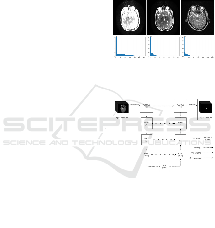
An example of the input, output and reference

image and their histograms is shown in Figure 2. The

motivation for this preprocessing step is to reduce

unwanted variability introduced by MR parameter

settings and to adjust the images of the private dataset

used for evaluation such as to be similar to the

training examples from the AAPM dataset. The

harmonization was only applied to the private dataset

before the evaluation.

Figure 2: Image harmonization. In the upper row, the input,

the harmonized and the reference image is shown,

respectively. The lower row shows their histograms in the

same order.

2.3 2D Model

Figure 3: Architecture of the 2D segmentation model used

for localization. The axial model is depicted on the figure,

but the same architecture is used for coronal and sagittal

models, as well.

The 2D model’s architecture (shown in Figure 3) is a

state-of-the-art U-Net, which is used to segment

structures on axial, coronal, or sagittal slices

independently (i.e. not using 3D information). The

size of the input is a 256x256 single-channel matrix

representing one slice of the MR image which

resolution is halved to 128x128 with a voxel size of

2x2x2 mm. The output is a 128x128 matrix with

prediction values, where 1 is the highest probability

indicating the presence of the organ, and 0 is the

lowest. The size of the output is increased to 256x256

using upsampling as the last layer.

BIOIMAGING 2021 - 8th International Conference on Bioimaging

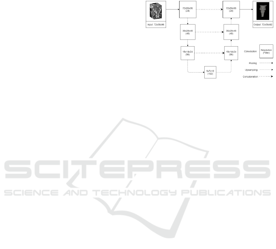
The model has 4 levels, at each level there are 2

consecutive convolution filters (with 3x3 kernel) with

batch normalization before the ReLU activation

layers. The number of filters is equal to 16 at the input

resolution and doubles after each pooling layer. The

model has 4 pooling layers (with 2x2 pool size), so

the resolution decreases to 8x8 (with 256 filters) at

the “bottom” of the network. Subsequently, the image

is gradually upsampled to the original resolution

using skip connections at each resolution level.

Each 2D model was trained for 75 epochs, except

the brain and body model, where the number of

epochs was set to 30. In each epoch 100% of positive

(including the organ) and the same number of

negative (not including the organ) slices were used.

Due to randomization, most of the negative slices are

used for training. For example, chiasm is detected in

97 positive slices (vide in Table 1), thus only 97 out

of 4103 negative slices are selected randomly in each

epoch. Note that less samples were used during

training than reported in Table 1, since that includes

all (train/validation/test) cases. This approach

accelerates and stabilizes the learning process and

increases the accuracy of the final model. Adam

optimizer was used with 8 batch size. The initial

learning rate was 0.001, and it was halved after every

25 epochs over the training process. During training,

accuracy and loss were calculated based on Dice. At

the end of each epoch the actual model was evaluated,

and the final model was selected based on the

validation loss.

Separate model was trained for each (axial,

coronal, sagittal) orientation. In case of paired organs,

both left and right structures were included in the

positive samples to increase the sagittal model’s

accuracy. For the two largest structures (brain and

body), which were partially covered in the input

images, only the 2D axial model was trained. In these

cases, the input resolution was equal to the original

512x512, the model architecture included 2 more (6

in total) pooling layers, and the model was trained for

30 epochs.

Although the accuracy of neither 2D model is

outstanding (except for the body and brain

segmentation), the combination of the 3 model

outputs is a good basis for the localization of the

organ. After applying each model (slice-by-slice) to a

3D volume, the 3 predictions are combined in the

following way. First, the predictions were binarized.

Then, those voxels were taken, where at least 2 of the

3 models predicted the organ. Finally, the largest

connected component was taken. This combination of

2D models is referred to as fused 2D model in the rest

of the paper.

2.4 3D Model with the Fused 2D

Localization

Figure 4: Architecture of the 3D segmentation model. The

input resolution varies by organ. The size of brainstem's

bounding box was used as an example.

The main advantage of the bounding box localization

for the 3D models is to speed up the training process

and increase the segmentation accuracy. The size of

the bounding box (encompasses the to-be-segmented

organ) was pre-defined and calculated based on the

whole training dataset. The centre of the bounding

box was computed from the gold standard during the

training, and it was computed from the fused 2D

model during the inferencing.

During the training of the 3D model, the bounding

box of the organ is cut from the preprocessed image

and fed into the CNN, thus the input of the network is

considerably smaller than the original resolution

(256x256x256). To account for possible inaccuracies

of the fused 2D model, the centre of the bounding box

was shifted with a random 3D vector before cutting

(using enough safety margin to include all voxels of

the organ) as an augmentation. In contrast to the 2D

model training, the histogram-based intensity

normalization as well as the additional mean/std

normalization was applied only to the bounding box

instead of the whole scan.

The architecture of the 3D model (shown in Figure

4) is created by changing the 2D model’s architecture

to accommodate the 3D input. The 2D layers are

replaced with 3D layers (convolution, pooling,

upsampling). The number of pooling layers is

decreased to 3 (using 2x2x2 pool size). The

convolutional layers use 3x3x3 kernel size. The

number of filters was increased to 24 at the input

resolution (and doubled after each pooling layer).

The 3D model was trained for 100 epochs. In each

epoch all training samples were used. The batch size

was reduced to 4 due to the increased memory needs

of the network. The same (Adam) optimizer and flat

(0.001) learning rate was used with best model

Deep-Learning-based Segmentation of Organs-at-Risk in the Head for MR-assisted Radiation Therapy Planning

selection based on validation loss. Training and

validation loss were defined with the Dice metric.

Separate 3D models were trained for each OAR.

During model inferencing the centre of bounding box

was calculated automatically (note that the size is an

organ specific constant) by taking the centre of the

bounding box of nonzero pixels in the result of the

fused 2D model.

2.5 Postprocessing

The prediction of the models was binarized using 0.5

threshold and resized to the original resolution.

Additional postprocessing was applied to body and

brain segmentations that involved filling the holes

and taking the largest connected component.

2.6 Evaluation

For each organ, all models (2D axial, 2D coronal, 2D

sagittal, fused 2D, 3D) were quantitatively evaluated

using the AAPM test set. Furthermore, the 3D models

were (qualitatively and quantitatively) evaluated on

the private cases. The following subsections describe

the evaluation methods.

2.6.1 Quantitative Evaluation

The segmentation results were compared with the

gold standard using Dice, and Surface Dice metrics.

The Dice similarity coefficient is the most

commonly used metric in validating medical image

segmentations by direct comparison between

automatic and manual segmentations. the formula for

calculating Dice is the following:

𝐷𝑖𝑐𝑒2 

𝑋∩𝑌

𝑋



𝑌

, (5)

where

𝑋

and

𝑌

are the number of voxels in the

automatic and manual segmentations, respectively

and

𝑋∩ 𝑌

is the number of overlapping voxels

between the two segmentations.

The limitation of this metric is that it weights all

inappropriately segmented voxels equally and

independently of their distance from the surface.

Thus, when comparing two segmentations, assessing

how well the surfaces of the contours are aligned can

provide useful information about the segmentation

accuracy. Surface Dice measures deviations in border

placement by computing the closest distances

between all surface points on one segmentation

relative to the surface points on the other (Wang et

al., 2019). The Surface Dice value represents the

percentage of surface points that lies within a defined

tolerance (as tolerance we used 1 and 2 mm).

To be able to compare the quantitative results to

the state-of-the-art, mean distance (MD) between

manual and automatic segmentation ( 𝑋 and 𝑌,

respectively) is defined as follow:

𝑀𝐷



𝑋,𝑌





𝑋



𝑌

 Inf

∈

𝑑



𝑥,𝑦



Inf

∈

𝑑



𝑦,𝑥



∈∈

 (6)

Where 𝑑 is Euclidean distance.

2.6.2 Qualitative Evaluation

The segmentations were qualitatively evaluated on

the private dataset by a radiation oncologist to assess

the usability of the segmented contours for

radiotherapy treatment planning (RTP). Each

segmentation result was classified into one of the

following 4 categories:

1. The contour is missing, or it can be used for

RTP after major corrections that would take

similar time as re-contouring.

2. The contour can be used for RTP after some

corrections that would take less time than re-

contouring.

3. The contour can be used for RTP after minor

corrections that would take significantly less

time than re-contouring.

4. The contour can be used for RTP without any

corrections.

2.7 Implementation Details

The deep learning training and inferencing

frameworks were implemented using Keras 2.3 with

Tensorflow 2.1 backend in Python 3.6 platform. The

2D and 3D models were trained and tested on an HP

Z440 workstation with 32 GB RAM, 12 core, 3.6

GHz CPU and GTX 1080, 8 GB RAM, 2560 CUDA

cores GPU.

3 RESULTS

3.1 Evaluation on AAPM Dataset

Figure 5 demonstrates the best and the worst 3D

results for all anatomy structures from the 5 test cases

of AAPM dataset. In the images the gold standard is

represented with red overlay, while the model

prediction is shown with green outline. All results are

displayed in the axial views.

BIOIMAGING 2021 - 8th International Conference on Bioimaging

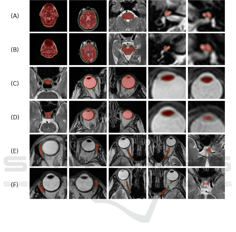
Figure 5: The best ((A), (C) and (E)) and worst ((B), (D) and (F)) segmentation results in the axial direction for the 15 OARs

((A) and (B) shows body, brain, brainstem, right and left cochlea, (c) and (D) shows the pituitary gland, right and left eyeball,

right and left lens, (E) and (F) shows right and left lacrimal gland, right and left optic nerve and chiasm). The predicted result

is depicted in green, and the gold standard is shown as a red overlay.

Table 2

demonstrates the Dice metric reflecting the

overall accuracy of the models and the Surface Dice

metric, which provides the surface accuracy within a

tolerated distance. The paired organs were trained and

tested separately (left and right part) except for the 2D

sagittal model, where both left and right parts were

used since location information is not included in

sagittal images (note that different accuracy of the left

and right sagittal models is due to randomization

during model training). According to the 2D results

the accuracy of the models is similar, and none of

them is significantly better than the other. It is

remarkable that the fused 2D model outperforms most

of the 2D models. The 3D model has an overall

outstanding performance compared to the other

models, except for the chiasm and the cochlea (R)

structures where the 3D model was only the second

best based on Dice accuracy.

3.2 Evaluation on Private Dataset

3.2.1 Qualitative Evaluation on the Private

Database

The proposed method was qualitatively evaluated on

the set of 24 T2-weighted MR images of the private

database for the 15 OAR structures. The results are

summarized in

Table 3

. Our models were able to

provide useful contour (i.e. rating ≥ 2) for 92% of the

segmentation tasks, and only 8% of the contours was

useless (including a few failed segmentations

indicated as bold numbers in the table).

Deep-Learning-based Segmentation of Organs-at-Risk in the Head for MR-assisted Radiation Therapy Planning

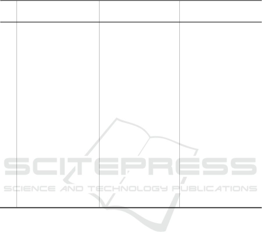
Table 2: 2D (axial (ax.), coronal (cor.), sagittal (sag.)), Fused 2D (F. 2D) and 3D model accuracy for 5 test cases of the public

dataset. (BS: brainstem, co.: cochlea, lac.:lacrimal gland, ON: optic nerve, pituit.:pituitary gland).

Dice (%) Surface Dice (%) (1 mm) Surface Dice (%) (2 mm)

ax.

cor.

sag.

F. 2D 3D

ax.

cor.

sag.

ax.

cor.

sag.

body 99.4 - - - - 98.1 - - - - 99.4 - - - -

brain 97.8 - - - - 94.5 - - - - 97.5 - - - -

BS 89.9 89.8 88.8 90.9 92.1 90.8 88.5 88.4 91.7 97.0 96.5 95.3 95.0 97.0 97.8

chiasm 63.5 56.9 54.3 62.6 59.2 86.0 81.8 84.9 87.5 91.9 89.3 87.6 89.8 91.9 93.5

co. (L) 62.8 65.7 67.5 72.9 82.3 90.7 85.8 86.1 94.9 97.3 95.0 88.8 89.0 97.3 100.0

co. (R) 61.9 60.7 63.1 76.2 72.1 95.1 74.1 80.4 98.0 99.9 98.9 76.3 82.7 99.9 99.8

eye (L) 92.6 89.1 93.7 93.7 93.9 98.9 92.0 98.0 98.7 99.7 99.7 97.0 99.3 99.7 100.0

eye (R) 92.3 93.7 93.5 94.2 94.6 96.8 98.3 98.0 99.2 99.9 98.5 99.8 99.0 99.9 100.0

lac. (L) 56.4 50.8 43.1 53.8 59.9 77.1 68.1 60.0 70.8 83.8 89.4 83.4 73.6 83.8 91.7

lac. (R) 44.8 49.5 49.1 50.3 57.5 70.5 66.7 64.7 71.0 83.9 84.2 79.9 75.5 83.9 88.7

lens (L) 74.2 75.5 74.5 77.7 79.7 93.6 96.3 98.0 98.3 99.4 97.3 98.1 99.7 99.4 99.9

lens (R) 75.6 73.6 75.0 76.9 81.5 96.1 95.0 97.5 97.3 99.5 99.0 97.6 99.3 99.5 99.7

ON (L) 68.1 61.3 66.0 71.6 73.7 88.4 82.0 87.9 89.8 93.9 93.4 88.1 93.0 93.9 95.8

ON (R) 65.7 63.9 65.5 69.3 71.5 88.7 84.7 87.2 89.1 92.5 93.7 90.0 91.7 92.5 95.7

pituit. 59.4 63.0 67.8 69.2 73.2 75.4 85.0 87.2 87.8 93.7 87.8 91.3 93.0 93.7 94.9

3.2.2 Quantitative Evaluation on the Private

Database

The models were also evaluated quantitatively on 5

annotated MR scans from the private database. The

summarized results of the 3D models are found in

Table 4 and Table 5. Compared to the results on the

AAPM test examples, the accuracy metrics are

somewhat lower. The models were able to provide

contour for all organs on each scan, except for Exam

14, where the proposed method for left lens failed and

segmented the right lens (more details in discussion).

3.3 Training and Segmentation

Efficiency

In this study, the training of a 2D model took 10-20

minutes (per image orientation) except for body and

brain, where it took several hours. The training of the

3D model took ~10 minutes per organ. Note that

during training no online augmentation was applied

to the images in addition to the random shift of the

bounding box. The average segmentation time (using

GPU) including the preprocessing, inferencing of

three 2D models, the computation of the bounding

box, and the inferencing of the 3D model, and the

post-processing took 30 seconds per organ per case.

4 DISCUSSION

Based on the quantitative evaluation metrics in Table

and Table 4, the average Dice score of the 3D and

2D axial models (for body and brain segmentation)

indicates that the proposed method was able to

segment the large anatomical structures with higher

than 90% Dice score on the AAPM dataset. However,

Dice metric was generally considerably lower for

BIOIMAGING 2021 - 8th International Conference on Bioimaging

Table 3: Qualitative evaluation of the private database by a radiation oncologist (MFS: Magnetic Field Strength, BS:

brainstem, pituit.: pituitary gland, cochl.: cochlea, ON: optic nerve, lacr.:lacrimal gland, PROP: Axial Propeller sequence) –

Bold numbers indicate the cases where the proposed method failed to segment the given organ. The exams that were used for

quantitative evaluation are highlighted in bold.

Sequence

(MFS)

body brain BS pituit.

cochl.

left

cochl.

right

chiasm

left

right

eye

left

eye

right

lacr.

left

lacr.

right

lens

left

lens

right

Mean

Exam 1 PROP (1.5T) 4 3 3 3 3 3 2 3 2 4 4 4 4 4 4 3.3

Exam 2 PROP (1.5T) 4 3 3 2 3 3 2 2 2 4 4 4 3 4 4 3.1

Exam 3 PROP (1.5T) 2 2 3 3 3 4 3 1 1 3 3 3 1 4 4 2.7

Exam 4 PROP (1.5T) 2 3 3 3 3 3 2 1 1 3 3 4 4 1 1 2.5

Exam 5 PROP (1.5T) 4 2 3 2 4 4 1 1 1 4 4 4 4 3 4 3.0

Exam 6 PROP (1.5T) 2 2 3 2 3 3 2 3 2 4 4 3 3 1 4 2.7

Exam 7 CUBE (3T) 2 1 2 1 3 3 2 2 2 3 3 3 3 4 3 2.5

Exam 8 CUBE (1.5T) 3 2 3 3 3 3 2 1 1 4 3 4 4 3 3 2.8

Exam 9

CUBE (3T) 4 2 3 2 3 3 2 2 2 3 3 3 4 3 2 2.7

FRFSE (3T) 3 3 3 2 2 2 3 2 2 3 3 3 3 3 3 2.7

Exam 10

PROP (3T) 4 2 3 2 4 4 2 3 3 3 3 3 1 4 4 3.0

FRFSE (3T) 3 2 4 2 3 3 2 3 3 3 3 3 4 4 3 3.0

Exam 11

CUBE (1.5T) 3 3 2 3 3 3 1 1 1 4 4 3 3 3 3 2.7

PROP (1.5T) 4 2 4 2 3 3 2 2 2 3 3 3 3 3 3 2.8

Exam 12

CUBE (1.5T) 3 2 3 3 2 3 2 2 2 3 4 4 4 3 3 2.9

PROP (1.5T) 4 2 3 3 4 4 2 3 4 3 4 3 4 3 4 3.3

Exam 13

CUBE (3T) 3 2 3 2 3 3 2 2 2 3 4 4 4 3 4 2.9

PROP (3T) 4 2 3 3 2 4 3 2 2 3 3 3 3 3 3 2.9

FRFSE (3T) 3 3 3 3 3 4 2 3 2 3 3 3 4 3 4 3.1

Exam 14

CUBE (1.5T) 2 2 3 2 3 3 2 1 2 3 3 3 3 1 3 2.4

PROP (1.5T) 4 3 4 1 3 3 3 2 3 4 3 3 3 1 4 2.9

Exam 15 CUBE (1.5T) 3 2 3 2 3 3 2 1 1 3 3 1 1 3 3 2.3

Exam 16

PROP (3T) 4 2 3 2 3 3 2 2 2 3 3 3 4 4 4 2.9

FRFSE (3T) 3 1 3 3 3 3 2 2 2 3 3 4 4 3 2 2.7

Mean 3.2 2.2 3.0 2.3 3.0 3.2 2.1 2.0 2.0 3.3 3.3 3.3 3.3 3.0 3.3

small structures (50-90%), where a slight mismatch

(that might be clinically irrelevant in terms of their

effect on radiotherapy treatment) can decrease the

accuracy significantly. The average Surface Dice in

Table 2 shows that at least 90% of segmented

structures’ surface was properly outlined within a

defined tolerance of 2 mm, meaning that only a small

fraction (maximum of 10%) of the surface needed to

be corrected compared to the gold standard surface.

These results indicate that the proposed method can

accurately segment various structures in the head

region.

Based on the qualitative evaluation on the private

dataset in

Table 3, the proposed method failed only on

small organs, such as pituitary gland (1), optic nerves

(3), lacrimal glands (3) and lenses (4). The reason

behind this might be that their 2D models (trained on

low number of positive slices) could not generalize

well. Therefore, there was no overlap between any

two of the 2D results when taking the majority vote.

This resulted in an empty fused 2D result, and as a

consequence, the bounding box for the 3D

inferencing couldn’t be generated. This can be

Deep-Learning-based Segmentation of Organs-at-Risk in the Head for MR-assisted Radiation Therapy Planning

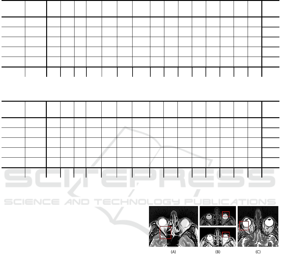
Table 4: Dice accuracy for 5 annotated case of private database. (BS: brainstem, pituit.: pituitary gland, cochl.: cochlea, ON:

optic nerve, lacr.:lacrimal gland).

Protocol body brain BS pituit.

cochl.

left

cochl.

right

chiasm

left

right

eye

left

eye

right

lacr.

left

lacr.

right

lens

left

lens

right

Mean

Exam 1 PROP 99.1 90.7 90.5 42.0 77.8 77.3 24.4 71.8 54.4 91.1 90.7 37.6 61.1 79.6 82.6 71.4

Exam 2 PROP 97.5 92.2 89.7 57.4 49.0 57.3 69.1 41.2 42.3 93.1 90.7 37.0 56.9 51.8 49.4 65.0

Exam 13 PROP 98.5 90.4 90.2 61.3 55.3 75.8 59.1 5.3 35.0 86.3 88.8 67.2 68.3 63.0 55.6 66.7

Exam 14 PROP 99.2 89.4 87.2 1.3 54.0 59.2 34.7 15.1 47.4 91.7 90.7 38.4 28.7 0.0 53.4 52.7

Exam 16 PROP 98.2 90.3 90.3 60.8 64.3 79.7 71.7 7.4 47.2 90.1 87.5 47.0 59.4 75.5 48.3 67.8

Mean 98.5 90.6 89.6 44.6 60.1 69.8 51.8 28.2 45.2 90.5 89.7 45.4 54.9 54.0 57.9

Table 5: Surface Dice (2 mm) accuracy for 5 annotated case of private database. (BS: brainstem, pituit.: pituitary gland,

cochl.: cochlea, ON: optic nerve, lacr.:lacrimal gland).

Protocol body brain BS pituit.

cochl.

left

cochl.

right

chiasm

left

right

eye

left

eye

right

lacr.

left

lacr.

right

lens

left

lens

right

Mean

Exam 1 PROP 99.4 81.4 91.4 96.0 95.1 99.6 92.2 95.2 84.9 100.0 99.1 79.5 95.5 98.9 99.2 93.8

Exam 2 PROP 98.6 81.4 96.4 96.5 79.6 86.5 96.1 75.0 91.9 99.9 99.2 76.0 88.5 90.0 87.7 89.6

Exam 13 PROP 98.6 77.5 96.0 92.5 97.4 91.0 81.6 22.6 72.0 99.1 99.5 90.9 88.1 92.1 86.2 85.7

Exam 14 PROP 99.0 75.2 87.9 20.5 97.0 99.1 84.5 49.4 88.7 99.4 98.5 84.0 80.4 0.0 86.9 76.7

Exam 16 PROP 96.7 89.3 96.6 92.0 93.9 98.1 96.3 27.0 82.0 99.3 99.2 73.6 94.1 98.7 94.2 88.7

Mean 98.5 81.0 93.7 79.5 92.6 94.9 90.2 53.8 83.9 99.5 99.1 80.8 89.3 76.0 90.8

later fixed by detecting these small structures in

connection with a larger organ located nearby.

In some cases, the failed results were due to image

properties that differed greatly from the training

dataset. In case of the optic nerve segmentation, in

two exams the low image quality resulted in poor

visibility of optic nerves that would also have

hampered the manual segmentation. An example is

shown in Figure 6.(A). In exam 14, the left lens

segmentation has failed since the structure was hardly

visible in the preprocessed image (shown in Figure

6.(B) lower image). The left lens was barely

observable in the original MR image (shown in

Figure 6.(B) upper image), which might have caused

its disappearance after preprocessing. Figure 7. shows

a case, where the right lens was segmented instead of

the left one. In this case the coronal model predicted

only false positive voxels within the right lens and the

sagittal model correctly segmented the right lens (as

it learns on both, left and right structure), so the 2D

model fusion involved the poorly segmented right

lens voxels, thus the bounding box was cut on the

wrong side. The lacrimal glands are usually

distinguishable from the eye, but in two cases the

lacrimal gland has disappeared into the surrounding

tissue, which led to the unsuccessful segmentation

(shown in Figure 6.(C)).

Figure 6: Examples for failed segmentation. (A) shows the

optic nerve which the model failed to segment. (B) depicts

the (upper) original and (lower) preprocessed MR image,

where the left lens disappears after preprocessing. (C)

represents the lacrimal gland which is barely

distinguishable from the neighbouring tissues.

The qualitative evaluation shows that 92% of the

models’ results achieved 2 or above qualitative score,

which means most of these segmentations were

clinically useful and only 8% of the segmentations

were classified into the first category which implies

that they can’t be utilized for radiotherapy planning.

BIOIMAGING 2021 - 8th International Conference on Bioimaging

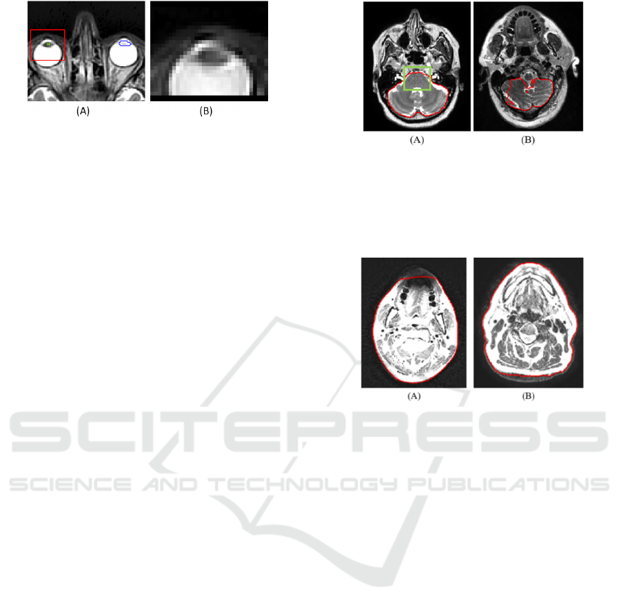
Figure 7: Faulty left lens segmentation. (A) Blue outline is

the gold standard; green outline marks the fused 2D result.

The red rectangle is the bounding box that is cut from the

image. (B) The bounding box of the left lens encompasses

the right lens due to the poor fused 2D result.

It is important to mention that the brain model was

trained on images where the top of the head was

missing (unlike most of the private cases), thus it was

not capable of properly segmenting the brain above

the ventricles. The qualitative evaluation did not,

while the quantitative evaluation did take this area

into account. Therefore, the average Dice score of the

brain model decreased compared to the result on the

AAPM test set significantly (from 97.8 to 90.6). The

2D brain model got an average of 2.2 qualitative

score, which means that most of the time it is still

useful for the radiotherapy planning, since the

correction of the results would require less time than

recontouring the whole organ. In the majority of the

results, that were rated as 2, the brain model failed to

differentiate between brainstem and brain tissues

resulting in over-segmentation. This might be caused

by the lack of spatial information due to only using a

2D model or due to the similar intensity of the upper

slices of brainstem and the white matter (shown in

Figure 8.(A)). Additionally, it was observed that in

certain cases the caudal part of the brain was under-

segmented. An example is presented in Figure 8.(B).

Although the 2D body model achieved relatively

high mean qualitative (3.3 out of 4) and quantitative

(Dice: 98.5) score on the private dataset, the radiation

oncologist noticed some typical faults in the

segmentation results during evaluation. Firstly, due to

some artefacts, the mouth area appeared as blurred in

the original MR image, and thus this part of the body

was under-segmented (represented in Figure 9.(A)).

The second observation was that, occasionally, the

caudal and in few cases, the cranial parts of the

contour were incomplete. An example of the under-

segmentation of the caudal part is depicted in Figure

9.(B).These two might be the results of the additional

preprocessing step for the body segmentation.

However, if we omit this step from the segmentation

process, large over-segmentation could occur around

the body due to background noise.

Figure 8: Segmentation faults of the brain model. Red

contour shows the brain segmentation. (A) depicts that the

brainstem (inside the green bounding box) is hardly

distinguishable from the white matter. (B) represents the

under-segmentation that occurred on the caudal part of the

brain.

Figure 9: Segmentation faults of body model. Red contour

shows the body segmentation. The images depict the under-

segmentation of (A) mouth and (B) caudal part. The image

intensity was changed to highlight the under-segmented

parts that fade into the background.

Out of the results of the 3D models, the pituitary

gland, optic nerves and chiasm got the lowest scores

during both the qualitative and quantitative

evaluation. These organs are the most difficult to

segment as they are small structures, only appearing

in 2-5 slices and their visibility is dependent on MR

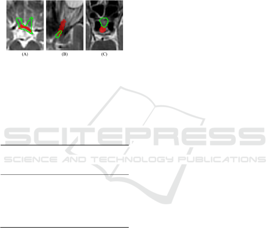
image parameter settings. In case of chiasm, if the

image has been acquired with an appropriate angle, it

is visible in 1-3 slices as an X-shaped structure,

slightly darker than its neighbouring tissues.

However, if the angle is different, the chiasm

becomes too fragmented, and hard to distinguish from

the surrounding brain matter. An example of an over-

segmented chiasm is shown in Figure 10.(A). With

regard to the optic nerves, in some cases they were

not clearly defined, and hard to distinguish from the

surrounding tissue. Such small structures are hard to

segment on scans with relatively large slice

thicknesses (3 mm or above), like the ones in the

private dataset. Consequently, this structure is

typically under-segmented (Figure 10.(B)).

Additionally, optic nerves can be hard to segment,

since they might consist of separate disconnected

Deep-Learning-based Segmentation of Organs-at-Risk in the Head for MR-assisted Radiation Therapy Planning

components on the image slices, as a result of the

slight curvature of the organ. The pituitary gland is

usually easy to contour, since it is a little orb situated

under the chiasmatic cross. However, the pituitary

gland is often inhomogeneous, thus the results can be

under-segmented. A poorly detected pituitary gland is

depicted in Figure 10.(C).

Figure 10: Examples of segmentation faults of the proposed

method that achieved the lowest Dice scores. Gold standard

is shown as red overlay, the prediction of the 3D model is

marked with green outline (A) depicts an over-segmented

chiasm. (B) shows an example of an under-segmented optic

nerve. (C) The 3D model was unable to localize the

pituitary gland inside the bounding box.

Table 6: Comparison of state-of-the-art Dice (%) and mean

distance (MD) (mm) results. (BS: brainstem, ONC: optic

nerves and chiasm, pitu.: pituitary gland). Under proposed

method, the metrics calculated for the AAPM test set are

shown.

Orasanu

et al.

(2018)

Mlynarski et al.

(2019)

Chen

et al.

(2019)

Proposed

method

MD Dice MD Dice Dice MD

brain

96.8 0.08

97.8 0.78

BS 0.56 88.6 0.26 90.6 92.1 0.62

ONC 0.80 67.4 0.48 75.7 65.9 0.61

eye 0.53 89.6 0.11 94.2 94.3 0.28

lens 0.67 0.63 58.8 80.6 0.22

pitu. 58.0 0.69 73.2 0.43

To the best of our knowledge, there are only three

prior publications on deep-learning-based OAR

segmentation of the head from MR images ( (Orasanu

et al., 2018), (Mlynarski et al., 2019) and (Chen et al.,

2019)) that reported Dice and/or mean distance (MD)

results (Mlynarski et al., 2019). To be able to compare

the results, the paired organs’ and optic nerves’ and

chiasm’s quantitative results were averaged and an

additional metric, the mean distance results were

calculated. Based on Table 6, the proposed method

outperforms the state-of-the art Dice scores for most

structures, while our mean distance results are

comparable to the state-of-the-art. However, the

comparison is difficult due to different datasets.

Orasanu et al. validated their results on 16 T2-

weighted MR images using 5-fold cross-validation,

Mlynarski et al. reported cross-validated results on a

dataset including 44 contrast-enhanced T1-weighted

MR images, Chen et al. used a dataset of 80 T1-

weighted MR images from which 20 was used during

testing, while in this work, a maximum of 26 T2-

weighted image were available for training.

The advantages of the proposed approach over the

standard 2D or 3D UNET solutions are the robust

localization that is based on more 2D models, and the

precise 3D segmentation that is efficient to train and

infer due to the reduced 3D domain. The

disadvantages are the need for maintaining more

models and the limited capability of segmenting

organs which are partially covered in the image.

5 CONCLUSION

In this paper, the segmentation of 15 head structures

was presented using the well-known deep-learning

architectures. Separate 2D models were trained to

segment various structures on axial, coronal, and

sagittal slices of MR images. For the body and brain,

a 2D axial model alone could provide accurate 3D

segmentation. For the other (smaller) organs, the

combination of the 2D models was used for accurate

localization of the organ’s bounding box that was

accurately segmented with a 3D model.

The proposed models were trained on a public

dataset and evaluated on both public and private

image database. Based on the quantitative results, the

presented approach was able to provide precise

segmentation of various structures in the head region

despite the limited size of the training database

(maximum of 26 data from the AAPM dataset) and

different challenges introduced by the private

database (in particular, different MR parameter

settings such as larger slice thickness, no head

fixation as in the AAPM dataset thus more artifact is

present). The qualitative evaluation given by a

radiation oncologist on the set of 24 MR images of

the private dataset demonstrated that the majority

(92%) of the segmentations were found clinically

useful for radiation therapy treatment planning. It also

showed that the proposed method was not sensitive to

different T2 sequences, which indicates its ability to

generalize. The presented approach demonstrates

competitive performance compared to the prior state-

of-the art in terms of Dice scores and mean distance.

In the future, we aim to improve organ models to

segment structures more accurately by increasing the

BIOIMAGING 2021 - 8th International Conference on Bioimaging

training dataset and utilizing more augmentations

during training. Furthermore, to decrease the

inferencing time, we intend to develop a multiclass

segmentation method based on the proposed

approach, which can also improve the robustness of

the localization. Finally, the presented approach can

be extended to other organs in the neck region.

ACKNOWLEDGEMENT

This research is part of the Deep MR-only Radiation

Therapy activity (project numbers: 19037, 20648)

that has received funding from EIT Health. EIT

Health is supported by the European Institute of

Innovation and Technology (EIT), a body of the

European Union receives support from the European

Union´s Horizon 2020 Research and innovation

programme.

REFERENCES

Akagunduz, O. O., Yilmaz, S. G., Yalman, D., Yuce, B.,

Biler, E. D., Afrashi, F., and Esassolak, M. (2017).

Evaluation of the Radiation Dose–Volume Effects of

Optic Nerves and Chiasm by Psychophysical,

Electrophysiologic Tests, and Optical Coherence

Tomography in Nasopharyngeal Carcinoma.

Technology in cancer research & treatment 16.6

(2017), 16(6), 969-977.

Brouwer, C. L., Steenbakkers, R. J., Bourhis, J., Budach,

W., Grau, C., Grégoire, V., . . . Langendijk, J. A. (2015).

CT-based delineation of organs at risk in the head and

neck region: DAHANCA, EORTC, GORTEC,

HKNPCSG, NCIC CTG, NCRI, NRG Oncology and

TROG consensus guidelines. Radiotherapy and

Oncology, 117(1), 83-90.

Cardenas, C. E., Mohamed, A. S., Sharp, G., Gooding, M.,

Veeraraghavan, H., and Yang, J. (2019). Data from

AAPM RT-MAC Grand Challenge 2019. The Cancer

Imaging Archive.

doi:https://doi.org/10.7937/tcia.2019.bcfjqfqb

Chen, H., Lu, W., Chen, M., Zhou, L., Timmerman, R., Tu,

D., . . . Gu, X. (2019). A recursive ensemble organ

segmentation (REOS) framework: application in brain

radiotherapy. Physics in Medicine & Biology, 2, 64.

Chlebus, G., Meine, H., Thoduka, S., Abolmaali, N., van

Ginneken, B., Hahn, H. K., and Schenk, A. (2019).

Reducing inter-observer variability and interaction time

of MR liver volumetry by combining automatic CNN-

based liver segmentation and manual corrections. PloS

one, 14(5), e0217228.

Çiçek, Ö., Abdulkadir, A., Lienkamp, S. S., Brox, T., and

Ronneberger, O. (2016). 3D U-Net: learning dense

volumetric segmentation from sparse annotation.

International conference on medical image computing

and computer-assisted intervention, 424-432.

Clark, K., Vendt, B., Smith, K., Freymann, J., Kirby, J.,

Koppel, P., Prior, F. (2013). The Cancer Imaging

Archive (TCIA): Maintaining and Operating a Public

Information Repository, Journal of Digital Imaging.

Journal of digital imaging, 26(6), 1045-1057.

https://doi.org/10.1007/s10278-013-9622-7.

Lei, Y., Zhou, J., Dong, X., Wang, T., Mao, H., McDonald,

M., Yang, X. (2020). Multi-organ segmentation in head

and neck MRI using U-Faster-RCNN. In Medical

Imaging 2020: Image Processing. International Society

for Optics and Photonics.

Mlynarski, P., Delingette, H., Alghamdi, H., Bondiau, P.-

Y., and Ayache, N. (2019). Anatomically Consistent

Segmentation of Organs at Risk in MRI with

Convolutional Neural Networks. arXiv preprint

arXiv:1907.02003.

Orasanu, E., Brosch, T., Glide-Hurst, C., and Renisch, S.

(2018). Organ-at-risk segmentation in brain MRI using

model-based segmentation: benefits of deep learning-

based boundary detectors. International Workshop on

Shape in Medical Imaging, Springer(Cham), 291-299.

Ronneberger, O., Fischer, P., and Brox, T. (2015). U-net:

Convolutional networks for biomedical image

segmentation. International Conference on Medical

image computing and computer-assisted intervention.

Tong, N., Gou, S., Yang, S., Ruan, D., and Sheng, K.

(2018). Fully automatic multi-organ segmentation for

head and neck cancerradiotherapy using shape

representation model constrained fullyconvolutional

neural networks. Medical physics, 45(10), 4558-4567.

Wang, Y., Zhao, L., Wang, M., and Song, Z. (2019). Organ

at risk segmentation in head and neck ct images using a

two-stage segmentation framework based on 3D U-Net.

IEEE Access 7

, 144591-144602.

Wiesinger, F., Bylund, M., Yang, J., Kaushik, S.,

Shanbhag, D., Ahn, S., Cozzini, C. (2018). Zero TE-

based pseudo-CT image conversion in the head and its

application in PET/MR attenuation correction and MR-

guided radiation therapy planning. Magnetic

Resonance in Medicine, 80(4), 1440-1451.

Deep-Learning-based Segmentation of Organs-at-Risk in the Head for MR-assisted Radiation Therapy Planning