
Two Stage Anomaly Detection for Network Intrusion Detection
Helmut Neuschmied
1
, Martin Winter
1
, Katharina Hofer-Schmitz
1
, Branka Stojanovic
1
and Ulrike Kleb
2
1
DIGITAL – Institute for Information and Communication Technologies, Joanneum Research GesmbH, Graz, Austria
2
POLICIES – Institute for Economic and Innovation Research, Joanneum Research GesmbH, Graz, Austria
Keywords:
Autoencoder, Deep Learning, Anomaly Detection, Network Intrusion Detection, Variational Autoencoder.
Abstract:
Network intrusion detection is one of the most import tasks in today’s cyber-security defence applications. In
the field of unsupervised learning methods, variants of variational autoencoders promise good results. The fact
that these methods are very computationally time-consuming is hardly considered in the literature. Therefore,
we propose a new two-stage approach combining a fast preprocessing or filtering method with a variational
autoencoder using reconstruction probability. We investigate several types of anomaly detection methods
mainly based on autoencoders to select a pre-filtering method and to evaluate the performance of our concept
on two well established datasets.
1 INTRODUCTION
The increase in number of cyber-attack tools and ex-
ploitation techniques makes any existing classical se-
curity defence mechanism not adequate enough. Ev-
ery day, new variants of malware with new signatures
and behaviours close to the expected user and system
behaviour (referred as ”normal”) appear. Especially
attacks lasting over a longer period of time and occur-
ring in several, unknown specificities - also termed
as Advanced Persistent Threads (APTs) - let security
defenders struggle in securing every endpoint and link
within their networked system in time. APTs are usu-
ally set as multi-stage attacks, where the initial (net-
work) intrusion step is often missed, leaving the sys-
tem open to later stages including extensive data exfil-
tration. Detection of early stages is very important in
order to get attention on a potentially ongoing attack,
and in order to avoid leak of confidential information
to the outside world, financial losses, or, even worse,
severe damage and fatalities (Alshamrani et al., 2019;
Stojanovi
´
c et al., 2020).
In recent years, much research has been conducted
on the automatic, robust detection of network intru-
sions at a very early stage (Ring et al., 2019; Pawlicki
et al., 2020). Due to the unknown structure of intru-
sions and continuously varying appearance and sig-
nature of descriptive features, unsupervised anomaly
detection methods became the only feasible method
dealing with the lack of training examples for that
class of attacks. This is because of the fact, that unsu-
pervised learning techniques do not need any labelled
training data for (unknown) anomaly classes.
Although various traditional unsupervised tech-
niques show promising result on anomaly detec-
tion during the last decades, especially deep-learning
based approaches gained much interest by the re-
search community. Various unsupervised neural-
network based techniques - mainly autoencoder ap-
proaches - have been investigated in literature. From
our literature research we found that variational au-
toencoders using reconstruction probability are the
most promising approach in terms of detection qual-
ity, especially for unsupervised learning tasks. Nev-
ertheless we identified that a substantial disadvantage
of these methods is the considerably higher comput-
ing time. This is hardly considered in the literature,
but it is an essential point for the practical appli-
cability for the huge amount of network data to be
processed. Therefore we identify the need for effi-
cient pre-filtering as an important step to overcome
the aforementioned shortcoming.
This paper proposes a two-stage anomaly detec-
tion approach for network intrusion detection. Be-
sides justification of the considerations made above,
in this paper we also present a novel two-stage ap-
proach using the concept of pre-filtering. We in-
vestigate several types of anomaly detection methods
mainly based on autoencoders to select a pre-filtering
method and to evaluate the improvements of this con-
450
Neuschmied, H., Winter, M., Hofer-Schmitz, K., Stojanovic, B. and Kleb, U.
Two Stage Anomaly Detection for Network Intrusion Detection.
DOI: 10.5220/0010233404500457
In Proceedings of the 7th International Conference on Information Systems Security and Privacy (ICISSP 2021), pages 450-457
ISBN: 978-989-758-491-6
Copyright
c
2021 by SCITEPRESS – Science and Technology Publications, Lda. All rights reserved

cept. For the evaluations we use the network intrusion
datasets CICID2017 (Sharafaldin et al., 2018), con-
taining recent data, and NSL-KDD (Tavallaee et al.,
2009), as mostly cited in literature.
2 RELATED WORK
Anomaly detection is a research field utilized in many
application areas such as Video-Processing (Ravi Ki-
ran and Parakkal, 2018), Network Monitoring and In-
trusion Detection (Kwon et al., 2017; Hodo et al.,
2017; Javaid et al., 2016), Cyber-Physical Systems
(Schneider and B
¨
ottinger, 2018) or monitoring in-
dustrial control systems (Y
¨
uksel et al., 2016). Re-
cently, the scientific community focused on using
anomaly detection methods for cyber-security ap-
plications (Duessel et al., 2017; Fraley and Can-
nady, 2017; Tuor et al., 2017; Xin et al., 2018),
and especially for intrusion detection as primary part
for the discovery of Advanced Persistent Threads
(APTs)(Alshamrani et al., 2019; Ghafir et al., 2018).
Chandola (Chandola et al., 2009) proposed a one-
class support vector machine (OCSVM) for anomaly
detection. This method is used to learn the region
boundaries in the multidimensional data space that
contains only the training data instances. A distance
function is then applied on testing-samples, report-
ing only values above a certain threshold as potential
anomaly candidates.
Inspired by recent success of deep-learning based
methods, especially so called autoencoder based ap-
proaches gained much interest by the research com-
munity (Schneider and B
¨
ottinger, 2018). In principle,
they are a special type of multi-layer neural networks
performing hierarchical and nonlinear dimensionality
reduction of the data, and they can work in an unsu-
pervised manner. Given a large amount of (normal)
data, they can be trained to reconstruct the input-data
as closely as possible by minimizing the reconstruc-
tion error on the network’s output. In their easiest
form, they typically consist of three, fully connected
parts, namely an input (encoder) and an intermediate
(hidden) layer with a lower number of nodes, and out-
put layer (decoder). The only way to reconstruct the
input properly is to learn weights so that the interme-
diate outputs of the nodes in the middle layers repre-
sent a limited but meaningful representation. Those
reduced representation in the so called bottleneck-
layer make the autoencoders predestined for outlier
or anomaly detection (Chen et al., 2017), because in
contrast to normal data reconstructed very well, the
reconstruction error of anomaly data the autoencoder
has not encountered before, will be high.
Probabilistic variational autoencoders (VAE-
Prob) proposed by An and Cho (An and Cho, 2015)
use the reconstruction probability to calculate a
probabilistic measure for the reconstruction of the
input data. This measure accounts not only the dif-
ference between the reconstruction and the original
input, but also the variability of the reconstruction by
considering the variance parameter of the distribution
function. Thus variables with large variance would
tolerate large differences in the reconstruction for
normal behaviour and no weighting of the reconstruc-
tion error with respect to the variability of individual
values of the input data vector is necessary. Another
major advantage is that a relative (percentage)
threshold value is used for anomaly detection and no
absolute threshold value has to be defined.
3 TWO-STAGE APPROACH FOR
ANOMALY DETECTION
Figure 1: Two-Stage anomaly detection: The first autoen-
coder filters the data to such an extent that the variational
autoencoder using reconstruction probability is able to eval-
uate this data in time (the feature vector z, the mean m and
the variance vector σ represent the bottleneck-layers).
In our research on the qualitative performance of vari-
ous methods for anomaly detection (see section 4) we
found the variational autoencoder using reconstruc-
tion probability to be the most promising approach.
Good detection results have been achieved, the vari-
ability of anomalies and normal data is properly mod-
elled and the detection threshold can be set relatively.
Since the decoder for one input feature vector must
be activated very often by the statistical evaluation the
method is relatively computationally expensive. Thus
we have the need for a pre-filtering method speed-
ing up the entire process for application to real world
problems.
Hence we propose to use a two-stage approach as
sketched in Figure 1. In the first step – referred as
pre-processing or filtering step – a fast anomaly de-
Two Stage Anomaly Detection for Network Intrusion Detection
451

tector filters out data which, with a very high prob-
ability, do not belong to any anomaly. The remain-
ing data are then evaluated by a second, more specific
anomaly detector providing more accurate decision.
For the first step we expect that a fast, multi-layer au-
toencoder can be used and trained specifically for this
task. But also classical machine learning approaches
for one-class problems (e.g. One-Class SVMs) could
be used. For the second step we propose to use of
VAE-Prob, not only because of the better qualitative
performance (see section 4), but also because of the
advantage of avoiding the definition of an absolute
threshold value for pre-processing. Instead we can
use an adaptive threshold value which is controlled
in such a way, that the VAE-Prob receives as much
data for analysis as can be processed with the given
computing capacities. This system thus adapts to the
amount of data to be analysed. The Input Data Buffer
is required for the time synchronization of the two
processing stages and provides feature sets for a de-
tailed analysis in the second stage if not filtered out.
4 IMPLEMENTATION AND
EVALUATION
As a first step, we evaluate several anomaly detec-
tion methods in order to check our assumptions made
in section 3, to select the most suitable method for
pre-filtering the data, and to verify that the VAE-Prob
delivers good results on its own (but also in a two-
step approach by comparison with other methods).
This evaluation is performed using the network intru-
sion datasets NSL-KDD and CICID2017. The first
one has been extensively used in literature for method
comparison purposes. The latter contains also com-
plete flow data and thus shows enhanced feasibility
for practical application.
In order to estimate how well unsupervised learn-
ing methods performs in comparison to supervised
learning, we tested one method which uses anomaly
data also for training. However, this method is not
considered for the two-stage approach. Please note,
that in the given implementation data that originates
from legitimate, benign sources is referred as ”nor-
mal” or ”benign” data, while data that originates from
malicious sources (cyber-attacks) is referred as ”mali-
cious” or ”anomalous” data. The implementation and
evaluation has been done in Python using Keras and
Tensorflow. For the training task we use several Win-
dows and Linux machines with diverse graphic cards
(GTX 1070, Quadro RTX 4000 and a TITAN X). The
evaluation of all implemented methods took place on
a Windows 10 machine (Intel Core i7-8700, 3.2 GHz)
Table 1: Parameter used for model optimization.
Hyperparam. Values
Learning rate 0.01, 0.001
Batch size 64, 128
Epochs 100, 600
Layer red. True, False
Dropout rate 0.0, 0.3
Optimizer Adam, Adadelta, Adamax
Activation elu, selu, relu, tanh, sigmoid
Loss function mse, custom
Initializer he normal, lecun normal,
glorot normal, lecun uniform
Regularizer L2, L1, None
Hidden neurons 10, 12, 14, 16, 18
Dense layers 1, 2, 3, 4, 5
Conv. layers 0, 1, 2, 3, 4, 5
CNN kernel size 3, 5
with a GTX 1070 graphic card.
We investigate the following methods:
• A simple autoencoder (AE) with multiple, dense
connected layers trained only with benign (with-
out attacks) data.
• An autoencoder with a combination of one-
dimensional convolutional and dense connected
layers (AE-CNN) trained only with benign data.
• An autoencoder with dense connected layers
trained with benign and labelled anomaly data
(supervised learning) using a custom loss function
(AE-Custom) which increases the reconstruction
error for anomaly data.
• A variational autoencoder (VAE) with dense con-
nected layers trained only with benign data.
• A variational autoencoder using reconstruction
probability (VAE-Prob) with dense connected
layers trained only with benign data.
• An one class support vector machine (OCSVM)
trained only with benign data.
• A combination of a variational autoencoder with
dense connected layers and a one class support
vector machine (VAE-OCSVM), where the in-
put of the OCSVM is the latent space (bottleneck)
data of the VAE.
The setup of the neural network models for encoder
and decoder in the different autoencoder variants is
implemented with a framework for hyperparameter
optimization mainly based on the Talos framework
1
.
Talos provides random parameter search with prob-
abilistic reduction of permutations using correlation
method. The used performance metric for the model
1
https://github.com/autonomio/talos
ICISSP 2021 - 7th International Conference on Information Systems Security and Privacy
452

optimization is AUC (Area under the Receiver Op-
erating Characteristic curve) (see 4.2). The param-
eter set selected for optimization is listed in table
1. Most parameters are defined by Keras-framework.
The ”Layer reduction” parameter determines whether
the number of neurons in the encoder is reduced after
each layer or increased in the decoder (value: True)
or whether the number of neurons remains constant
(value: False). Some parameters are used only in spe-
cific autoencoder variants (e.g the ”Number of con-
volutional layers” is required only for AE-CNN). The
”custom” loss function (used by AE-Custom) takes
into account the anomaly data for the calculation of
the reconstruction error err
rec
as follows:
err
rec
=
n
benign
n
tanh(mse(y
benign
, y
pred
))+
n
anomaly
n
(1 − tanh(mse(y
anomaly
, y
pred
)))
(1)
where: err
rec
= reconstruction error
n = number feature vectors
n
benign
= number of benign vectors
n
anomaly
= number of anomaly vectors
y
benign
= benign feature vectors
y
anomaly
= anomaly feature vectors
y
pred
= predicted feature vectors
mse = mean square error function
Some parameters were set to a specific value for
performance reasons. They were derived by experi-
ence obtained carrying out some initial tests (explo-
ration phase). For the one dimensional convolution
layers the filter size has been set to 16. If ”Layer re-
duction” is set to False the number of neurons is equal
the input feature size s. Otherwise the number of neu-
rons of the i-layer is :
n
i
=
(
s for i = 0
s − (s − s
lat
)
i
(n
layer
−1)
for i < n
layer
(2)
where: n
i
= number of neurons at the layer i
s = input feature vector size
s
lat
= latent (bottleneck) vector size
n
layer
= number of layers
4.1 Datasets
The NSL-KDD dataset consists of selected records of
the complete KDD CUP 99 dataset. It does not in-
clude redundant records and samples of attacks, that
are more difficult to detect by standard algorithms,
like decision tree derivatives, Naive Bayes, support
vector machines and Multi-layer Perceptron. As a re-
sult, the classification rates of distinct machine learn-
ing methods vary in a wider range, which makes it
more efficient to have an accurate evaluation of dif-
ferent learning techniques (Tavallaee et al., 2009).
The dataset for training includes 125973 feature vec-
tors (67343 labelled as benign and 58630 labelled
as anomaly) and the dataset for evaluation contains
22544 feature vectors (9711 labelled as benign and
12833 labelled as anomaly). To determine a feature
vector, 42 attributes were calculated. One of the at-
tributes with the name ”num outbound cmds” takes
only 0.0 values, so it is dropped as redundant. Cate-
gorical features have been binary coded which result
in a feature size of 50.
The dataset CICIDS-2017 was created within an
emulated environment over a period of 5 days and
contains network traffic in packet-based and bidirec-
tional flow-based format. For each flow, the authors
extracted 78 attributes and provide additional meta-
data about IP addresses and attacks. The data set
contains a wide range of attack types like SSH brute
force, heartbleed, botnet, DoS, DDoS, web and in-
filtration attacks (Sharafaldin et al., 2018). For our
evaluations 620 of the feature vectors containing neg-
ative numbers have been removed. Furthermore, the
feature dimension has been reduced to a subset of
58 numeric features identified to be meaningful by
a statistical analysis. In particular as a first step de-
scriptive statistics (minimum, maximum, mean, stan-
dard deviation, several quantiles) were used to check
the plausibility of feature values separately for benign
and attack data. Additionally the feature distributions
were visualized by box-plots and histograms compar-
ing benign and attack data. These analyses revealed 8
features containing only zeros, higher amounts of im-
plausible negative data for 3 count features as well as
infinity values for 2 features. In the next step, a corre-
lation analysis showed the identity of several features,
leading to 7 redundant features which make no useful
contribution to anomaly detection. Thus, 20 features
in all were excluded from further evaluation. So the
CICIDS-2017 dataset for training includes 605795
feature vectors (529383 labelled as benign and 76412
labelled as anomaly) and the dataset for evaluation
contains 1073893 feature vectors (895586 labelled as
benign and 178307 labelled as anomaly).
4.2 Performance Metrics
Various performance metrics can be used for evalua-
tion of the machine learning algorithms. Our evalu-
ations are mainly based on the analysis of the ROC
(Receiver Operating Characteristic) curve, which is a
graph showing the performance of the anomaly detec-
tion at different detection threshold values. An over-
all performance measure across all possible thresh-
Two Stage Anomaly Detection for Network Intrusion Detection
453

Figure 2: ROC curve from the different evaluated anomaly detection methods applied on the NSL-KDD dataset.
Figure 3: ROC curve from the different evaluated anomaly detection methods applied on the CICIDS-2017 dataset.
olds is the AUC (Area under the ROC curve). Other
used metrics which are calculated based on a selected
threshold value are accuracy, balanced accuracy, pre-
cision, recall, f1 factor (see also (Hindy et al., 2018),
(Baddar et al., 2014)). Additionally we define the fil-
ter factor FF for measuring the filtering effect of the
proposed two-stage approach. To this value a percent-
age is given (e.g. FF
5%
), which indicates the relative
number of feature vectors of attacks being filtered out.
The filter factor itself is also specified in percentage.
If FF
5%
is equal to 90%, this means that 90% of the
benign data and 5% of records labelled as attack are
filtered out in the first filter step.
FF
p
= T NR =
T N
T N + FP
p = FNR = 1 − T PR =
FN
FN + T P
(3)
(TNR: true negative rate, TPR: true positive rate,
FNR: false negative rate, TP: true positive (correctly
detected anomalies), FP: false pos. (normal data
detected as anomaly), TN: true negative (correctly
detected normal data), FN: false negative (missed
anomalies))
4.3 Results
After the network models of the different autoen-
coder variants have been created by hyperparameter
optimization based on the AUC metric, the different
anomaly detection methods have been tested with the
evaluation data of the two datasets. To calculate the
performance indicators balanced accuracy, accuracy,
Table 2: Calculated filter factors (FF) for AE and AE CNN
for the NSL-KDD dataset.
Method FF
0%
FF
1%
FF
5%
FF
10%
AE 0.5033 0.7770 0.8433 0.8693
AE CNN 0.5463 0.6566 0.8402 0.8733
Table 3: Calculated filter factors (FF) for AE and AE CNN
for the CICIDS-2017 dataset.
Method FF
0%
FF
1%
FF
5%
FF
10%
AE 0.4339 0.4919 0.5271 0.5487
AE CNN 0.3985 0.4869 0.5685 0.8189
precision, recall, and the f1 factor, a threshold value -
and thus an operation point in the ROC curve - must
be selected. This threshold value was chosen so that
the value for f1 is as high as possible. The results of
these calculations are shown in figures 2 and 3 and in
tables 4 and 5.
The two methods using OCSVM do not provide
good results and require a long computation time al-
though we used an optimized version of the Python
machine learning package (sci-kit) based on libsvm
2
.
Thus we do not consider them for further investiga-
tion. The auto-encoder with custom loss (AE Cus-
tom) is also not taken into account because it is a su-
pervised method and serves only as reference result.
Thus for the selection of the method for the first stage
in our proposed approach, the fast options AE and AE
CNN remain. The criterion for this is to what extent
the normal data can be filtered out. For this reason we
have optimized the network models for the AE and the
2
http://www.csie.ntu.edu.tw/ cjlin/libsvm
ICISSP 2021 - 7th International Conference on Information Systems Security and Privacy
454

Table 4: Evaluation results of different anomaly detection methods for the NSL-KDD dataset. The threshold value was chosen
so that the value F1 becomes maximum. The calculation time was measured for the evaluation of 22544 feature vectors.
Method AUC Thresh. Bal. Acc. Acc. Precision Recall F1 Calc Time[s]
AE 0.9690 0.0095 0.9034 0.9147 0.8795 0.9852 0.9293 0.0678
AE Custom 0.9577 0.008 0.8971 0.9097 0.8707 0.9882 0.9257 0.0618
AE CNN 0.9643 0.0131 0.8947 0.9028 0.8849 0.9532 0.9178 1.0013
VAE 0.9633 0.0529 0.8909 0.8961 0.8935 0.9280 0.9104 2.4006
VAE Prob 0.9402 1.1416 0.8734 0.8744 0.8968 0.8806 0.8887 6.5326
VAE OCSVM 0.9206 0.0011 0.8284 0.8474 0.8051 0.9656 0.8781 25.9121
OCSVM 0.9283 0.0124 0.8719 0.8778 0.8764 0.9143 0.8949 41.4667
Table 5: Results of different anomaly detection methods for the CICIDS-2017 dataset. The threshold value was chosen so
that the value F1 becomes maximum. The calc. time was measured for the evaluation of 1073893 feature vectors.
Method AUC Thresh. Bal. Acc. Acc. Precision Recall F1 Calc Time[s]
AE 0.9330 1.071 0.7976 0.9248 0.9094 0.6073 0.7283 2.539
AE Custom 0.9410 2.2498 0.9027 0.9535 0.8855 0.8268 0.8551 2.479
AE CNN 0.9334 0.3160 0.8022 0.9265 0.9125 0.6161 0.7356 3.443
VAE 0.8928 3.7634 0.8015 0.9211 0.8644 0.6224 0.7237 123.571
VAE Prob 0.9415 1.1793 0.8523 0.9177 0.7508 0.7545 0.7526 139.156
VAE OCSVM 0.8571 0.0809 0.7831 0.8909 0.6903 0.6216 0.6542 8629.193
OCSVM 0.8661 2.6587 0.7988 0.9161 0.6232 0.8289 0.7115 26 105.288
AE CNN for the two datasets with the help of hyper-
parameter optimization in order to achieve the largest
possible filter factors FF. The subsequent calculation
of the filter factors with the evaluation data can be
seen in tables 2 and 3.
Based on the results for the filter factors, we se-
lected the AE CNN for both data sets to combine
it with the VAE Prob method for the two-step ap-
proach. Afterwards the two-step approach was tested
with the respective evaluation data. Tables 6 and 7
show the performance results and the required calcu-
lation times for the two-stage approaches with differ-
ently selected filter factors compared to the one-stage
method (VAE Prob).
The dataset of CICIDS-2017 was annotated based
on network packet flows (sequence of packets from a
source to a destination computer). Therefore a flow
labelled as anomaly, can also contain data that resem-
bles benign data to the highest possible extent. This
happens likely often because attackers will try to hide
network attacks in normal network traffic. This can
be verified by visualization of the AE’s reconstruc-
tion error for different attacks (see Figures 4 and 5).
5 SUMMARY AND CONCLUSION
The two test datasets used are very different. This
concerns the ratio between training and test data
(NSL-KDD: 5.59:1 and CICIDS-2017:1:1.77) and the
number of evaluation data labelled as anomaly in rela-
tion to the number of benign data (NSL-KDD: 1.32:1
and CICIDS-2017: 1:5.02). This explains the differ-
ent results. The VAE Prob, which is able to gener-
alize better learned data, shows its advantages in the
CICIDS-2017 dataset and thus provides good detec-
tion results for this data. This generalization capabil-
ity will be especially useful in practical applications,
where only a fraction of the data can be learned be-
forehand, which can be observed later in running op-
eration. The AUC value of 0.94 for this data set is
also very good compared to the results of compara-
ble studies, e.g. Zavrak (Zavrak and Iskefiyeli, 2020).
achieved an AUC value of 0.76 with a VAE.
The results confirm that the required computing
time of the VAE variants is very high compared to
the simple autoencoder with multiple layers. With
the two-stage approach, the computing time can be
reduced. In practice mostly only benign data will be
observed. Thus it can be expected that the average
performance gain in terms of computing time will
be higher than the one measured with the evaluation
data containing also anomalies. Depending on the
available computational capacities and the amount of
data to be processed, the filter factor of the first stage
can be adjusted adaptively. According to this setting,
more or less evaluation data marked as anomalies are
filtered out. This disadvantage is relativized by the
fact that in CICIDS-2017 datasets network packet
flows are completely assigned to a network attack,
although they also contain benign data. These normal
data should be filtered out anyway, because in prac-
Two Stage Anomaly Detection for Network Intrusion Detection
455
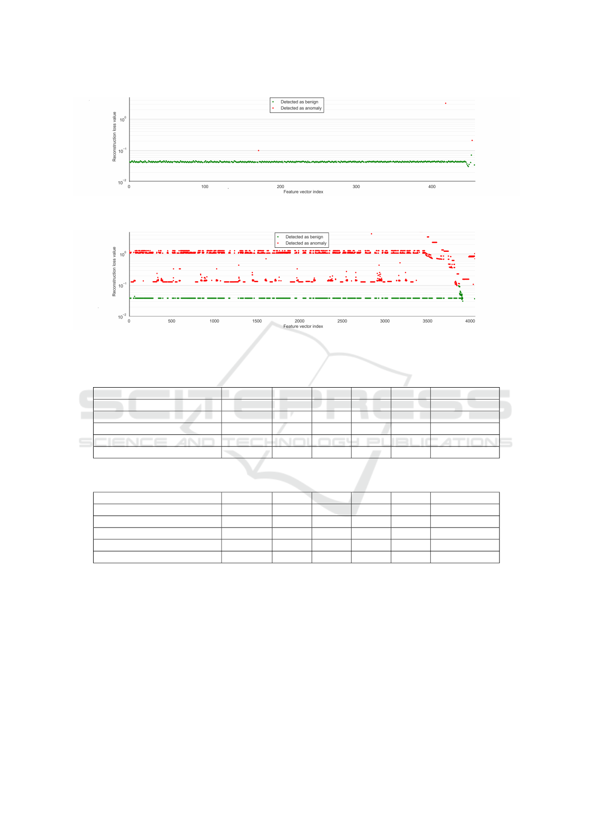
Figure 4: Reconstruction error of an AE for network data from a cross-site scripting (XSS) attack. The reconstruction error
from 444 feature vectors are below the anomaly detection threshold and 13 feature vectors are detected as anomaly.
Figure 5: Reconstruction error of an AE for network data from a Slowloris attack. The reconstruction error from 1102 feature
vectors are below the anomaly detection threshold and 2956 feature vectors are detected as anomaly.
Table 6: Comparison of evaluation results between VAE Prop and the two-stage approach for different filter factors (FF) for
the NSL-KDD dataset. The calculation time (in seconds) was measured for the evaluation of 22544 feature vectors.
Method Bal. Acc. Acc. Prec. Recall F1 Calc Time [s]
VAE Prob 0.8734 0.8744 0.8968 0.8806 0.8887 6.5326
AE CNN FF
0%
+ VAE Prob 0.8763 0.8768 0.9013 0.8800 0.8905 2.1912
AE CNN FF
1%
+ VAE Prob 0.8857 0.8837 0.9201 0.8714 0.8951 1.9588
AE CNN FF
5%
+ VAE Prob 0.8799 0.8768 0.9204 0.8578 0.8880 1.8052
AE CNN FF
10%
+ VAE Prob 0.8768 0.8729 0.9217 0.8488 0.8838 1.7513
Table 7: Comparison of evaluation results between VAE Prop and the two-stage approach for different filter factors (FF) for
the CICIDS-2017 dataset. The calculation time (in seconds) was measured for the evaluation of 1073893 feature vectors.
Method Bal. Acc. Acc. Prec. Recall F1 Calc Time [s]
VAE Prob 0.8523 0.9177 0.7508 0.7545 0.7526 139.1560
AE CNN FF
0%
+ VAE Prob 0.8537 0.9195 0.7587 0.7552 0.7570 100.6237
AE CNN FF
1%
+ VAE Prob 0.8542 0.9209 0.7660 0.7543 0.7601 81.6076
AE CNN FF
5%
+ VAE Prob 0.8551 0.9226 0.7739 0.7540 0.7638 64.0784
AE CNN FF
10%
+ VAE Prob 0.8567 0.9290 0.8098 0.7485 0.7779 43.9046
tice the goal is that an operator only has to analyse as
little suspicious data as possible.
An effect of the two-step approach is furthermore,
that the detected anomaly data was processed by two
methods, which leads to an increase of the precision.
The evaluation also showed that the threshold
value for anomaly detection for the respective meth-
ods is very different for the two datasets. The ex-
ception to this is VAE Prob, where, regardless of the
dataset and the type and number of features calcu-
lated, a similar threshold value was found to give the
best result in relation to metric F1.
The proposed method is only one part of the entire
semi-automatic intrusion detection process. Hence
in our future work we will also focus on the proper
preparation and presentation of detection results to
the operator. Conversely, the operator’s feedback
might serve as additional information for an adaptive
training of the second stage method. Another inter-
esting field or research will be the investigation of the
individual feature importance in the context of under-
standing and explainability of the system’s decisions
as well as the design of more discriminative and so-
phisticated features, because the runtime performance
ICISSP 2021 - 7th International Conference on Information Systems Security and Privacy
456

gain obtained by our approach will allow for
the usage of more complex network monitoring
features.
ACKNOWLEDGEMENTS
This work was funded by the Austrian Federal Min-
istry of Climate Action, Environment, Energy, Mobil-
ity, Innovation and Technology (BMK).
REFERENCES
Alshamrani, A., Myneni, S., Chowdhary, A., and Huang,
D. (2019). A Survey on Advanced Persistent Threats:
Techniques, Solutions, Challenges, and Research Op-
portunities. IEEE Communications Surveys Tutorials.
An, J. and Cho, S. (2015). Variational autoencoder based
anomaly detection using reconstruction probability.
Special Lecture on IE, 2:1–18.
Baddar, S. W. A.-H., Merlo, A., and Migliardi, M. (2014).
Anomaly detection in computer networks: A state-of-
the-art review. JoWUA, 5(4):29–64.
Chandola, V., Banerjee, A., and Kumar, V. (2009).
Anomaly Detection: A Survey. ACM computing sur-
veys (CSUR), 41(3):15.
Chen, J., Sathe, S., Aggarwal, C., and Turaga, D. (2017).
Outlier detection with autoencoder ensembles. In Pro-
ceedings of the 2017 SIAM International Conference
on Data Mining, pages 90–98. SIAM.
Duessel, P., Gehl, C., Flegel, U., Dietrich, S., and
Meier, M. (2017). Detecting zero-day attacks using
context-aware anomaly detection at the application-
layer. International Journal of Information Security,
16(5):475–490.
Fraley, J. B. and Cannady, J. (2017). The promise of
machine learning in cybersecurity. In SoutheastCon,
2017, pages 1–6. IEEE.
Ghafir, I., Hammoudeh, M., Prenosil, V., Han, L., Hegarty,
R., Rabie, K., and Aparicio-Navarro, F. J. (2018). De-
tection of advanced persistent threat using machine-
learning correlation analysis. Future Generation
Computer Systems, 89:349–359.
Hindy, H., Brosset, D., Bayne, E., Seeam, A., Tachtatzis,
C., Atkinson, R., and XavierBellekens (2018). A tax-
onomy and survey of intrusion detection systemdesign
techniques, network threats and datasets. Association
for Computing Machinery.
Hodo, E., Bellekens, X., Hamilton, A., Tachtatzis, C., and
Atkinson, R. (2017). Shallow and deep networks in-
trusion detection system: A taxonomy and survey.
arXiv preprint arXiv:1701.02145.
Javaid, A., Niyaz, Q., Sun, W., and Alam, M. (2016).
A deep learning approach for network intrusion de-
tection system. In Proceedings of the 9th EAI In-
ternational Conference on Bio-inspired Information
and Communications Technologies (formerly BIO-
NETICS), pages 21–26. ICST.
Kwon, D., Kim, H., Kim, J., Suh, S.-c., Kim, I., and Kim,
K. (2017). A survey of deep learning-based network
anomaly detection. Cluster Computing, pages 1–13.
Pawlicki, M., Chora
´
s, M., Kozik, R., and Hołubowicz, W.
(2020). On the impact of network data balancing in
cybersecurity applications. In International Confer-
ence on Computational Science, pages 196–210.
Ravi Kiran, M. T. and Parakkal, R. (2018). An overview
of deep learning based methods for unsupervised and
semi-supervised anomaly detection in videos. arXiv
preprint arXiv:1801.03149.
Ring, M., Wunderlich, S., Scheuring, D., Landes, D., and
Hotho, A. (2019). A survey of network-based in-
trusion detection data sets. Computers & Security,
86:147–167.
Schneider, P. and B
¨
ottinger, K. (2018). High-performance
unsupervised anomaly detection for cyber-physical
system networks. In CPS-SPC@CCS.
Sharafaldin, I., Lashkari, A. H., and Ghorbani, A. A.
(2018). Toward generating a new intrusion detection
dataset and intrusion traffic characterization. In 4th
International Conference on Information Systems Se-
curity and Privacy (ICISSP).
Stojanovi
´
c, B., Hofer-Schmitz, K., and Kleb, U. (2020).
Apt datasets and attack modeling for automated de-
tection methods: A review. Computers & Security,
92:101734.
Tavallaee, M., Bagheri, E., Lu, W., and Ghorbani, A. A.
(2009). A Detailed Analysis of the KDD CUP 99 Data
Set. In Proceedings of the 2009 IEEE Symposium on
Computational Intelligence.
Tuor, A., Kaplan, S., Hutchinson, B., Nichols, N., and
Robinson, S. (2017). Deep learning for unsuper-
vised insider threat detection in structured cybersecu-
rity data streams. arXiv preprint arXiv:1710.00811.
Xin, Y., Kong, L., Liu, Z., Chen, Y., Li, Y., Zhu, H., Gao,
M., Hou, H., and Wang, C. (2018). Machine learning
and deep learning methods for cybersecurity. IEEE
Access, 6:35365–35381.
Y
¨
uksel,
¨
O., den Hartog, J., and Etalle, S. (2016). Reading
between the fields: practical, effective intrusion detec-
tion for industrial control systems. In Proceedings of
the 31st Annual ACM Symposium on Applied Comput-
ing, pages 2063–2070. ACM.
Zavrak, S. and Iskefiyeli, M. (2020). Anomaly-Based In-
trusion Detection From Network Flow Features Us-
ing Variational Autoencoder. IEEE Access, 8:108346–
108358.
Two Stage Anomaly Detection for Network Intrusion Detection
457
