
A Framework of Hierarchical Deep Q-Network for Portfolio
Management
Yuan Gao
1,?
, Ziming Gao
1,?
, Yi Hu
1
, Sifan Song
1
, Zhengyong Jiang
1
and Jionglong Su
2
1
Department of Mathematical Sciences, Xi’an Jiaotong - Liverpool University, Suzhou, P. R. China
2
School of AI and Advanced Computing, XJTLU Entrepreneur College (Taicang), Xi’an Jiaotong - Liverpool University,
Keywords:
Q-Learning, Hierarchical Reinforcement Learning, Convolutional Neural Network, Portfolio Management.
Abstract:
Reinforcement Learning algorithms and Neural Networks have diverse applications in many domains, e.g.,
stock market prediction, facial recognition and automatic machine translation. The concept of modeling the
portfolio management through a reinforcement learning formulation is novel, and the Deep Q-Network has
been successfully applied to portfolio management recently. However, the model does not take into account
of commission fee for transaction. This paper introduces a framework, based on the hierarchical Deep Q-
Network, that addresses the issue of zero commission fee by reducing the number of assets assigned to each
Deep Q-Network and dividing the total portfolio value into smaller parts. Furthermore, this framework is
flexible enough to handle an arbitrary number of assets. In our experiments, the time series of four stocks
for three different time periods are used to assess the efficacy of our model. It is found that our hierarchical
Deep Q-Network based strategy outperforms ten other strategies, including nine traditional strategies and one
reinforcement learning strategy, in profitability as measured by the Cumulative Rate of Return. Moreover, the
Sharpe ratio and Max Drawdown metrics both demonstrate that the risk of policy associated with hierarchical
Deep Q-Network is the lowest among all ten strategies.
1 INTRODUCTION
Profitable stock trading strategy is a process of mak-
ing decisions based on optimizing allocation of cap-
ital into different stocks in order to maximize per-
formance, such as expected return and Sharpe ra-
tio (Sharpe, 1994). Traditionally, there exist port-
folio trading strategies which may be broadly clas-
sified into four categories, namely “Follow-the-
Winner”, “Follow-the-Loser”, “Pattern-Matching”,
and “Meta-Learning” (Li and Hoi, 2014). However,
in real financial environments with complex correla-
tions between stocks as well as substantially noisy
data, such traditional portfolio trading strategies tend
to be limited in their usefulness.
To date, several deep machine-learning ap-
proaches have been applied to financial trading (Park
et al., 2019) with varying degrees of success. Nev-
ertheless, many of them tend to predict price move-
ments by inputting historical asset prices to output a
prediction of asset prices in next trading period via
?
These authors contribute equally to this work.
neural network, and the trading agent will take action
based on these predictions (Heaton et al., 2016). The
performance of these algorithms is highly dependent
on the accuracy of future market prices, and it seems
inappropriate to convert price predictions into actions
because they are not part of the market actions. There-
fore, these approaches are not fully machine learning
based.
More recently, the applications of Reinforcement
Learning (RL) methods in portfolio management are
proposed, where these approaches are able to trade
without predicting future prices (Dempster and Lee-
mans, 2006). Most of these are related to policy-based
RL such as Policy Gradient (Jiang et al., 2017), which
are suitable for continuous actions in the stock sce-
nario. However, with appropriate action discretiza-
tion in stock trading, several valued-based RL meth-
ods such as Q-Learning have been applied as well.
In (Gao et al., 2020), a Deep Q-Network (N-DQN)
framework combining Q-Learning with a single deep
neural network has been proposed. This framework
allows the N-DQN agent to optimize trading strate-
gies through learning from its experience in the finan-
132
Gao, Y., Gao, Z., Hu, Y., Song, S., Jiang, Z. and Su, J.
A Framework of Hierarchical Deep Q-Network for Portfolio Management.
DOI: 10.5220/0010233201320140
In Proceedings of the 13th International Conference on Agents and Artificial Intelligence (ICAART 2021) - Volume 2, pages 132-140
ISBN: 978-989-758-484-8
Copyright
c
2021 by SCITEPRESS – Science and Technology Publications, Lda. All rights reserved

cial environment, so that this agent may adapt strate-
gies derived from historical data to actual trading.
Nevertheless, the single DQN structure of the N-DQN
is unable to handle extremely large action space, and
large capital sectors will lead to higher commission
fee during trading process. Therefore, the algorithm
in (Gao et al., 2020) makes an unrealistic assumption
of zero commission fee.
In this paper, we address this shortcoming by
adopting hierarchical DQN structure (Kulkarni et al.,
2016) to obtain a novel hierarchical Deep Q-Network
(H-DQN) which takes into consideration of commis-
sion fee in transaction. It successfully decreases the
number of assets assigned to each DQN and reduces
the number of actions. Thus, the problem associated
with high commission fee is solved and the function-
ality of the algorithm is greatly improved. To the best
of our knowledge, the application of DQN to port-
folio management with the consideration of commis-
sion fee is entirely novel.
Our key contributions are two-fold. first, we re-
duce the action space by proposing a H-DQN frame-
work so that we no longer assume zero commission
fee during transaction. Second, we construct the in-
teracting environment between the framework and the
market as well as the interacting environment inside
the framework, thereby enabling the model to adapt
to real-world trading process.
The rest of this paper is organized as follows. Sec-
tion 2 defines the portfolio management problem in
this research. All the assumptions made in this study
are listed in Section 3. Section 4 gives the network
architecture. Data processing and interacting pro-
cess are given in Section 5. Section 6 presents the
training process of the H-DQN model. Experiments
and results are given in Section 7. Finally, Section 8
gives the conclusions and research directions for fu-
ture work.
2 PROBLEM STATEMENT
In portfolio management, we seek the optimal invest-
ment policy that gives the maximum overall portfo-
lio over a given period of time. In practice, adjusted
weight of portfolio in different assets are based on
the price of the assets and the previous weight of the
portfolio. This process can be described as Markov
Decision Process (MDP) (Neuneier, 1998). Essen-
tially, the MDP is a mathematical model used to de-
velop an optimal strategy, which consists of a tuple
(S
t
, a
t
, P
t
, R
t
). The meaning of each element in the tu-
ple is given as follows:
• S
t
- the state at time t;
• a
t
- the action taken at time t;
• P
t
- the probability of state transiting from S
t
to
S
t+1
;
• R
t
- the reward at time t.
In order to construct the MDP model for portfolio
management, we define the state at time t, S
t
, to be the
price of investment products, and the action of time t
as:
a
t
, w
t
(1)
where w
t
is the weight vectors of portfolio at time t.
Motivated by action discretized method (Gao et al.,
2020), we divide the portfolio value equally into N
parts, then consider these parts as the smallest trading
units in portfolio management and allocate them to to-
tal assets M + 1 (including cash). Therefore, we may
discretize the action space, and then the total number
of actions equals
M+N
M
, calculated by permutation,
where M is the number of assets. In addition, we de-
fine the reward at time t as:
R
t
, p
t+1
− p
t
(2)
where p
t
and p
t+1
are respectively the portfolio value
at time t and t + 1.
In (2), we only focus on the reward at the current
time t, whereas the state of time t caused by the given
policy π affects all the states after time t, i.e., the value
of S
t
is not only current reward R
t
, but also the re-
wards of subsequent time periods. Therefore, with
policy π, the value function, G
π
, of state S
t
should be
defined as:
G
π
(S
t
) ,
T
∑
k=t
γ
k−t
R
k
(3)
where T denotes the last trading period and γ ∈ (0, 1]
is the discount factor. In general, it is very com-
plicated to calculate G
π
(S
t
) using (3), so we need
to compute the expectation of G
π
to approximate its
true value. Furthermore, since the policy π is defined
solely by action a
t
, we define the value function Q
π
of S
t
and a
t
as:
Q
π
(S
t
, a
t
) , E[G
π
(S
t
)]
(4)
which is the basic principle of Q Learning. Com-
bining the basic principle and neuro network, we can
build a Deep Q-Network (DQN) that can solve prob-
lems with infinite state space, e.g., portfolio manage-
ment. However, in the above description, we find that
the number of actions increases with the increment of
number of parts that we divide the total portfolio into,
and the number of assets. Moreover, if we decrease
the number of parts N in order to reduce the number
of actions, the trading unit will be larger, which may
result in large commission fee as a result of frequent
A Framework of Hierarchical Deep Q-Network for Portfolio Management
133

Figure 1: Structure of DQNs.
Figure 2: Structure of controllers.
trading. Therefore, we shall reduce the number of as-
sets M handled by each DQN so that trading unit can
be small enough to avoid the problem caused by large
commission fee.
3 ASSUMPTIONS
Before introducing the model, we shall make the fol-
lowing simplifying assumptions:
1. The action taken by the agent will not affect the
financial market such as the price and volume.
2. Other than the commission fee deducted during
transition process, the portfolio value remains un-
changed between the end of previous trading pe-
riod and the beginning of next trading period.
3. The agent can not invest money into assets other
than the selected ones.
4. The volume of each stock is large enough for the
agent to buy or sell each of them at any trading
day.
5. The transition process is short enough so that the
time for this process may be ignored.
4 NETWORK ARCHITECTURE
In this section, we shall introduce the architecture of
H-DQN (Fig.7) that can handle an arbitrary number
of assets, e.g., stocks, cash etc. As mentioned in Sec-
tion 2, to solve the problem associated with commis-
sion fee, the total portfolio value should be divided
into smaller parts, which leads to large action space.
Therefore, we shall decrease the number of assets as-
signed to the DQN. To achieve this, we consider sev-
eral independent DQNs in the system. Each DQN has
identical structure and is responsible for three assets
(one cash and two stocks) so that the number of as-
sets each DQN is smaller than that of traditional DQN
which deals with large number of assets. Next, we de-
fine a controller which is actually a DQN whose struc-
ture is different from the DQNs interacting with mar-
ket. Considering that controller is also a DQN, i.e., its
action space should be limited as well, we assign two
DQNs to the controller. Furthermore, for each con-
troller, there is a controller of higher level to control
it. Consequently, we obtain the general structure of
H-DQN.
From now on, we shall focus on a structural unit of
H-DQN (Fig.3) since the network topology and trad-
ing process of the general structure can be general-
ized from its structural unit. In Fig.3, we see that the
controller divides the total portfolio into three parts,
i.e., cash, the portfolio managed by DQN1 and the
portfolio managed by DQN2. As such, the DQNs on
the lower level receive the portfolio for investing in
the market. The specific trading process will be intro-
duced in section 6.
The network topologies of the DQNs and con-
trollers are inspired by (Jiang et al., 2017). In our
network, we change the structure of dense layers in
(Jiang et al., 2017) and make it a dueling Q-net.
We shall first describe the topology of the DQNs, as
shown in Fig.1.
(1) Input and Output: The input of DQNs is the
state S
t
of last trading period, which is defined by
S
t
, (P
t
, w
t−1
)
s.t.
w
t−1
= (w
t−1,0
, w
t−1,1
, w
t−1,2
)
P
t
=
P
o
t
, P
c
t
, P
h
t
, P
l
t
(5)
where w
t−1
, i = 0, 1, 2 denotes the proportion of port-
folio value assigned to this DQN that invested in the
i
th
stock at the beginning of previous trading period.
ICAART 2021 - 13th International Conference on Agents and Artificial Intelligence
134
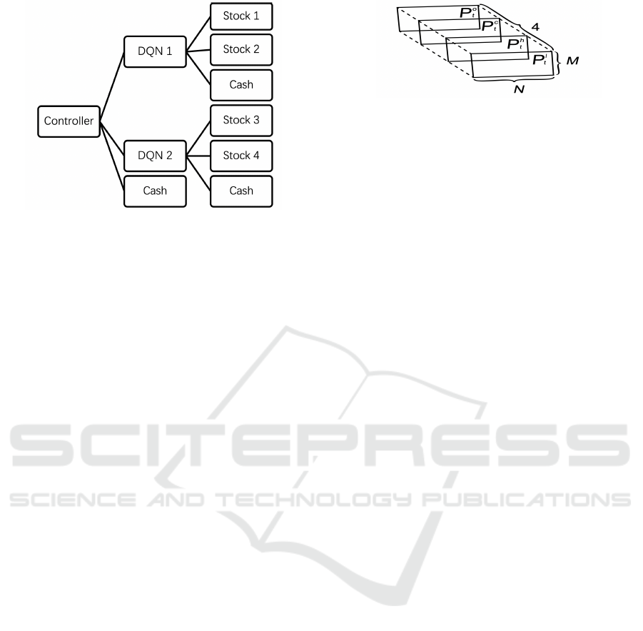
Figure 3: Architecture of structural unit in H-DQN.
Moreover, we initialize w
0
(weight vector at the be-
ginning of the episode) as
w
0
= (1, 0, 0) (6)
i.e., all the portfolio value is in form of cash. P
t
is the
price tensor of the previous N trading days (defined
in Section 5.1). What should be mentioned is that the
number of stocks M equals 2 because each DQN only
holds 2 stocks in our hierarchical model shown in Fig.
1. The output of DQN is w
t
, the weight vector at the
beginning of next trading period.
(2) 1st and 2nd CNN Layers: As shown in Fig. 1,
the first CNN layer receives the price tensor P
t
with
dimension (2, 10, 4). The filter of this layer is in size
of 1 × 3, and the activation function we use here is
Selu which is defined in (Klambauer et al., 2017). In
this layer, we obtain 32 feature maps and each one is
in size of 2 × 5, and these feature maps are received
by the next CNN layer. In the second CNN layer,
the filters are of size 1 × 5 and 64 feature maps are
produced.
(3) Weight Insertion and 3rd CNN Layer: In the
layers mentioned above, we only extract features from
the price tensor, but the weight vector w
t−1
has not
been used. So after obtaining 64 feature maps from
the second CNN layer, we insert the weight vector
w
t−1
(with the weight of cash removed) into these fea-
ture maps and produce a tensor with dimension (2, 1,
65). In the third CNN layer, the size of filter is 1 × 1
and 128 feature maps are produced, following which
the 128 features are flattened and a cash bias (Jiang
et al., 2017) (a 1 × 1 tensor with value 1) is added
onto the flattened feature map.
(4) Dense Layers: Every neuro in the first dense
layer receives the flattened features and connects with
each neuro in next dense layer. In the second dense
layer, we use the structure called dueling Q-net (Wang
et al., 2016), which consists of state layer and action
layer. With this structure, the value of state and the
Figure 4: Original price tensor P
∗
t
.
value of actions may be estimated separa(Wang et al.,
2016)tely. After the Q-value of state Q
s
and Q-value
of each action Q
a
are obtained, we can compute the
final Q-value of each action by where E[Q
a
] is the
expectation of Q-values of actions.
Q
(S
t
,a)
= Q
s
+ (Q
a
− E [Q
a
]) (7)
The structure of controller is similar to DQNs, which
is given in Fig.2. The main difference lies in the con-
volutional layers. Since the price tensor received here
is M × N × 4 but the weight is still a 2 × 1 (with first
element removed) vector, i.e. the first dimension may
not be equal, so we cannot insert the weight into the
feature maps. Therefore, we flatten the feature maps
after the first and second convolution layers and con-
catenate the weight to it. Finally, we input the flat-
tened feature map into the remaining network which
is also a dueling Q-net.
5 MATHEMATICAL
FORMALISM
5.1 Data Processing
Considering that the raw price data cannot be received
by the network directly, we need to process the data
and transform it to a ’tensor’ structure.
For the price tensor P
t
, it is converted from the
original price tensor P
∗
t
consisting of P
o
t
, P
c
t
, P
h
t
, P
l
t
which are the normalized price matrices of opening,
closing, highest and lowest as denoted below:
P
o
t
=
p
o
t−n+1
p
c
t
|. . . |p
o
t
p
c
t
(8)
P
c
t
=
p
c
t−n+1
p
c
t
|. . . |p
c
t
p
c
t
(9)
P
h
t
=
h
p
h
t−n+1
p
c
t
|. . . |p
h
t
p
c
t
i
(10)
P
l
t
=
h
p
l
t−n+1
p
c
t
|. . . |p
l
t
p
c
t
i
(11)
where is elementwise division. In addition,
P
o
t
, P
c
t
, P
h
t
, P
l
t
represent the price vectors of opening,
closing, highest and lowest price for all assets in trade
period t respectively. In other words, the i
th
element
A Framework of Hierarchical Deep Q-Network for Portfolio Management
135

Figure 5: Transaction process.
of them, p
o
t,i
, p
c
t,i
, p
h
t,i
, p
l
t,i
, are relative technical indi-
cators of i
th
asset in the i
th
period. Therefore, if there
are M assets (except cash) in the portfolio, the origi-
nal price tensor P
∗
t
is an (M, N, 4)-dimensional tensor,
as illustrated in Fig. 4
We note that simply normalizing the original ten-
sor price may trigger some recognition problems, i.e.,
the features of normalized original price tensors are so
similar that the network may not distinguish between
them and determine which action should be taken. In
view of this, each element in P
∗
t
should be reduced by
1 and multiplied by an expansion coefficient α to en-
hance the features of the price tensor. Therefore, the
final price tensor is defined as:
P
t
, α (P
∗
t
− 1) (12)
where 1 is a tensor of dimension of (M, N, 4), whose
elements are all 1’s.
Because the controllers and the DQNs (Fig.3)
have similar structure, we may process the data re-
ceived by DQNs using same method discussed in this
section. The dimension of price tensor and weight
vector of bottom DQNs are of size (2, N, 4) and 1 × 3
respectively, since each bottom DQN can only handle
2 stocks and cash.
5.2 Interaction with Environment
As mentioned in Section 4, the structure of the system
is hierarchical which consists of controllers and bot-
tom DQNs. Since the controllers have similar proper-
ties, we shall introduce the interacting process of one
controller and the DQNs corresponding to it (Fig.3)
instead of the interacting process of the whole system.
The interaction process is shown in Fig. 5.
The interaction process starts with the controller
receiving the state S
t
as defined in (5), and giving the
weight vector w
∗
t
, where the weight vector represents
the proportion of portfolio conserved as cash and as-
signed to the bottom DQNs. This relocation of port-
folio incurs commission fee c
1
defined as:
c
1
= dy
0
t−1
2
∑
i=1
w
∗
t,i
− w
0
t−1,i
(13)
where d is the commission rate. The notation y
0
t−1
and
w
0
t−1
are respectively the portfolio value and weight
at the end of the trading period t − 1. Moreover, we
omit the weight of cash here because the change of
cash does not incur commission fee.
Next, the DQNs of next level receive the state
S
t,1
, S
t,2
respectively and output w
1,t
, w
2,t
. The com-
mission fee of this relocation of portfolio is given by
c
2
= d
y
0
t−1
− c
1
(w
∗
t,1
2
∑
i=1
w
1,t,i
− w
0
1,t−1,i
+
w
∗
t.2
2
∑
i=1
w
2,t,i
− w
0
2,t−1,i
)
(14)
So far, we obtain the portfolio value at the beginning
of next trading period as:
y
t
= y
0
t−1
− c
1
− c
2
(15)
The portfolio value held by DQN1 and DQN2 are
given respectively by
y
1,t
= w
∗
t,1
y
0
t−1
− c
1
1 − d
2
∑
i=1
w
1,t,i
− w
0
1,t−1,i
!
y
2,t
= w
∗
t,2
y
0
t−1
− c
1
1 − d
2
∑
i=1
w
2,t,i
− w
0
2,t−1,i
!
(16)
and weight vectors of DQNs at the beginning of next
trading period are w
1,t
and w
2,t
.
However, the weight vector of the controller at
the beginning of the next trading period is not sim-
ply given by w
∗
t
, since the portfolio value assigned to
DQNs is changed after interacting with market, i.e.,
commission fee is deducted. Therefore, the weight
vector of controller at the beginning of next trading
period is the proportion of portfolio value after the
transition, given by
w
t
=
w
∗
t,0
y
0
t−1
− c
1
y
t
,
y
1,t
y
t
,
y
2,t
y
t
!
(17)
Then, during the next trading period, the price rela-
tive vector of assets assigned to DQN1 and DQN2 are
given by
µ
µ
µ
∗
1,t
= p
o
1,t+1
p
o
1,t
=
p
o
1,t+1,1
p
o
1,t,1
,
p
o
1,t+1,2
p
o
1,t,2
, . . . ,
p
o
1,t+1,m
p
o
1,t,m
!
µ
µ
µ
∗
2,t
= p
p
p
o
2,t+1
p
p
p
o
2,t
=
p
o
2,t+1,1
p
o
2,t,1
,
p
o
2,t+1,2
p
o
2,t,2
, . . . ,
p
o
2,t+1,m
p
o
2,t,m
!
(18)
ICAART 2021 - 13th International Conference on Agents and Artificial Intelligence
136

Here, we define the time of opening quotation as the
demarcation point of previous and next trading pe-
riod, i.e., the previous trading period is before the
point and next trading period is after the point, and
by Section 3 Assumption 5, all the transition activi-
ties take place in a very short period of time after the
opening quotation. Moreover, since the total portfo-
lio value includes cash, we need to add cash price to
µ
µ
µ
∗
1,t
and µ
µ
µ
∗
2,t
. Considering the fact that the cash price
remains unchanged, µ
µ
µ
1,t
and µ
µ
µ
2,t
would take the fol-
lowing form
µ
µ
µ
1,t
=
1,
p
o
1,t+1,1
p
o
1,t,1
,
p
o
1,t+1,2
p
o
1,t,2
, . . . ,
p
o
1,t+1,m
p
o
1,t,m
!
µ
µ
µ
2,t
=
1,
p
o
2,t+1,1
p
o
2,t,1
,
p
o
2,t+1,2
p
o
2,t,2
, . . . ,
p
o
2,t+1,m
p
o
2,t,m
!
(19)
and the portfolio value of DQN1 and DQN2 at the end
of next trading period are given by
y
0
1,t
= y
1,t
w
w
w
1,t
µ
µ
µ
T
1,t
y
0
2,t
= y
2,t
w
w
w
2,t
µ
µ
µ
T
2,t
(20)
Therefore, the total portfolio value is
y
0
t
= w
∗
t,0
y
0
t−1
− c
1
+ y
0
1,t
+ y
0
2,t
(21)
Using the portfolio value at the end of next and pre-
vious trading period, we may calculate the reward of
controller and reward of DQNs as
r
t
= log
y
0
t
y
0
t−1
!
r
1,t
= log
y
0
1,t
y
0
1,t−1
!
r
2,t
= log
y
0
2,t
y
0
2,t−1
!
(22)
6 TRAINING PROCESS
Since the controllers and DQNs are all Deep Q-
networks essentially, their parameters may be updated
by general training process of DQN. For this model,
we applied the training process that is widely used in
Double Deep Q-network (Van Hasselt et al., 2015).
Considering that the basic principle of DQN is
to approximate the real Q-function, there should be
two Deep Q-Networks, i.e., the evaluation network
Q
eval
and the target network Q
target
, which have ex-
actly same structure but different parameters. The pa-
rameters of Q
eval
are continuously updated, while the
parameters of Q
target
are fixed until they are replaced
by the parameters of Q
eval
.
Algorithm 1: Training process.
Input: Batch size N, Target network Q
θ
∗
Input: Estimation network Q
θ
, Target vector v
tar
Input: Estimation vector v
est
, Real value vector v
real
1: for i = 1 → N do
2: Take sample (S
t
i
, a
t
i
, r
t
i
, S
t
i
+1
)
3: v
tar
(i) = Q
θ
∗
(S
t
i
+1
, argmax
a
(Q
θ
(S
t
i
+1
, a)))
4: v
est
(i) = Q
θ
(S
t
i
, argmax
a
(Q
θ
(S
t
i
, a)))
5: if S
t
i
+1
is terminal then
6: v
real
(i) = r
t
i
7: else
8: v
real
(i) = r
t
i
+ γv
tar
(i), γ ∈ (0, 1]
9: end if
10: end for
11: Do a gradient decent step with
k
v
real
− v
est
k
2
12: Replace the parameter of target net θ
∗
← θ
7 EXPERIMENT
7.1 Experimental Setting
In our experiment, four low-correlation stocks in Chi-
nese A-share market, codes of which are 600260,
600261, 600262, 600266 respectively, are chosen
as risk assets (downloaded from tushare). Com-
bined with the cash as risk-free asset, there are
a total of five investment assets to be managed.
In order to increase the difference between price
tensors, we set the trading period as two days.
Meanwhile, we set 2011/1/1-2012/12/31, 2014/1/1-
2015/12/31, 2015/1/1-2016/12/31 as the period of
training set and 2013/1/14-2013/12/19, 2016/1/14-
2016/12/19, 2017/1/13-2017/12/18 as the period of
back-test intervals. The same hyperparameters were
used in the above three experiments.
7.2 Performance Metrics
This section presents three different financial metrics
for evaluating the performance of trading strategies.
The first metric is the cumulative rate of return (CRR)
(Jiang et al., 2017), defined as:
CRR = exp
T
∑
t=1
r
t
!
− 1 (23)
where T is the total number of trading periods and r
t
is
the reward in t
th
period as defined in (22). This metric
may be used to evaluate the profitability of strategies
directly.
The second metric, the Sharpe ratio (SR), is
mainly used to assess the risk-adjusted return of
strategies (Sharpe, 1994). It is defined as:
A Framework of Hierarchical Deep Q-Network for Portfolio Management
137

Figure 6: Trading performance in three back-test intervals.
SR =
E[ρ
t
− ρ
RF
]
p
Var (ρ
t
− ρ
RF
)
(24)
where E and Var are the expectation and variance re-
spectively. The notation ρ
t
is the rate of return defined
as:
ρ
t
,
y
0
t
y
0
t−1
− 1 (25)
Here, y
0
t
, y
0
t−1
are portfolio value at the end of t
th
pe-
riod and t − 1
th
period. The parameter ρ
RF
represents
the rate of return of risk-free asset.
To evaluate an investment strategy’s risk toler-
ance, we introduce Maximum Drawdown (Magdon-
Ismail and Atiya, 2004) as the third metric. The for-
mula of Maximum Drawdown (MDD) is
MDD = max
β>t
y
t
− y
β
y
t
(26)
This metric denotes the maximum portfolio value loss
from a global maximum to global minimum so that
we can measure the largest possible loss using it.
7.3 Result and Analysis
The performance of trading strategy is compared with
several strategies as listed below (each strategy is
tested with commission rate of 0.25%), and these
strategies can be categorized into two types:
Type I. Traditional trading strategies
• Robust Median Reversion (RMR) (Huang et al.,
2012)
• Uniform Buy and Hold (BAH) (Li and Hoi, 2014)
• Universal Portfolios (UP) (Cover, 2011)
• Exponential Gradient (EG) (Helmbold et al.,
1998)
• Online Newton Step (ONS) (Agarwal et al., 2006)
• Aniticor (ANTICOR) (Borodin et al., 2004)
• Passive Aggressive Mean Reversion (PAMR) (Li
et al., 2012)
• Online Moving Average Reversion (OLMAR) (Li
et al., 2015)
• Confidence Weighted Mean Reversion (CWMR)
(Li et al., 2013)
Type II. Reinforcement learning trading strategy
• Single DQN (N-DQN), an approach combining
Q-learning with a single deep neural network with
commission fee taken into consideration (com-
mission rate of 0.25%) (Gao et al., 2020)
The first dataset gives the cumulative return over the
investment horizon of the test period as learning con-
tinuous from 2013/01/14 to 2013/12/19. Overall, the
H-DQN strategy outperforms all other strategies in
contrast to N-DQN strategy which does not perform
as well as benchmarks such as OLMAR and ANTI-
COR. Although the advantage of H-DQN strategy is
not apparent at the beginning, and the disparity be-
tween H-DQN strategy and other strategies becomes
obvious especially in the last 1/3 of the trading period.
Compared to N-DQN strategy which shows fluctua-
tions along the time periods, H-DQN strategy tends
to increase over the test trading period in general and
the cumulative return is almost always above the ini-
tial cashflow.
Similarly, in the second dataset test which is
from 2016/01/14 to 2016/12/19, the cumulative return
shows that the H-DQN strategy has the best perfor-
mance among all the strategies in the scenario that N-
DQN shows no outstanding performance. In addition,
the H-DQN strategy outperforms other strategies for
the most of the time periods, and the difference be-
tween H-DQN strategy and other benchmarks is sig-
nificant in the latter half of the time periods. Com-
pared to the total portfolio value which remains at a
low level as demonstrated by other strategies, the total
portfolio value of H-DQN strategy tends to increase
over the test trading period in general and the cumu-
lative return is obviously higher than others for most
of the time periods.
The third dataset gives the cumulative return
over the test periods from 2017/01/05 to 2017/11/17.
Again, the H-DQN strategy outperforms benchmark
strategies for the majority of the test trading period,
and begins to perform very well halfway through the
trading period. Compared to N-DQN strategy which
shows moderate increase, the H-DQN strategy tend to
increase over the test trading period in general and the
overall increase is much higher than N-DQN.
ICAART 2021 - 13th International Conference on Agents and Artificial Intelligence
138
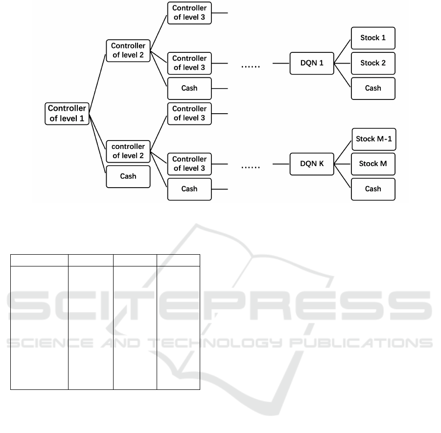
Figure 7: General architecture of H-DQN.
Table 1: Average Performance of Eleven Strategies.
CRR SR MDD
RMR -12.84% -4.00% 22.98%
BAH 3.97% 1.97% 17.78%
UP -9.12% -2.35% 24.38%
EG -1.93% -0.22% 17.43%
ONS -8.16% -1.48% 26.16%
ANTICOR -2.98% -2.17% 19.89%
PAMR -9.83% -4.11% 23.04%
OLMAR -9.55% -5.26% 24.34%
CWMR -3.84% -2.32% 20.36%
N-DQN 8.19% 2.72% 22.72%
H-DQN 44.37% 10.33% 11.69%
Table 1 gives the average performance of hierarchi-
cal DQN strategy and benchmarks over three test sets
based on the metrics CRR, SR and MDD. It is obvi-
ous that the numerical results of H-DQN strategy are
the best in all aspects. In the case of CRR, the re-
sult of H-DQN strategy (44.37%) exceeds the second
highest benchmark N-DQN (8.19%) by 36%. As for
the risk measure, the H-DQN strategy still gives the
best performance with minimum MDD (11.69%), as
compared to the EG benchmark (17.43%). For SR,
H-DQN strategy (10.33%) outperforms the next best
performing strategy N-DQN benchmark (2.72%). It
should be noted that N-DQN is also a reinforcement
learning algorithm, but without the hierarchical archi-
tecture, its performance is much worse than H-DQN.
Overall, the results in all three back-test intervals
demonstrate the good profitability and adaptability of
H-DQN framework in comparison to N-DQN and all
other traditional strategies.
8 CONCLUSIONS AND FUTURE
WORK
In this paper, we construct a hierarchical reinforce-
ment learning framework that can handle an arbitrary
number of assets for portfolio management which
takes commission fee into consideration. Four stocks
are selected as our experimental data, and Cumula-
tive Rate of Return, Sharpe ratio, Maximum Draw-
down are used to compare the profitability and risk
of our model in the back-test intervals against nine
traditional strategies as well as the single DQN strat-
egy. The results show that this hierarchical reinforce-
ment learning algorithm outperforms all the other ten
strategies, and it is also the least risky investment
method our back-test intervals.
However, there are three major limitations. First,
since the controller on higher level needs to manage
more controllers, it is more difficult to train. Sec-
ond, we assume that the volumes of stocks are large
enough so each stock is available on any trading day.
However, the stock might not be available sometimes,
which will therefore impact the profit. Finally, for
generalization, our strategies will be vulnerable due to
a small mismatch between the learning environment
and the testing environment.
For future work, considering that deep reinforce-
ment learning algorithm is highly sensitive to the
noise in data, we may use traditional approaches to re-
duce financial data noise, e.g., wavelet analysis (Rua
and Nunes, 2009) and the Kalman Filter (Faragher,
2012). Moreover, as the number of assets increases,
there will be more controllers and DQNs in the hierar-
A Framework of Hierarchical Deep Q-Network for Portfolio Management
139

chical structure (shown in Fig.7), which may require a
long training period. To address this, we will look into
proposing new training methods that may improve the
efficiency in training the network.
REFERENCES
Agarwal, A., Hazan, E., Kale, S., and Schapire, R. E.
(2006). Algorithms for portfolio management based
on the newton method. In Proceedings of the 23rd
international conference on Machine learning, pages
9–16.
Borodin, A., El-Yaniv, R., and Gogan, V. (2004). Can we
learn to beat the best stock. In Advances in Neural
Information Processing Systems, pages 345–352.
Cover, T. M. (2011). Universal portfolios. In The Kelly Cap-
ital Growth Investment Criterion: Theory and Prac-
tice, pages 181–209. World Scientific.
Dempster, M. A. and Leemans, V. (2006). An automated fx
trading system using adaptive reinforcement learning.
Expert Systems with Applications, 30(3):543–552.
Faragher, R. (2012). Understanding the basis of the kalman
filter via a simple and intuitive derivation [lecture
notes]. IEEE Signal processing magazine, 29(5):128–
132.
Gao, Z., Gao, Y., Hu, Y., Jiang, Z., and Su, J. (2020). Appli-
cation of deep q-network in portfolio management. In
2020 5th IEEE International Conference on Big Data
Analytics (ICBDA), pages 268–275. IEEE.
Heaton, J., Polson, N. G., and Witte, J. H. (2016). Deep
learning in finance. arXiv preprint arXiv:1602.06561.
Helmbold, D. P., Schapire, R. E., Singer, Y., and Warmuth,
M. K. (1998). On-line portfolio selection using mul-
tiplicative updates. Mathematical Finance, 8(4):325–
347.
Huang, D., Zhou, J., Li, B., HOI, S., and Zhou, S. (2012).
Robust median reversion strategy for on-line portfo-
lio selection.(2013). In Proceedings of the Twenty-
Third International Joint Conference on Artificial In-
telligence: IJCAI 2013: Beijing, 3-9 August 2013.
Jiang, Z., Xu, D., and Liang, J. (2017). A deep re-
inforcement learning framework for the financial
portfolio management problem. arXiv preprint
arXiv:1706.10059.
Klambauer, G., Unterthiner, T., Mayr, A., and Hochre-
iter, S. (2017). Self-normalizing neural networks. In
Advances in neural information processing systems,
pages 971–980.
Kulkarni, T. D., Narasimhan, K., Saeedi, A., and Tenen-
baum, J. (2016). Hierarchical deep reinforcement
learning: Integrating temporal abstraction and intrin-
sic motivation. In Advances in neural information pro-
cessing systems, pages 3675–3683.
Li, B. and Hoi, S. C. (2014). Online portfolio selection: A
survey. ACM Computing Surveys (CSUR), 46(3):1–
36.
Li, B., Hoi, S. C., Sahoo, D., and Liu, Z.-Y. (2015). Moving
average reversion strategy for on-line portfolio selec-
tion. Artificial Intelligence, 222:104–123.
Li, B., Hoi, S. C., Zhao, P., and Gopalkrishnan, V. (2013).
Confidence weighted mean reversion strategy for on-
line portfolio selection. ACM Transactions on Knowl-
edge Discovery from Data (TKDD), 7(1):1–38.
Li, B., Zhao, P., Hoi, S. C., and Gopalkrishnan, V. (2012).
Pamr: Passive aggressive mean reversion strategy for
portfolio selection. Machine learning, 87(2):221–258.
Magdon-Ismail, M. and Atiya, A. F. (2004). Maximum
drawdown. Risk Magazine, 17(10):99–102.
Neuneier, R. (1998). Enhancing q-learning for optimal as-
set allocation. In Advances in neural information pro-
cessing systems, pages 936–942.
Park, S., Song, H., and Lee, S. (2019). Linear programing
models for portfolio optimization using a benchmark.
The European Journal of Finance, 25(5):435–457.
Rua, A. and Nunes, L. C. (2009). International comovement
of stock market returns: A wavelet analysis. Journal
of Empirical Finance, 16(4):632–639.
Sharpe, W. F. (1994). The sharpe ratio. Journal of portfolio
management, 21(1):49–58.
Van Hasselt, H., Guez, A., and Silver, D. (2015). Deep
reinforcement learning with double q-learning. arXiv
preprint arXiv:1509.06461.
Wang, Z., Schaul, T., Hessel, M., Hasselt, H., Lanctot, M.,
and Freitas, N. (2016). Dueling network architectures
for deep reinforcement learning. In International con-
ference on machine learning, pages 1995–2003.
ICAART 2021 - 13th International Conference on Agents and Artificial Intelligence
140
