
Pricing Competition in a Duopoly with Self-adapting Strategies
Youri Kaminsky, Tobias Maltenberger, Mats P
¨
orschke, Jan Westphal and Rainer Schlosser
Hasso Plattner Institute, University of Potsdam, Potsdam, Germany
Keywords:
Dynamic Pricing, Duopoly Competition, Price Anticipation, Self-adaptive Strategies, Cartel Formation.
Abstract:
Online markets are characterized by highly dynamic price adjustments and steady competition. Many mar-
ket participants adjust their prices in real-time to changing market situations caused by competitors’ pricing
strategies. In this paper, we examine price optimization within a duopoly under an infinite time horizon with
mutually unknown strategies. The challenge is to derive knowledge about the opponent’s pricing strategy au-
tomatically and to respond effectively. Strategy exploration procedures used to build a data foundation on a
competitor’s strategy are crucial in unknown environments and therefore need to be selected and configured
with caution. We show how our models explore and exploit a competitor’s price reaction probabilities. More-
over, we verify the quality of our learning approach against optimal strategies exploiting full information. In
addition to that, we analyze the mutual interplay of two self-learning strategies. We observe a clear winning
party over time as well as that they can also form a cartel when motivated accordingly.
1 INTRODUCTION
Online markets are becoming increasingly dynamic
and competitive. Market participants can observe
their competitors’ prices and adjust their prices with
high frequencies. Hence, to maximize their profits,
merchants need to automatically adjust prices to re-
spond to steadily changing market situations.
Given that online markets allow market partici-
pants to observe their competitors’ prices in real-time,
dynamic pricing strategies, which take into account
the competitors’ strategies by learning historical price
reactions and gradually adjusting the own strategy ac-
cordingly, are getting implemented more frequently.
However, efficiently determining optimal price re-
actions to maximize long-term profits in competitive
markets is anything but trivial, especially for wide
price ranges and large numbers of goods. In on-
line markets, both perishable goods (e.g., food prod-
ucts (Tong et al., 2020), event tickets (Sweeting,
2012), and seasonal pieces of clothing (Huang et al.,
2014)) and durable goods (e.g., electronic devices
(He and Chen, 2018) and licenses for software (Ha-
jji et al., 2012)) are subject to automated price adjust-
ment strategies. Oftentimes, these strategies follow a
periodically recurring pattern over time (e.g., Edge-
worth cycles) (Noel, 2007) (Noel, 2012). In the case
of a duopoly, where two market participants are com-
peting against each other, Edgeworth cycles entail that
both market participants undercut each other until one
market participant’s lower bound is reached (e.g., the
profit yields zero), and the market participant raises
the price to secure future profits.
In this paper, we present a model for optimizing
pricing strategies under duopoly competition in which
sales probabilities are allowed to be an arbitrary func-
tion of competitor prices. We consider durable goods
under an infinite time horizon. Our goal is to derive
price response strategies that optimize the expected
long-term future profits under uncertain environments
by learning from the observed actions of the competi-
tor and adapting to them effectively.
Our contributions are as follows. We derive mech-
anisms to find effective self-tuning responses against
(i) fixed but unknown competitor strategies including
deterministic as well as randomized (mixed) strate-
gies. Based on these mechanisms, we analyze the in-
teraction of (ii) two self-adapting strategies over time.
Furthermore, we study (iii) how self-tuning strategies
can be adapted to naturally form a cartel in which
market participants settle on a fixed price and there-
after stop competing with price adjustments.
The remainder of this paper is structured as fol-
lows. In Section 2, we delve into related work regard-
ing dynamic pricing models in general, and duopoly
models in particular. Thereafter, Section 3 describes
our infinite time horizon duopoly consisting of two
competing market participants. In Section 4, we
outline the theoretical framework on which our ap-
proach to determining optimized pricing strategies
60
Kaminsky, Y., Maltenberger, T., Pörschke, M., Westphal, J. and Schlosser, R.
Pricing Competition in a Duopoly with Self-adapting Strategies.
DOI: 10.5220/0010232900600071
In Proceedings of the 10th Inter national Conference on Operations Research and Enterprise Systems (ICORES 2021), pages 60-71
ISBN: 978-989-758-485-5
Copyright
c
2021 by SCITEPRESS – Science and Technology Publications, Lda. All rights reserved

rests upon. Thereafter, in Section 4, we propose our
concepts to tackle scenarios in which the competitor’s
strategies are unknown. For the case of an unknown
competitor’s strategy, it also provides an in-depth de-
scription of our self-adapting strategy for optimized
price reactions. In Section 5, we evaluate our pro-
posed pricing strategies for selected market setups.
Section 6 summarizes our contributions.
2 RELATED WORK
Given that efficiently determining optimized prices
for the sale of goods is one of the key challenges
of revenue management, both comprehensive books
(Phillips, 2005) (Talluri and Van Ryzin, 2006) (Gal-
lego and Topaloglu, 2019) and conceptual papers
(McGill and van Ryzin, 1999) (Bitran and Caldentey,
2003) cover the broad field of dynamic pricing. In ad-
dition, (den Boer, 2015) and (Chen and Chen, 2015)
provide an extensive overview over dynamic pricing
developments in recent years.
Most existing models consider so-called myopic
customers who arrive and decide. Instead, (Levin
et al., 2009), (Liu and Zhang, 2013), and (Schlosser,
2019b) analyze dynamic pricing models with cus-
tomers who strategically time their purchase by an-
ticipating future prices in advance.
(Adida and Perakis, 2010), (Tsai and Hung, 2009),
and (Do Chung et al., 2011) study dynamic pricing
models under competition with limited demand infor-
mation by employing robust optimization techniques
and learning approaches. Especially in the area of de-
mand learning, however, the vast majority of tech-
niques is not flexible enough to be widely adopted
in practice. In the area of data-driven approaches to
dynamic pricing, (Schlosser and Boissier, 2018) ana-
lyzes stochastic dynamic pricing models in competi-
tive markets with multiple offer dimensions, such as
price, quality, and rating.
(Gallego and Wang, 2014) considers a continuous
time multi-product oligopoly for differentiated per-
ishable goods by harnessing optimality conditions to
solve the multi-dimensional dynamic pricing prob-
lem. In a more general oligopoly model for the sale
of perishable goods, (Gallego and Hu, 2014) analyzes
structural characteristics of equilibrium strategies.
(Mart
´
ınez-de Alb
´
eniz and Talluri, 2011) studies
duopoly pricing models for identical products. Since
the sale of perishable goods is typically subject to in-
complete market information, (Schlosser and Richly,
2018) looks at dynamic pricing strategies in a finite
horizon duopoly with partial information.
(Schlosser and Boissier, 2017) analyze optimal
repricing strategies in a stochastic infinite time hori-
zon duopoly. (Schlosser, 2019a) extends this work
by including endogenous reference price effects and
price anticipations. The authors consider both known
and unknown competitor strategies. However, they
use an entirely different demand setup and price ex-
ploration mechanism to anticipate competitor prices.
Moreover, they do not study cartel formation.
3 MODEL DESCRIPTION
We consider a scenario, where two competing mar-
ket participants A and B want to sell goods on on-
line marketplaces. Those marketplaces allow frequent
price adjustments based on data that were collected
on competitors’ pricing strategies. Nowadays, com-
puting power enables those competing market partic-
ipants to perform market analyses for thousands of
product frequently to support almost real-time price
anticipation strategies. For this work, we have sev-
eral assumptions that abstract away from a real price
competition but allow space for exploration.
The product supply of each market participant is
considered to be unlimited. Hence, we assume that
both market participants have the ability to reorder an
arbitrary amount of a product at any time.
All of our models focus on discrete prices only
(i.e., both competing market participants are only al-
lowed to price their product at one of the predefined
prices prices =
{
p
1
,... , p
n
}
). None of our models
makes distributional assumptions on the set of poten-
tial prices. Thus p
1
,. .. , p
n
may follow any poten-
tial distribution including non-uniform ones. While
the assumption of a discrete price model allows for
simplification of the model computation, real-world
scenarios can still be mapped to our setting. In most
markets, the products’ smallest difference in price is
a cent. Thus, most competitions can be easily sim-
ulated by our models. Moreover, the coherent costs
c, c ≥ 0 (e.g., for delivery) are predefined, as they do
not change over time. In most cases, these coherent
costs do not play a huge factor for computing optimal
strategies, so we chose to set c = 0 for our experi-
ments. As a consequence, in our experiments, a sale’s
net profit equals the offer price.
As most of the products on big online market-
places are present for a long period of time and do
not need to be sold until a specific date, we consider
the time horizon under which we perform our pric-
ing analyses to be infinite. However, we can use a
discounting factor δ, 0 < δ < 1 to express the desire
to gain profits early. Moreover, we decided to use a
discrete time model with some adjusting screws, that
Pricing Competition in a Duopoly with Self-adapting Strategies
61

t t+1t+h
Phase1 Phase2
participantA
participantB
i
th
price (i+1)
th
price
i
th
price
Figure 1: Discrete time model used across all models.
allow for very different scenarios.
We only allow price adjustments at specific pre-
defined times, as most marketplaces do not allow for
continuous price adaptions. While market participant
A might react to the current market situation at t and
t + 1, market participant B might react at t + h and
t +1+h, h ∈ (0, 1). A visualization of this time model
can be found in Figure 1. The hyper-parameter h
allows for simulation of various different scenarios.
While h = 0.5 results in a fair duopoly competition,
h 6= 0.5 results in a biased scenario. Here, one can
think of one competitor being able to have access to
more computing power and thus, on average, reacting
faster to price adjustments by the other party.
Furthermore, we divide the presented opponent
strategies into deterministic and stochastic strategies.
Deterministic strategies are characterized by only al-
lowing for a single price reaction to a given price.
Meanwhile, stochastic strategies have a larger pool
of reactions for a single price from which they can
choose one. In our case, stochastic strategies select
the reaction randomly, although not necessarily uni-
formly distributed. This allows for interesting obser-
vations, as the optimized strategy against an unpre-
dictable opponent can be counter intuitive. In general,
a market participant’s strategy can be characterized by
a probability distribution of how to respond to a cer-
tain competitor price. In this context, the probability
that B reacts to A’s price p
A
∈ prices (under a delay
h) with the price p
B
∈ prices is denoted by
P
react
(p
A
, p
B
) : (prices, prices) → [0, 1]. (1)
Further, as we do not represent different product con-
ditions (e.g., used or new) or seller ratings in our mod-
els, customers can only base their buying decision on
the two competitors’ prices at time t. As demand
learning is not in focus, we assume that the customer’s
behavior is known or has already been estimated. In
our models, one customer arrives at each time inter-
val [t,t + 1] and chooses to buy a product based on
the current price level. After deciding to buy, the cus-
tomer purchases from the competitor with the lower
price or randomly chooses a competitor if the offer
prices are equal. The probability that a customer buys
a product of market participant A is described as
P
buy
A
(p
A
, p
B
) : (prices, prices) → [0, 1]. (2)
where p
A
denotes the offer price of participant A and
p
B
denotes the offer price of participant B, respec-
tively. Note that the sales probability of participant A
can be summarized as a function which depends on
(i) the current competitor price p
B
and (ii) the price
p
A
chosen by participant A for one period. However,
it may also include (iii) the competitor’s price reac-
tion p
0
B
and (iv) the reaction delay h of participant B.
Hence, based on (1), (2) can be expressed via condi-
tional probabilities P
buy
A
(p
A
, p
B
| h, p
0
B
).
Resulting from that, the expected total future
profit G of market participant A given both player’s
strategies can be computed by evaluating
E (G) =
∞
∑
t=0
δ
t
· P
buy
A
(p
A
t
, p
B
t
) · p
A
t
.
The objective is to maximize this expected profit.
4 SOLUTION PROPOSITION
In Section 4.1, we describe our basic optimization
model to solve the problem defined in Section 3 for
known inputs. Based on this model, in Section 4.2,
we address the case when the competitor’s strategy is
unknown. In Section 4.3, we study the case when both
participants use adaptive learning strategies. Finally,
in Section 4.4, we analyze how cartels form.
4.1 Basic Optimization Model
Taking participant A’s perspective based on assumed
buying probabilities (2) for one period (with reaction
time h) as well as assumed price reaction probabilities
(1), the value function V (p
B
) of the duopoly problem
can be solved using dynamic programming methods
(e.g., value iteration) with T steps using initial values
for V
T
(p
B
) via t = 0,1, .. ., T − 1, p
B
∈ prices,
V
t
(p
B
) = max
p
A
∈prices
n
∑
p
0
B
∈prices
P
react
p
A
, p
0
B
·
P
buy
A
p
A
, p
B
| h, p
0
B
· p
A
+ δ ·V
t+1
p
0
B
o
.
(3)
The associated price reaction policy (i.e., how to re-
spond to participant B’s price p
B
) is determined by
the arg max of (3) derived at the last step of the re-
cursion in t = 0. Note that the number of recursion
steps T and the starting values V
T
(p
B
) can be chosen
such that the approximation satisfies a given accuracy
(based on the discount factor and the maximum at-
tainable reward). In addition to that, when solving
(3) repeatedly with slight changes (e.g., with updated
price reaction probabilities), suitable starting values
of previous solutions can be used.
ICORES 2021 - 10th International Conference on Operations Research and Enterprise Systems
62

i
th
adaption (i+1)
th
adaption
i*T
a
(i+1)*T
a
(i-1)
th
strategy i
th
strategy (i+1)
th
strategy
strategy
participantA
participantB
Figure 2: Participant A competing against an unknown pric-
ing strategy by adjusting their own strategy over time.
4.2 Dealing with Unknown Strategies
We assume that market participant A does not know
market participant B’s strategy and that participant B’s
strategy is fixed and does not change over time.
The objective of A is to approximate B’s strategy
based on the reactions to proposed prices while still
being competitive on the market. Therefore, A con-
tinuously adjusts their strategy after a fixed number
of time steps T
a
to have a competitive strategy while
gathering more data about the reactions of the oppo-
nent B. This process is visualized in Figure 2. The re-
actions are recorded in a two dimensional data struc-
ture tr as follows. tr [p
A
, p
B
] is the total number of
times B reacted with price p
B
to A’s price p
A
. Fur-
thermore, we define #tr (p
A
) as the total number of
times A has seen a reaction to price p
A
as
#tr (p
A
) =
∑
p
B
∈prices
tr [p
A
, p
B
].
After T
a
time steps, participant A computes the best
anticipation strategy via (3) using the estimated prob-
ability distribution over B’s recorded price reactions
so far with P
react
(p
A
, p
B
) from (1). If there are no
reactions recorded for p
A
, we assume a uniform dis-
tribution over all available prices. Therefore,
p
A
, p
B
7→
1
|prices|
, if #tr (p
A
) = 0
tr [p
A
, p
B
]
#tr (p
A
)
, otherwise.
Participant A acts according to the computed strategy
for the next T
a
time steps, until they do the next strat-
egy computation also taking the newly collected data
into consideration. The size of T
a
should be as small
as possible to update the participant’s strategy often
and is only limited by the available computation time
and the available computational resources.
Over time, participant A gets to know B’s strat-
egy, as the observed distribution over the price re-
actions will become closer to the expected distribu-
tion. In the optimal case, this model will deliver the
same price anticipation strategy as the competitor’s
price response probabilities would be exactly known.
However, if A receives an unprofitable reaction for
a specific price, it is likely that the model will not
propose this price in the future again. A’s strategy
might get stuck and will not change in the future. In
order to counteract this behavior, we need to moti-
vate the model to explore. We call exploring the act
of proposing prices that have not seen enough reac-
tions, even though these prices would not be part of
the optimal anticipation strategy that could be build
based on the recorded price reactions. The partici-
pant is able to gather new reactions and extend their
data foundation significantly. Below, we propose two
procedures to explore participant B’s pricing strategy.
Note that both mechanisms differ from the one used
in (Schlosser, 2019a), where artificially added obser-
vations of high price reactions of the competitor are
used to organize the price exploration in an incentive-
driven framework based on an optimistic initiation.
Assurance. For a specific number of time steps T
i
the participant randomly proposes prices that have not
received enough reactions. By doing so, the partici-
pant gains more confidence in the next strategy eval-
uation. We will only apply this procedure in the first
T
i
time steps to build a profound first strategy, but it is
also reasonable to apply this procedure at a later point
in time (e.g., when the strategy has not changed for a
long time). In the former case, there is no recorded
data and if T
i
≤ |prices| A proposes a different price
each time step. If T
i
> |prices| then A will start over
and proposes every price at least once before propos-
ing it a second time. Which price is proposed ex-
actly will be decided randomly to account for |prices|
mod T
i
6≡ 0. During exploration, the model only cares
about gaining new information about participant B’s
strategy and neither takes competitiveness nor profits
into account. Afterwards, participant A continuously
adjusts its procedure as described before.
Incentive. The price anticipation (1) is modified in
order to motivate the model to include prices in its
strategy that have not seen enough reactions by par-
ticipant B yet. The way to motivate depends on the
customer’s buying behavior. We search for the com-
bination of prices p
A
∗, p
B
∗ that gives participant A
the highest possible profit in the next iteration. There-
fore, we utilize the part of the value function (3) for
calculating the immediate profit as follows:
p
A
∗, p
B
∗ = argmax
p
A
,p
B
∈prices
P
buy
A
(p
A
, p
B
) · p
A
.
It is desirable for the algorithm to propose a price that
receives the reaction p
B
∗ because participant A can
react with p
A
∗ and will then gain the highest pos-
sible profit. The algorithm needs to decide whether
Pricing Competition in a Duopoly with Self-adapting Strategies
63

high immediate profit is worth risking long-term prof-
its. This way, participant A slowly adjusts its strat-
egy by taking new prices into consideration until
enough reactions for every available price were re-
ceived. P
react
(p
A
, p
B
) for λ ∈ R
+
is defined as
P
react
(p
A
, p
B
) =
tr [p
A
, p
B
] + λ
#tr (p
A
) + λ
, if p
B
= p
B
∗
tr [p
A
, p
B
]
#tr (p
A
) + λ
, otherwise.
With λ, it is to some extent possible to control how
many reactions for a price participant A would like to
receive before deeming this price as unprofitable. If
λ ≈ 0 and if A receives an unprofitable reaction for
a specific price, this price will not be proposed again
as we do not assume a desirable price reaction in the
future. However, if we choose λ to be larger (e.g.,
λ ≥ 1), there need to be multiple undesirable price
reactions before they outweigh the possible chance of
a high profit in the next iteration.
Both procedures have their own advantages and
disadvantages. The advantage of the Assurance ex-
ploration procedure is that participant A gains a sparse
but broad data foundation very quickly. After ini-
tial exploration, participant A is able to build their
first competitive strategy. Furthermore, if participant
B uses a deterministic strategy and T
i
≥ |prices|, the
evaluated strategy after exploration will not change in
later strategy adaptions as A has already seen every
possible reaction from B. In this case, A fully reveals
the strategy after T
i
time steps. A major downside of
this procedure is that participant A does not care about
profits for T
i
time steps. As we consider an infinite
event horizon, it is negligible if the competitor does
not work efficiently for a finite number of time steps.
If we instead consider a real world market situation,
the competitor might not be able to survive the explo-
ration phase. Therefore T
i
needs be chosen wisely and
in proportion to |prices|. It is not feasible to try out
most of the available prices if |pr ices| is large.
In this case, it might be better to use the Incen-
tive approach. The participant considers profits and
losses starting from the first proposed price and pro-
gressively explores prices that have not seen a reac-
tion because exploring is part of strategy evaluation.
On the other hand, it might take the Incentive proce-
dure several strategy adaptions before every price has
been proposed at least once and even more rounds of
strategy adaptions before the incentive weight λ has
been smoothed out completely.
It is worth noting that both procedures do not take
interpolation into account. For example, in real-world
scenarios where prices p
A
− 1 and p
A
+ 1 are unprof-
itable, it is very likely that price p
A
is also unprof-
(i-1)
th
simulation
i
th
adaption
i
th
simulation
i
th
adaption
t
(i+1)
th
simulation
i
th
strategy(i-1)
th
strategy
i
th
strategy
t+T
d
participantA
participantB
Figure 3: Two competing self-learning strategies over time.
itable. However, as both procedures have not seen a
reaction for p
A
, they are influenced to propose this
price. Therefore, both procedures have the problem
that they might propose prices unnecessarily. Addi-
tionally, both exploration procedures have one hyper-
parameter that each needs to be tuned. We will dis-
cuss choosing T
i
and λ further in Section 5.2.
4.3 Competing Self-adaptive Strategies
The last model that we present is an extension of the
one presented in Section 4.2. Instead of competing
with an unknown but fixed strategy, both parties can
adapt their pricing strategies over time to react to the
current market pricing situation and the other partici-
pant’s pricing strategy. Similar to the model presented
in Section 4.2, both participants need a data founda-
tion to base their strategy decision on. We, therefore,
collect the respective opponent’s price reactions over
time in the data structure tr. After a predefined num-
ber T
d
of price reactions, one market participant is
allowed to analyze their collected price reactions in
order to adapt their own pricing strategy. Another T
d
price reactions later, the other market participant re-
acts to the changed market situation.
A visualization of the procedure can be found in
Figure 3. The collection of the mentioned T
d
price
reactions is grouped together in the referenced data
collection lasting for T
d
time steps. A data collec-
tion block represents the real market competition. All
the tracked price reactions are passed into the strat-
egy adaption of the respective participant at time step
t. The computation of the newly adapted strategy is
the same as the one from Section 4.2. The partici-
pant’s (i − 1)
th
strategy is replaced with the i
th
strat-
egy, which will be used for the next two data collec-
tion blocks while participant B still uses their (i − 1)
th
strategy. The next data collection block starting at t
runs another T
d
time steps. At t + T
d
, participant B
updates their strategy which will be used within the
subsequent two data collection blocks.
The model presented in this section mainly dif-
fers from the one presented in Section 4.2 by the two
strategies changing the over time. Reaction data col-
ICORES 2021 - 10th International Conference on Operations Research and Enterprise Systems
64

lected at t = 0 will probably be outdated at some later
point t
i
which might result in inaccurate price reaction
strategies. The model needs to anticipate that. In or-
der to do so, we introduce a vanishing of values within
our tr data structure. After a pricing strategy adaption
was performed, the values are multiplied with a con-
stant factor α ∈ [0,1]. This allows to decide between
different intensities of keeping all of the collected, but
possibly outdated data. For example, with α = 1 all
recorded reactions will be kept and with α = 0 the
data structure will be reset. While α = 0 leads to bet-
ter anticipation strategies when just respecting the last
simulation run, α > 0 is expected to account for the
long-term trend and to be less prone to over-fitting the
own strategy on a single data collection run.
4.4 Incentivizing Cartel Formations
Additionally, we present a way to allow both market
participants to form a cartel in which they constantly
price their products equally. Note, instead of pre-
defining a cartel price in advance, we study the case
whether it is possible to modify our self-tuning price
anticipation/optimization framework such that two of
our independently applied learning strategies form a
cartel without direct communication.
In order to determine the best cartel price, we
reuse a modified version of the presented formula to
find the optimal incentive price as follows:
p∗ = argmax
p∈prices
P
buy
A
(p, p) · p.
Further, in our models, the adaption of the response
policy derived by (3) is organized as follows. We
manually overwrite the reaction of market participant
A to p∗ with p∗. Thus, market participant A signals
to market participant B its willingness to support a
cartel price. The rest of our approach to define price
reactions and to decide on prices, as described in Sec-
tion 4.2 and Section 4.3, remains unchanged.
5 EXPERIMENTAL EVALUATION
In this section, we study the performance of our dif-
ferent approaches from Sections 4.2, 4.3, and 4.4. To
do so, we consider numerical examples, where the
buying behavior and the competitor’s strategies to be
learned are defined in Section 5.1.
5.1 Setup
In Section 5.1.1, we define example approaches for
deterministic and stochastic strategies. Thereafter, in
Section 5.1.2, we analyze the customer behavior.
2 4 6 8 10 12 14 16 18 20
Competitor Price
2018161412108642
Price Reaction
0.0
0.2
0.4
0.6
0.8
1.0
Figure 4: Visualization of price response probabilities for
Underbid as an example for a deterministic strategy.
5.1.1 Test Strategies of the Competitor
We introduce two different groups of pricing strate-
gies with a single representative each that will be re-
ferred to in the subsequent evaluation.
Deterministic. We test strategies that always react
with the same price for a proposed price. Their be-
havior can be formally described as
∀p
A
∈ prices : ∃! p
B
: P
react
(p
A
, p
B
) = 1.
Among those included strategies, the simplest and
widely used is a strategy we call Underbid. The other
participant’s price is underbid by one unit (e.g., ∆) but
respects the minimum available price. This strategy
can be expressed by the response function
F : prices → prices, p 7→ max(min (prices), p − ∆).
An exemplary visualization of strategy F can be
found in Figure 4. We used twenty possible prices,
prices
20
=
{
∆,2∆, .. ., 20
}
, ∆ = 1. Each cell shows
the probability that the competitor reacts with p
B
to a
current price p
A
. In other words, each cell shows the
result of P
react
(p
A
, p
B
). Resulting from that, a column
contains a distribution over all price reactions p
B
to a
given price p
A
. As Underbid is a deterministic strat-
egy, in each column a single p
B
makes up 100% of
the occurrences. This can be clearly seen in Figure 4.
Stochastic. The second group of strategies we want
to consider contains stochastic strategies only. Those
are characterized by their non-deterministic behavior.
A given price p
A
might result in different price reac-
tions p
B
. One can compare this behavior with playing
multiple pricing strategies at the same time. Figure 5
shows a stochastic strategy which, using the indicator
Pricing Competition in a Duopoly with Self-adapting Strategies
65

2 4 6 8 10 12 14 16 18 20
Competitor Price
2018161412108642
Price Reaction
0.0
0.2
0.4
0.6
0.8
1.0
Figure 5: Visualization of an exemplary stochastic strategy.
function 1
{·}
, can be described as
P
react
(p
A
, p
B
) =
1
/2, ·1
{
p
B
=max(p
A
−1, min(prices))
}
+
1
/6, ·1
{
p
B
=max(p
A
−2, min(prices))
}
+
1
/3, ·1
{
p
B
=min(p
A
+2, max(prices))
}
.
5.1.2 Customer Buying Behavior
The subsequent evaluation will use a fixed customer
buying strategy. Nonetheless, all models are capable
of handling arbitrary customer buying behavior. We
decided to pick a realistic buying behavior in order
to make this evaluation as practical as possible. We
define the probability that a customer buys a product
given the current prices p
A
and p
B
as follows:
buy : (pr ices, prices) → (0,1] :
(p
A
, p
B
) 7→ 1 −
min(p
A
, p
B
)
max(prices) + 1
.
The customer is more likely to buy a product if the
minimal price on the market is lower. If both prices
are very high, it is less likely that the customer buys
a product. As mentioned earlier, we assume that the
customer always chooses the lower price. If both pro-
posed prices are the same, the customer randomly
chooses one market participant’s product. Therefore,
the probability that the customer decides participant
A’s product offer is defined via
dec
A
: (prices, prices) → [0,1] :
(p
A
, p
B
) 7→
1, if p
A
< p
B
1
/2, if p
A
= p
B
0, otherwise.
Consequently, in the context of (1) and (2) in (3), the
resulting buying probability is described by
P
buy
A
p
A
, p
B
| h, p
0
B
= h · buy(p
A
, p
B
) · dec
A
(p
A
, p
B
)
+(1 − h) · buy(p
A
, p
0
B
) · dec
A
(p
A
, p
0
B
).
5.2 Results for Unknown Strategies
In the evaluation of the model for the unknown op-
ponent’s strategy, we compare how long the different
exploration procedures Assurance and Incentive take
to approximate the real opponent’s strategy and what
their profits are along the way. The quality of differ-
ent learning strategies can be verified by comparing
them to the optimal strategy, which can be obtained
by solving (3) for the opponent’s strategy.
We evaluate the two exploration procedures (As-
surance and Incentive) in the setting described in Sec-
tion 5.1, where the underlying opponent’s strategy is
either Underbid or Stochastic. We use the discount
factor δ = 0.99 and intervals with h = 0.5. We de-
duced T = 100 to be sufficient for the strategy an-
ticipation. We choose the number of time steps after
which A adjusts their strategy as T
a
= 1. This, in re-
turn, implies that the strategy is reevaluated after ev-
ery new price reaction from B.
In the following, we compare the Assurance pro-
cedure under different numbers of time steps for ex-
ploration T
i
and the Incentive procedure under differ-
ent incentive weights λ respectively. For this purpose,
we choose T
i
and λ as follows:
T
i
∈
{
0,10, 20,40, 100
}
,λ ∈
{
0.001,0.5, 1,2, 5
}
.
We use T
i
= 0 and λ = 0.001 to get a good baseline for
each approach. In order to get a profound impression
of the calculated strategy at a specific time step t, we
run the simulation S = 1000 times for T
S
= 100 time
steps. The average of A’s expected profits in these
simulations is divided by the simulation length T
S
and
will be denoted E
t
. Therefore, E
t
is A’s expected
profit with the strategy used at time step t. We de-
note O to be the expected profit that is achieved when
the optimal strategy is used. O is constant as the op-
timal strategy does not change over time. If E
t
≈ O,
we know that A either found the optimal strategy or
another strategy that produces very similar profits. If
this keeps up for a greater number of time steps, A
successfully identified B’s strategy. An example is vi-
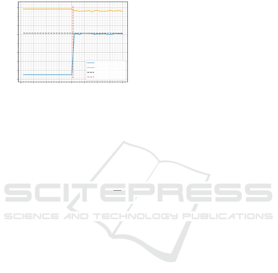
sualized in Figure 6. The figure depicts the develop-
ment of expected profits E
t
over time when utilizing
the Assurance procedure. We used prices = prices
20
with Underbid as B’s underlying strategy and T
i
= 20
time steps for initial exploration.
As discussed in Section 4.2, A will be able to find
the optimal strategy because B’s strategy is determin-
istic and T
i
≥ |prices|. This can be seen clearly in
Figure 6. During exploration with Assurance, A’s ex-
pected profits are mediocre but after exploration, the
expected profits are equal to the optimal profits. In
order to compare the two procedures over a longer
ICORES 2021 - 10th International Conference on Operations Research and Enterprise Systems
66
0 5 10 15 20 25 30 35 40
Time
0.75
1.00
1.25
1.50
1.75
2.00
2.25
2.50
2.75
Profit per Time Step
A’s Profit
B’s Profit
A’s Optimal Profit
Exploration
Figure 6: Profit per time step against Underbid on 20 prices
with with Assurance exploration and T
i
= 20.
time period, we set A’s cumulative profit in propor-
tion to the cumulative profit under the optimal strat-
egy. A’s cumulative profit will be denoted CE
t
and the
cumulative profit under the optimal strategy will be
denoted CO
t
. Consequently, we have CE
t
=
∑
t
i=1
E
i
and CO
t
=
∑
t
i=1
O = t · O. If CE
t
= CO
t
, A found the
optimal strategy or another one that achieves equal
profits. Furthermore, in order for the cumulative prof-
its to be approximately equal, the strategy needs to
be used for several time steps to account for inferior
strategies applied in the past. We will call
CE
t
CO
t
the
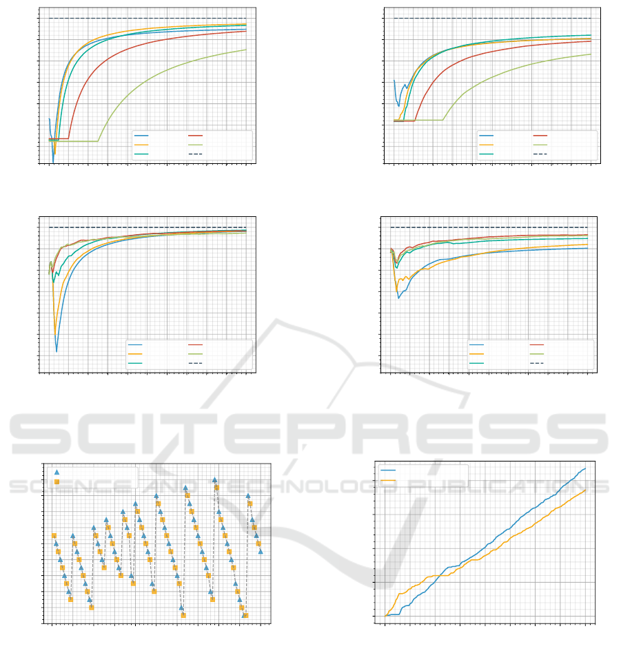
profit ratio. Figure 7 depicts the profit ratio of the As-
surance and Incentive procedure with their respective
configurations for 400 time steps.
Assurance and Underbid Strategy (Figure 7a).
The figure shows that it takes a long time for larger T
i
to account for losses during exploration as we know
that A would find the optimal strategy after T
i
= 20
time steps. T
i
= 10 seems to have found the optimal
strategy after initial losses as well. This can be seen
because the plot is approached by T
i
= 20. These two
configurations as well as T
i
= 40 and T
i
= 100 will
approach the optimal profit ratio of 1 on the infinite
event horizon. With T
i
= 0 the model was not able to
find the optimal strategy which explains why its plot
is being overtaken by that of T
i
= 20.
Assurance and Stochastic Strategy (Figure 7b).
The figure shows that for a stochastic strategy more
exploration is needed. The configuration T
i
= 0 and
T
i
= 10 converge to the same point, which means that
the additional exploration did not contain any bene-
ficial information. T
i
= 20 results in a higher profit
ratio but similar to the deterministic scenario, it takes
very long for larger T
i
to account for missed profits
during the exploration phase.
Incentive and Underbid Strategy (Figure 7c). In
the figure we can see that every configuration after
some initial profits experiences a drop in profit ra-
tio. The reason for that is because the model tries
out less profitable prices after gaining enough infor-
mation about profitable prices.
This is visualized in Figure 8 for λ = 1. The model
continuously tries out higher prices. For a lower λ
proposing these prices happens very fast. That is the
reason why the drop for lower λ is greater compared
to larger λ. Model configurations with larger λ take
longer to gain confidence for the profitable prices be-
fore trying out less profitable prices. This also means
that larger λ take longer to accept that the opponent
strategy is deterministic. It is therefore not surprising
that the order of profit ratio at t = 400 is the ascending
order of λ. Every configuration is able to find the op-
timal strategy. However, we see that the larger λ the
longer it takes for the model to be certain.
Incentive and Stochastic (Figure 7d). The plots in
this figure have a similar shape compared to the same
procedure with Underbid as the underlying opponent
strategy. The drop is less significant which should be
due to the Stochastic being a more forgiving strategy
compared to Underbid. λ = 0.001 seems to not have
received enough opponent reactions which can be
seen as the plot is stagnating for larger t. Moreover,
larger λ perform equally well.
Comparing the results, we decide that the Incentive
procedure should be preferred over the Assurance
procedure for exploration. The Incentive procedure
produces higher profit ratio compared to Assurance
procedure. This is because the later needs exploration
for T
i
≥ |prices| time steps in order to produce a good
strategy which can be clearly seen in the scenario of
the Stochastic strategy. However, if T
i
is too large it
takes very long to compensate the exploration phase.
For the Incentive procedure λ ≈ 1 seems to be ideal.
Moreover, configurations with large λ take too long to
be confident about the opponent’s strategy while con-
figurations with small λ are considerably less likely to
propose a price multiple times.
5.3 Results for Self-adaptive Strategies
The evaluation of the interaction between two self
adapting strategies will be divided into three major
parts. The first of those runs the competition with two
identically configured models and observes how the
competition affects each of these. The second part
focuses on the parameter α and its effect on model’s
performance. The final part examines whether both
Pricing Competition in a Duopoly with Self-adapting Strategies
67
1 40 80 120 160 200 240 280 320 360 400
Time
0.4
0.5
0.6
0.7
0.8
0.9
1.0
Profit Ratio
T
i
= 0
T
i
= 10
T
i
= 20
T
i
= 40
T
i
= 100
Optimal Profit
(a) Assurance exploration against Underbid
1 40 80 120 160 200 240 280 320 360 400
Time
0.4
0.5
0.6
0.7
0.8
0.9
1.0
Profit Ratio
T
i
= 0
T
i
= 10
T
i
= 20
T
i
= 40
T
i
= 100
Optimal Profit
(b) Assurance exploration against Stochastic
1 40 80 120 160 200 240 280 320 360 400
Time
0.4
0.5
0.6
0.7
0.8
0.9
1.0
Profit Ratio
λ = 0.001
λ = 0.5
λ = 1.0
λ = 2.0
λ = 5.0
Optimal Profit
(c) Incentive exploration against Underbid
1 40 80 120 160 200 240 280 320 360 400
Time
0.4
0.5
0.6
0.7
0.8
0.9
1.0
Profit Ratio
λ = 0.001
λ = 0.5
λ = 1.0
λ = 2.0
λ = 5.0
Optimal Profit
(d) Incentive exploration against Stochastic
Figure 7: Profit ratios for Assurance and Incentive exploration against Underbid and Stochastic over 400 time steps.
0 5 10 15 20 25 30 35 40 45 50
Time
0
2
4
6
8
10
12
14
16
18
20
Price
Participant A’s Prices
Participant B’s Prices
Figure 8: Market simulation of the Incentive procedure with
λ = 1 competing against Underbid on 20 prices.
strategies can form a cartel. For all of these tests, we
use an interval split h = 0.5, a discount factor δ = 0.99
and an evaluation time horizon T = 50. Strategy up-
dates are performed frequently with T
d
= 10 in order
to shorten the initial exploration phase. We simulate
each configuration for 2000 time points to account for
long term effects. Additionally, the models use the In-
centive technique, presented in Section 4.2, to explore
prices the competitor has not reacted to.
0 250 500 750 1000 1250 1500 1750 2000
Time
0
1000
2000
3000
4000
Profit
Participant A’s Profit
Participant B’s Profit
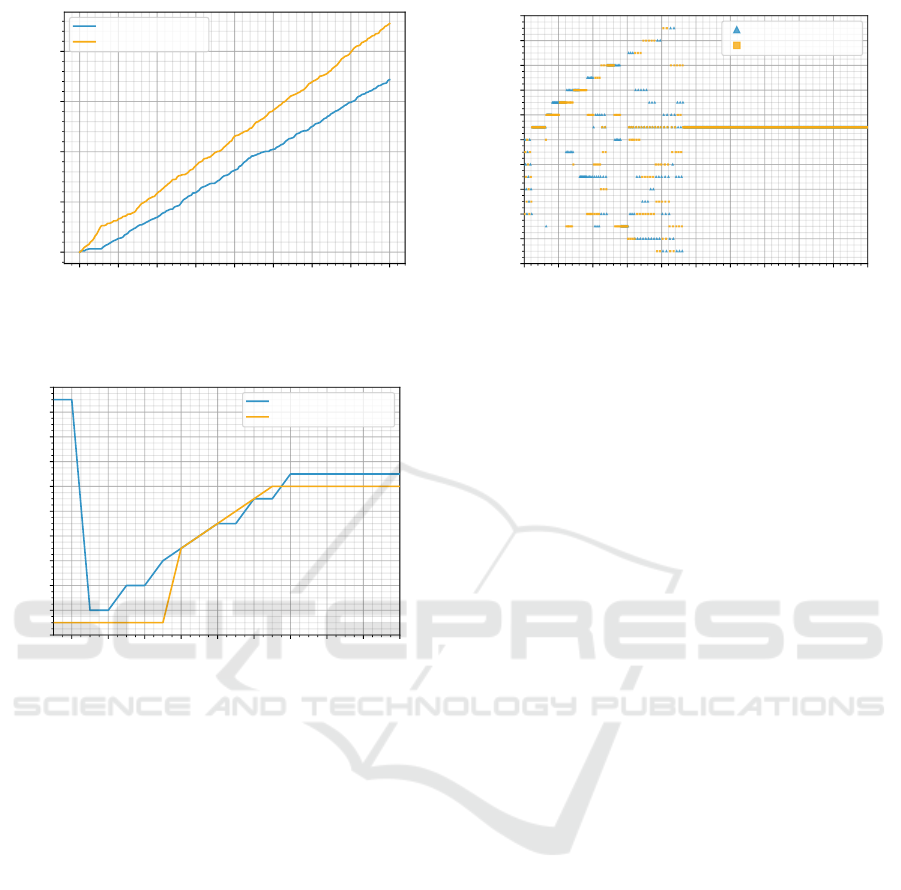
Figure 9: Profit progression of two competing, self-
adapting price strategies.
Identical Start Conditions. In this scenario, we let
two identically configured models compete. Both
models differentiate between new and old reactions,
α 6= 1. We identified α = 0.8 as suitable to account
for focusing on newer reactions while keeping track
of old ones, too. Figure 9 shows the progress of the
profits of both strategies. In the beginning, market
participant B is ahead due to the fact that the strategy
of market participant B has one period of additional
data during the strategy reevaluation. Therefore, it
can finish its exploration phase earlier. However, the
ICORES 2021 - 10th International Conference on Operations Research and Enterprise Systems
68
2 4 6 8 10 12 14 16 18 20
Competitor Price
0
2
4
6
8
10
12
14
16
18
20
Reaction
Participant A’s Strategy
Participant B’s Strategy
(a) Both strategies at t = 100
2 4 6 8 10 12 14 16 18 20
Competitor Price
0
2
4
6
8
10
12
14
16
18
20
Reaction
Participant A’s Strategy
Participant B’s Strategy
(b) Both strategies at t = 400
2 4 6 8 10 12 14 16 18 20
Competitor Price
0
2
4
6
8
10
12
14
16
18
20
Reaction
Participant A’s Strategy
Participant B’s Strategy
(c) Both strategies at t = 1000
Figure 10: Progression of both strategies at different time points t.
earlier update has its disadvantages, too. Market par-
ticipant B notices first that they have to restore a low
price level at some point to gain higher profits in the
future. However, in this scenario market participant
A can exploit this behavior by choosing a low price,
so participant B has to increase the price level. There-
fore, market participant A never has to increase the
price level itself, but can force market participant B
to do so once the price level drops too low. Accord-
ingly, market participant A wins out at some point and
never looses the profit lead again. We see that market
participant B is not able to stop the downward trend
once it started. When competing for an extended pe-
riod of time, both strategies enter a loop of chosen
prices, which both models profit from. While mar-
ket participant B looses the competition, its strategy
is still optimal from its point of view. The alternative
of matching a low price of market participant A is not
lucrative, as there is no guarantee that market partici-
pant A will restore the price level and market partici-
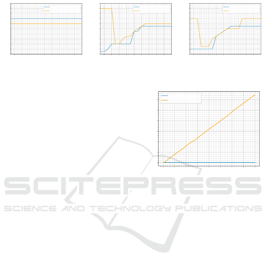
pant B looses profit in the long run. When looking at
the strategy evolution, we see that both models start
with similar strategies to explore the respective com-
petitor’s strategy. Figure 10a shows that market par-
ticipant B is ahead during the exploration phase. Both
strategies evaluate the competitor reactions from most
profitable to least profitable. As we can see, partici-
pant B is already using price 12, while participant A
is still evaluating the more profitable price of 14.
Figure 10b shows the learning progress of both
strategies at t = 400. Market participant B has learned
that it has to restore the price level at some point,
while market participant A exploits B’s strategy by
matching lower prices in order to force B to raise the
price level afterwards. After 1000 time periods, both
strategies do not change any more. The final strate-
gies are presented in Figure 10c. We can see that both
strategies underbid each other in the mid price ranges.
However, they differ in their behavior once the price
drops too low and also in their price reaction on too
high market prices. Moreover, market participant A
0 250 500 750 1000 1250 1500 1750 2000
Time
0
1000
2000
3000
4000
5000
6000
Profit
Participant A’s Profit
Participant B’s Profit
Figure 11: Profit progression of two competing, self-
adapting price strategies with α
A
= 0 and α
B
= 1.
already deems prices below 7 as too low, while mar-
ket participant B only deems below 3 as too low.
α
α
α Deviations. While the previous section focused
on α = 0.8, this section investigates the impact of se-
lected α values on the models’ performances. Fig-
ure 11 shows the competition of two extreme α val-
ues (i.e., α
A
= 0 and α
B
= 1). We see that participant
B wins the competition very decidedly. α = 0 is ob-
served to be the worst possible setting as the incentive
based learning has to start over and over again. This
is due to the fact that the model loses every recorded
price reaction after each strategy evaluation. There-
fore, previously played prices appear to be new to the
unsuspecting model. In the short term, this strategy
can work out because it focuses on high profit prices
first and the model with α = 1 wants to learn about
all prices instead. However, this effect is mitigated as
participant B updates its strategy earlier.
Therefore, we present a more competitive setting
where participant A uses α = 1 and participant B uses
α = 0.5. An α value of 0.5 allows a model to focus on
newer reactions, yet not loosing information on older
ones. Figure 12 shows the profits of both competing
strategies over time. We can see that participant B’s
Pricing Competition in a Duopoly with Self-adapting Strategies
69
0 250 500 750 1000 1250 1500 1750 2000
Time
0
1000
2000
3000
4000
Profit
Participant A’s Profit
Participant B’s Profit
Figure 12: Profit progression of two competing, self-
adapting price strategies with α
A
= 1 and α
B
= 0.5.
2 4 6 8 10 12 14 16 18 20
Competitor Price
0
2
4
6
8
10
12
14
16
18
20
Reaction
Participant A’s Strategy
Participant B’s Strategy
Figure 13: Strategy comparison at t = 1000 with α
A
= 1
and α
B
= 0.5.
strategy using α = 0.5 is more effective.
As we saw earlier, participant B is at a structural
disadvantage. Nonetheless, B is able to win over par-
ticipant A due to the superior α value. In contrast to
the first experiment, participant B is able to force A to
restore the price level, as we can see in Figure 13. Par-
ticipant A is not able to remove misleading reactions
from the early exploration. Thus, market participant A
is not able to compete with market participant B who
adapts its strategy accordingly.
5.4 Results for Cartel Formations
The following focuses on a cartel formation using two
self-learning strategies. While the previous experi-
ments showed that the two models do not form a car-
tel on their own, the introduction of an artificial price
reaction as discussed in Section 4.3 helps with that.
Figure 14 shows the product prices p
A
and p
B
of both
market participants over time.
We observe that both strategies explore the pos-
sible prices at first, as we see a lot of different prices
0 50 100 150 200 250 300 350 400 450 500
Time
0
2
4
6
8
10
12
14
16
18
20
Price
Participant A’s Prices
Participant B’s Prices
Figure 14: Price history with market participant A’s artifi-
cial cartel price reaction.
played. Both participants choose the cartel price some
time, but they do not form a cartel instantly. Given
that participant A will always react to a price p
B
=
p
B
∗ = 11 with p
A
= p
A
∗ = 11, we see that partici-
pant B at some point t ≈ 250 decides to consistently
react to p
A
∗ with p
B
∗ in order to form a cartel. Af-
ter the formation phase, both parties continue to stick
with the cartel price. As expected, the earned profits
of both participants are high and both strategies out-
perform their competing counterparts.
6 CONCLUSION
In recent times, market participants try to adapt their
prices more frequently to gain a competitive edge.
Online markets offer optimal conditions to employ
dynamic pricing strategies, as it is easy to observe
competitor’s prices and to change the own price. We
analyze optimized pricing strategies for different sce-
narios. In all of these, we compete in a duopoly and
operate under an infinite time horizon. Additionally,
we allow for an arbitrary functional dependency be-
tween the sale probability and the current market sit-
uation consisting of two competitors’ prices.
Firstly, we show how to explore the competitor’s
strategy efficiently while losing a minimum profit.
We try out two different ways of estimating the com-
petitor strategy. On the one hand, we simply cycle
through prices to gain more information about spe-
cific prices. On the other hand, we use an incentive
approach for motivating the model to try out prices
that have not been proposed before. We find that the
incentive approach should be preferred over the other
as profits are considered during exploration.
Secondly, we let our self-learning strategies inter-
act with each other. Both of the strategies estimate the
respective competitor’s strategy and adapt their price
ICORES 2021 - 10th International Conference on Operations Research and Enterprise Systems
70

responses in fixed intervals. We observe that equal
strategies evolve over an extended period of time,
but stop evolving at some point. Afterwards, neither
strategy is changed again. When comparing differ-
ent strategies, we observe that diminished knowledge
of past price reactions outperforms settings without
any as well as those with unlimited backward reaction
tracking. Moreover, we slightly modify one strategy
such that it prefers playing a cartel price. We show
that both strategies stop competing once they discover
the cartel price. Although customers suffer from the
high price, it is the most beneficial scenario for both
market participants due to high profits.
REFERENCES
Adida, E. and Perakis, G. (2010). Dynamic pricing and
inventory control: Uncertainty and competition. Op-
erations Research, 58:289–302.
Bitran, G. and Caldentey, R. (2003). An overview of pricing
models for revenue management. Manufacturing and
Service Operations Management, 5:203–229.
Chen, M. and Chen, Z.-L. (2015). Recent developments in
dynamic pricing research: Multiple products, compe-
tition, and limited demand information. Production
and Operations Management, 24:704–731.
den Boer, A. V. (2015). Dynamic pricing and learning: His-
torical origins, current research, and new directions.
Surveys in Operations Research and Management Sci-
ence, 20:1–18.
Do Chung, B., Li, J., Yao, T., Kwon, C., and Friesz, T. L.
(2011). Demand learning and dynamic pricing under
competition in a state-space framework. IEEE Trans-
actions on Engineering Management, 59:240–249.
Gallego, G. and Hu, M. (2014). Dynamic pricing of perish-
able assets under competition. Management Science,
60:1241–1259.
Gallego, G. and Topaloglu, H. (2019). Revenue Manage-
ment and Pricing Analytics. Springer.
Gallego, G. and Wang, R. (2014). Multiproduct price opti-
mization and competition under the nested logit model
with product-differentiated price sensitivities. Opera-
tions Research, 62:450–461.
Hajji, A., Pellerin, R., L
´
eger, P.-M., Gharbi, A., and Babin,
G. (2012). Dynamic pricing models for erp systems
under network externality. International Journal of
Production Economics, 135:708.
He, Q.-C. and Chen, Y.-J. (2018). Dynamic pricing of
electronic products with consumer reviews. Omega,
80:123–134.
Huang, Y.-S., Hsu, C.-S., and Ho, J.-W. (2014). Dynamic
pricing for fashion goods with partial backlogging. In-
ternational Journal of Production Research, 52:4299–
4314.
Levin, Y., McGill, J., and Nediak, M. (2009). Dy-
namic pricing in the presence of strategic consumers
and oligopolistic competition. Management Science,
55:32–46.
Liu, Q. and Zhang, D. (2013). Dynamic pricing compe-
tition with strategic customers under vertical product
differentiation. Management Science, 59:84–101.
Mart
´
ınez-de Alb
´
eniz, V. and Talluri, K. (2011). Dynamic
price competition with fixed capacities. Management
Science, 57:1078–1093.
McGill, J. and van Ryzin, G. (1999). Revenue management:
Research overview and prospects. Transportation Sci-
ence, 33:233–256.
Noel, M. (2007). Edgeworth price cycles, cost-based pric-
ing, and sticky pricing in retail gasoline markets. The
Review of Economics and Statistics, 89:324–334.
Noel, M. (2012). Edgeworth price cycles and intertempo-
ral price discrimination. Energy Economics - ENERG
ECON, 34.
Phillips, R. L. (2005). Pricing and Revenue Optimization.
Stanford University Press.
Schlosser, R. (2019a). Dynamic pricing under competition
with data-driven price anticipations and endogenous
reference price effects. Journal of Revenue and Pric-
ing Management, 16:451–464.
Schlosser, R. (2019b). Stochastic dynamic pricing
with strategic customers and reference price effects.
ICORES 2019, pages 179–188.
Schlosser, R. and Boissier, M. (2017). Optimal price re-
action strategies in the presence of active and passive
competitors. ICORES 2017, pages 47–56.
Schlosser, R. and Boissier, M. (2018). Dynamic pricing
under competition on online marketplaces: A data-
driven approach. International Conference on Knowl-
edge Discovery and Data Mining, pages 705–714.
Schlosser, R. and Richly, K. (2018). Dynamic pricing
strategies in a finite horizon duopoly with partial in-
formation. ICORES 2018, pages 21–30.
Sweeting, A. (2012). Dynamic pricing behavior in perish-
able goods markets: Evidence from secondary mar-
kets for major league baseball tickets. Journal of Po-
litical Economy, 120:1133–1172.
Talluri, K. T. and Van Ryzin, G. J. (2006). The Theory and
Practice of Revenue Management. Springer.
Tong, T., Dai, H., Xiao, Q., and Yan, N. (2020). Will dy-
namic pricing outperform? theoretical analysis and
empirical evidence from o2o on-demand food service
market. International Journal of Production Eco-
nomics, 219:375–385.
Tsai, W.-H. and Hung, S.-J. (2009). Dynamic pricing and
revenue management process in internet retailing un-
der uncertainty: An integrated real options approach.
Omega, 37:471–481.
Pricing Competition in a Duopoly with Self-adapting Strategies
71
