Network Topology Identiﬁcation using Supervised Pattern Recognition

Neural Networks

Aniruddha Perumalla

, Ahmet Taha Koru

and Eric Norman Johnson

Department of Aerospace Engineering, Pennsylvania State University, University Park, PA, U.S.A.

Keywords:

Multi-Agent Systems, Neural Networks, Topology Identiﬁcation, Machine Learning, Counterintelligence,

Countersurveillance, Autonomous Systems, Graph Theory, Linear Consensus, Pattern Recognition,

Supervised Learning.

Abstract:

This paper studies the network topology identiﬁcation of multi-agent systems with single-integrator dynamics

using supervised pattern recognition networks. We split the problem into two classes: (i) small-scale systems,

and (ii) large-scale systems. In the small-scale case, we generate all connected (undirected) graphs. A ﬁnite

family of vectors represent all possible initial conditions by gridding the interval 0 and 1 for each agent.

The system responses for all graphs with all initial conditions are the training data for the supervised pattern

recognition neural network. This network is successful in identiﬁcation of the most connected node in up

to nearly 99% of cases involving small-scale systems. We present the accuracy of the trained network for

network topology identiﬁcation with respect to grid space. Then, an algorithm predicated on the pattern

recognition network, which is trained for a small-scale system, identiﬁes the most connected node in large-

scale systems. Monte Carlo simulations estimate the accuracy of the algorithm. We also present the results for

these simulations, which demonstrate that the algorithm succeeds in ﬁnding the most connected node in more

than 60% of the test cases.

1 INTRODUCTION

The theoretical advances in cooperative control of

multi-agent systems lead swarm systems to take place

in engineering applications. Autonomous transporta-

tion (Teodorovic, 2003), complex power networks

(Bidram et al., 2014), water distribution (de Roo et al.,

2015), multi-robot systems (Ota, 2006), and modern

warfare (Scharre, 2018) are among the examples. In-

telligent group behaviors emerge from the swarming

of a group of individuals with poor abilities (Tan and

Zheng, 2013). Therefore, swarming fulﬁlls the de-

mand to accomplish complex tasks.

The agents of a swarm share their sensor measure-

ments through a communication network to cooper-

ate. However, the network topology is not directly

available in some applications, for instance the in-

teractions between brain neurons (Vald

es-Sosa et al.,

2005) and gene regulatory networks in biological sys-

tems (Julius et al., 2009). Another interesting exam-

ple is the case of counter-swarm systems. Such a sys-

https://orcid.org/0000-0002-2618-7032

https://orcid.org/0000-0001-8191-2324

tem may require the knowledge of the opponent net-

work topology to efﬁciently neutralize.

Although it is a system identiﬁcation application;

yet, conventional methods may fail to identify some

network topologies (see the discussion in subsection

2.3). Consequently, the network topology identiﬁca-

tion studies draw attention of researchers. The authors

of (Gonc¸alves and Warnick, 2008) study the network

topology identiﬁcation of linear time-invariant sys-

tems. A node-knockout procedure identify the topol-

ogy in consensus-type network (Nabi-Abdolyouseﬁ

and Mesbahi, 2012). Reference (Rahimian et al.,

2013) discusses the identiﬁability of links and nodes

of multi-agent systems under the agreement proto-

col. Stochastic perturbations recover the underlying

topologies of noise-contaminated complex dynamical

networks (Wu et al., 2015). The authors of (Sun and

Dai, 2015) reformulate the network topology iden-

tiﬁcation problem as a quadratic optimization prob-

lem. The constrained Lyapunov equations establish

network reconstruction algorithms (van Waarde et al.,

2019).

In this paper, we utilize neural networks to iden-

tify an unknown network topology. We consider the

258

Perumalla, A., Koru, A. and Johnson, E.

Network Topology Identiﬁcation using Supervised Pattern Recognition Neural Networks.

DOI: 10.5220/0010231902580264

In Proceedings of the 13th International Conference on Agents and Artiﬁcial Intelligence (ICAART 2021) - Volume 1, pages 258-264

ISBN: 978-989-758-484-8

single-integrator dynamics with a consensus protocol

over a ﬁxed connected (undirected) graph. We split

the problem into two: (i) identiﬁcation of the entire

graph for small-scale systems, and (ii) identiﬁcation

of the most connected node for large-scale systems.

For problem (i), we trained a pattern recognition neu-

ral network to identify the topology of a four-node

network using simulated data of the observed state

of the network over a small period of time. We pro-

pose an algorithm predicated on the neural networks

trained in a small-scale setup to reveal the most con-

nected node(s) in a large-scale system.

1.1 Motivation

Countersurveillance is the primary motivator of this

algorithm. If one wishes to attack an opponent swarm

of vehicles, knowledge of the swarm’s network topol-

ogy may signiﬁcantly increase the efﬁciency and ef-

fectiveness of one’s attack. For instance, if it is known

that the topology of the swarm adheres to a spoked-

hub or star/“leader-follower” network structure (visu-

alized in Figure 1, with node 10 being the leader),

focusing the attack on the leader of the swarm may

be sufﬁcient to incapacitate the swarm. In general,

knowledge of the opponent network topology allows

a valuable additional basis on which countersurveil-

lance measures may weigh the importance of speciﬁc

members of the opponent system and thereafter dis-

tribute their resources more effectively.

Figure 1: An example leader-follower network topology.

2 PRELIMINARIES

2.1 Notation

The notation of this paper is standard. Speciﬁcally,

R, R

, R

n×m

, Z

respectively stand for the sets of

all real numbers, n-dimensional real column vectors,

n×m real matrices, and positive integers. The symbol

“,” denotes equality by deﬁnition. We also write I

for the n×n identity matrix, 0

n×m

for the n×m matrix

with zero entries, 1

for the n × 1 vector of all ones,

⊗ for Kronecker product. The symbol P (X) denotes

the power set and |X| denotes cardinality of a set X.

2.2 Graph Theory

Consider a ﬁxed (i.e. time-invariant) directed or undi-

rected graph (representing network topology) G =

{V ,E}, where V = {v

,..., v

} is a non-empty

ﬁnite set of N nodes and E ⊆ V × V is a set of edges.

There is an edge rooted at node v

and ended at v

(i.e. (v

) ∈ E) if and only if v

receives informa-

tion from v

. A(G) = [a

i j

] ∈ {0,1}

N×N

denotes the

adjacency matrix. We only consider boolean graphs;

that is, a

i j

= 1 ⇔ (v

) ∈ E and a

i j

= 0 otherwise.

Furthermore, repeated edges and self-loops are not al-

lowed; that is, a

= 0, ∀i ∈ I

. If (v

) ∈ E, then

the nodes i and j are neighbours. The set of neigh-

bors of node v

is denoted as N

= { j | (v

) ∈ E}.

A graph with the property that a

i j

= a

is undirected.

The in-degree matrix is deﬁned by D(G) = diag(d

)

with d

∑

j∈N

i j

. A directed path from node v

node v

is a sequence of successive edges in the form

{(v

),(v

),.. ., (v

)}. The Laplacian of the

graph G is deﬁned as L(G) = D(G) − A(G). A con-

nected graph is an undirected graph which has at least

one vertex and between every pair of vertices of which

there is a path.

2.3 Agreement Protocol

Consider the consensus problem of a group of N

agents over a ﬁxed connected network topology G

with the single-integrator dynamics given by

˙x

(t) = u

(t), x

(0) = x

, t ≥ 0, (1)

where x

(t) ∈ R is the state, and u

(t) ∈ R is the input

for each agent i ∈ {1,..., N}. The local control proto-

col for each agent i is given by

(t) =

∑

j∈N

i j

− x

). (2)

We represent the overall closed-loop system in the

compact form as

˙x(t) = −L(G)x(t) (3)

where x(t) , [x

(t),...,x

(t)]

. The solution of (3)

x(t) = e

−L(G)t

x(0). (4)

The local voting protocol in (2) guarantees consensus

of the single-integrator dynamics in (1) if and only

if G has a spanning tree (see Theorem 2.2 in (Lewis

Network Topology Identiﬁcation using Supervised Pattern Recognition Neural Networks

259

1 2

Figure 2: The system in (4) is not identiﬁable from x(0) for

this network topology.

et al., 2014)). It is well-known that each ﬁnite con-

nected graph has at least one spanning tree.

This paper studies the identiﬁcation of L(G) from

a single solution x(t). This identiﬁcation reveals the

underlying network topology G. However, conven-

tional methods may fail to identify L(G) from (4). A

Laplacian matrix L(G) is identiﬁable with (3) from

x(0) if and only if the matrix given by

R(G) ,



I − L(G) (−L(G))

... (−L(G))

N−1



x(0) (5)

is full rank for all L(G) in an open set (see Theorem

2.5 in (Stanhope et al., 2014)). Consider any initial

condition x(0) = [x

, x

]

∈ R

and the net-

work topology G

seen in Figure 2 where

L(G

) =





2 −1 −1

−1 2 −1

−1 −1 2





(6)

For this particular network topology,

R(G

) =





− 2x

+ x

− 3x

− 2x

+ x

− 3x

+ x

− 2x

− 3x





(7)

and rank(R(G

)) = 2. The system in (3) with L(G

)

faces collinearity problems in least squares estimation

for any initial condition x(0) ∈ R

To overcome this, we train a supervised pat-

tern recognition neural network to identify a network

topology. Thus, we avoid identifying L in R

N×N

. In-

stead, the trained neural network distinguishes L(G)

in the set of all possible N−dimensional communica-

tion network topologies.

3 SMALL-SCALE SYSTEMS

We deﬁne systems with less than or equal to ﬁve

nodes (i.e., N ≤ 5) as small-scale systems. The rea-

son is that the number of connected undirected graphs

grows dramatically as N increases

. Due to limita-

tions in training data memory and network training

time brought on by this dramatic increase, efﬁcient

The integer sequence A001187 in the On-Line En-

cyclopedia of Integer Sequences presents the number of

connected undirected graphs (i.e., the length of G

list

) for

N ∈ {0,1,2,...}.

p,q

L(G)

Hidden

layer

Input:

Observed

Dynamics

Output:

Graph

Pattern

Identiﬁer

Identiﬁed

Graph

Figure 3: Illustration of the proposed pattern recognition

network for small-scale system network topology identiﬁ-

cation.

training is not manageable when N > 5. Although it is

possible for the network training dataset to be expan-

sive enough to cover at most 728 such graphs when

N ≤ 5 (e.g., our training dataset for a 4-node system

occupied roughly 20 MB), it is expensive in terms of

both memory and training time to construct a train-

ing dataset that sufﬁciently captures the dynamics of

cases involving all such graphs when N = 6 (26 704),

N = 7 (1 866 256), or greater.

The purpose of the neural network is to identify

the graph G, which is illustrated in Fig 3. Thus, x(t)

is the input and G is the output of the neural network

system. We train the neural network with solutions in

(4) covering as many as possible scenarios. To this

end, we use all of the connected undirected graphs

with degree N. Instead of considering all R

, we fo-

cus on [0,1]

to get samples from all possible initial

conditions x(0). Any solution in (4) can be scaled and

translated such that x(0) ∈ [0,1]

. We present the de-

tails throughout this section.

3.1 The Training Data Set

3.1.1 Generating All Connected Undirected

Graphs

For N number of nodes, there are

(

)

many possi-

ble undirected graphs; we generate all of them. An

undirected graph is connected if and only if the rank

of the corresponding Laplacian matrix is N − 1 (see

Remark 4 in (Olfati-Saber and Murray, 2004)). Us-

ing this theorem, we choose the connected undirected

graphs with degree N among all of the possible graphs

with degree N and store them in a set G

list

ICAART 2021 - 13th International Conference on Agents and Artiﬁcial Intelligence

260

3.1.2 Generating Initial Conditions

The set x

samples

, {k/K | k ∈ {0, .. .,K}, K ∈ Z

}

contains real numbers 0, 1/K, 2/K,. .. , 1 where 1/K

represents the grid spacing. We generate initial con-

ditions x(0) using the elements in x

samples

such that

= 0, x

= 1, x

∈ x

samples

, and

≤ x

≤ ·· · ≤ x

. (8)

For instance, [0, 0,1]

, [0,0.5,1]

, and [0,1, 1]

are

the initial conditions for N = 3 and K = 2. We store

the initial conditions in a set x

0,list

Note that any initial condition x(0) ∈ R

is con-

sistent with (8) after proper relabeling of the nodes.

Therefore, this method avoids the redundant solutions

and decreases the memory requirements.

3.1.3 Generating the Training Dataset

Let ∆t > 0 be the chosen sampling period (timestep

length), n

be the number of samples. The product of

and ∆t forms the total duration of the simulated dy-

namics. Let also e

be the N-dimensional vector of all

zeros except its p

entry. e

serves as an “identiﬁer”

for the p

graph. For all G

∈ G

list

and x

∈ x

0,list

, the

inputs

p,q

, e

−L(G

)∆t

,..., e

−L(G

∆t

(9)

and the outputs Y

p,q

, e

construct the training

data set D = {(X

p,q

) | p = 1,.. ., |G

list

|, q =

1,..., |x

0,list

|}. We trained the supervised pattern

recognition neural networks using all input-output

data in D using MATLAB.

3.2 Validation

We train the network with the initial condition sam-

ples which belong to set [0, 1]

. However, the initial

condition belongs to R

in general. The following

lemma is useful to scale and translate any solution (4)

to modify its initial condition to be consistent with

training data.

Lemma 1. For any graph G, x(t) = e

−L(G)t

x(0)

if and only if S(x(t)+ T 1

) = e

−L(G)t

S(x(0) + T 1

)

where S 6= 0 and S, T ∈ R.

Proof. The matrix exponential is the power series as

−L(G)t

= I +

∞

∑

k=1

−L

(G)t

(10)

by deﬁnition. As per graph theory, L(G)1

= 0

since 1

is the right eigenvector corresponding to the

eigenvalue 0 of L(G) (Lewis et al., 2014). Thus,

−L(G)t

= 1

from (10). The rest of the proof is

algebraic manipulations.

Consider that we observe the outputs ¯x

(t) of a

multi-agent system with an underlying communica-

tion topology G

. We assume ¯x

(0) ≤ ·· · ≤ ¯x

(0)

without loss of generality. Otherwise, we can relabel

the nodes to satisfy this constraint. Let the observa-

tion matrix be

X = [ ¯x(0), ¯x(∆t),. .. , ¯x(n

∆t)], (11)

S = max

¯x

(0) − min

¯x

(0), and T = −min

¯x

(0).

Note that x(0) ∈ [0,1]

where x(t) = S(¯x(t) + T 1

Thus, X = S(

X + T (1

⊗ 1

)) is an appropriate ob-

servation matrix to identify G

using trained pattern

recognition network. The underlying graph is same

for both X and

X from Lemma 1. Thus, the output of

the pattern recognition neural network is L(G

4 LARGE-SCALE SYSTEMS

We deﬁne systems with more than ﬁve nodes, N > 5,

as large-scale systems. In this case, we present an al-

gorithm to detect the most connected node (“primary”

node) of a communication network topology. To this

end, we use a pattern recognition network which is

trained for a small-scale system.

4.1 Determining the Most-connected

Node of Large-scale Systems

Consider the outputs

(t) of a large-scale multi-agent

system. The following algorithm aims to reveal the

most connected node of its communication network

topology.

Step 0: This step contains ofﬂine training and com-

putations which are performed once and stored.

Step 0.1: Set K > 0 and 3 ≤ N

≤ 5. Generate all con-

nected undirected graphs G

list

, generate initial condi-

tion samples list x

0,list

with N

and K, and generate the

data set D (see Section 3). Train the pattern recogni-

tion network using D.

Step 0.2: Let I

, {1, 2,. ..,N}. Compute all N

combinations of I

, C = {C

∈ P (I

) | |C

| = N

Step 1: Set the number of links α

= 0, i = 1,. .. ,N.

Step 2: Iterate for all C

∈ C where r = 1, .. ., |C|.

Step 2.1: Let

, I

\ C

, and x

(t) ,

∑

i∈

(t).

Compute ¯x

(t) , (N

(t) + x

(t))/N, i ∈ C

Network Topology Identiﬁcation using Supervised Pattern Recognition Neural Networks

261

Step 2.2: Consider the observation of ¯x

(t) from a

small-scale system with degree N

. Construct the ob-

servation matrix X by reordering, scaling and trans-

lating the set of ¯x

(t) (see Subsection 3.2).

Step 2.3: Identify L(G) using the trained pattern

recognition network. Increment the corresponding

number of links α

using L(G).

Step 3: The most connected node is the one owning

the largest number of links arg max

5 RESULTS

Some aspects of our testing procedure remained the

same for both small-scale and large-scale systems.

Training of the pattern recognition neural network in

each case was done through the patternnet function

in MATLAB’s Deep Learning toolbox (The Math-

Works, Inc., 2019), with a single hidden layer and

otherwise default arguments. The size of this hidden

layer was varied from 5 to 75 to view its effect on ac-

curacy of the small-scale systems, but was set to 50

for the large-scale systems. In the small-scale system,

in which generation of all possible graphs G

list

for

training and testing purposes was possible due to its

small length

, population of G

list

was done ourselves.

In the large-scale system application for N ∈ {7,8,9},

the training with graphs from G

list

was accomplished

similarly. However, generation of G

list

for large-scale

systems imposes a high computational load and there-

fore requires a long duration. We avoid this require-

ment by rather drawing a small random sample G

size n from G

list

for the testing of the large-scale sys-

tems. For this sampling, we utilize nauty (McKay

and Piperno, 2013), a tool that can quickly gener-

ate graphs; in particular, we make use of nauty’s

genrang program.

5.1 Small-scale Systems

Several pattern-recognition networks were trained to

predict the exact network topology of the small-scale

systems. We varied the size of the training dataset

by manipulating K, since K inﬂuences the length of

0,list

, which corresponds to the number of initial con-

ditions generated. As K increases, the number of

combinations of initial conditions and graphs used to

generate the training data grows. In addition, as pre-

viously mentioned, we varied the size of the hidden

layer to check its impact on the accuracy of the pre-

dictions. We tested the trained pattern recognition

See the aforementioned A001187.

network using a dataset assembled similarly to the

training data, but whose initial conditions were not

restricted to the “sample” space x

sample

. The results

of the testing for each combination of K and hidden

layer size are presented in Table 1.

Table 1: Identiﬁcation accuracy for G

with respect to var-

ious K and size of the hidden layer.

Size of the Hidden Layer

5 25 50 75

5 31.08% 65.59% 78.96% 95.05%

10 61.36% 98.26% 96.78% 94.31%

15 97.53% 98.76% 98.51% 97.03%

20 97.61% 98.76% 97.05$ 99.19%

The network becomes more accurate as the number

of initial conditions used for training grows; we ex-

pect this trend, as the discrepancy of the network’s

initial condition space decreases with increasing K.

A similar trend is observed for the increase in hidden

layer size. However, it is appropriate to be wary of

the tradeoff between high network accuracy and both

overﬁtting as the size of the hidden layer grows and

higher memory requirements as K grows.

As an aside, it should be noted again that the dis-

tinction between small-scale and large-scale systems

is largely motivated by neural network training time.

As an example: a network trained for a 4-node system

with K = 10 and 5 hidden layers required just 52 sec-

onds for training, whereas a network trained with the

same conﬁguration for a 5-node system required 172

minutes for training, so the increase in training time

is quite signiﬁcant.

5.2 Large-scale Systems

Using the process put forth in Section 3.2, we trained

a pattern-recognition network using initial condition

samples belonging to [0,1]

(i.e., data from a 4-node

small-scale system). Thereafter, through the follow-

ing method we generated a testing dataset through

which this small-scale-trained network was used to

predict the primary and secondary nodes of a system

with N = 7. A set of ﬁve initial conditions x

for

N = 7 was ﬁrst generated using the method outlined in

Section 3. A subset G

of size n was drawn from G

list

through nauty. For every combination (i, j) of initial

condition x

,i ∈ {1, ...,5} and graph G

, j ∈ {1,...,n},

the test inputs X were generated through Equation

9. The algorithm described in Section 4.1 was then

used to identify the most connected (primary), as well

as the second-most-connected (secondary), nodes for

each combination (i, j) making up the test dataset.

ICAART 2021 - 13th International Conference on Agents and Artiﬁcial Intelligence

262

The primary “success” of the algorithm for a given

graph sample size n was deﬁned as the percentage of

correct primary node identiﬁcation across all combi-

nations (i, j); the secondary success was deﬁned simi-

larly. This entire testing process was repeated 3 times

for each sample size n ∈ {10, 20,..., 250} and the av-

erage success was taken to be the mean of the primary

success over the 3 repetitions for each sample size.

100

130

160

190

220

250

280

310

340

370

400

Number of Graphs Sampled

Mean Success (%)

Mean Success of 4-Node Trained Network for

Prediction of Primary and Secondary Nodes

of 7-Node Graph

Primary Node

Secondary Node

Figure 4: Results of testing a pattern-recognition network

trained on data from a small-scale (4-node) system on large-

scale (7-node) data.

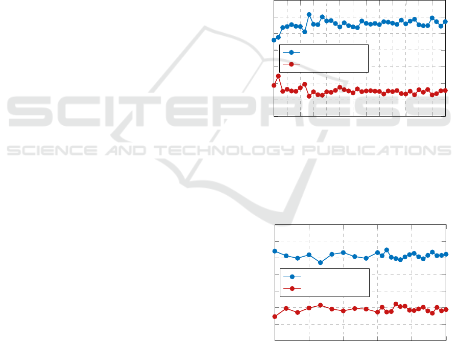
Figure 4 displays the results of the large-scale testing

for N = 7 as the testing dataset grows in size propor-

tionally to n, the number of samples from G

list

. The

network trained on small-scale data is successful in

identiﬁcation of the primary node in roughly 65% of

cases; in addition, it is successful in identiﬁcation of

the secondary node in roughly 25% of the cases.

The same process was also used to test the small-

scale network for primary/secondary node prediction

of large-scale systems of size N ∈ {8, 9}. We include

the visualizations of those results (Figs. 6 and 7),

which yielded similar results to the 7-node test case,

in the appendix.

We also repeated the large-scale testing for the 7-

node conﬁguration with noise in the single-integrator

consensus dynamics included to test the robustness of

our method to uncertainty. Whereas the original con-

ﬁguration assumed “perfect” observation of agent dy-

namics, white Gaussian noise models the uncertainty

in the observations of the positions of each agent,

which would be present in a real countersurveillance

scenario. The results of the simulation including

white Gaussian noise with variances 0.1 and 0.25 in

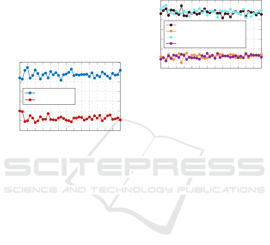
observations of each agent are displayed in Figure 5.

Comparison to Figure 4 indicates that our method is

generally robust to this uncertainty, as the accuracy

100

130

160

190

220

250

280

310

340

370

400

Number of Graphs Sampled

Mean Success (%)

Mean Success of 4-Node Trained Network for

Prediction of Primary and Secondary Nodes

of 7-Node Graph (incl. White Gaussian Noise)

Primary Node (Noise Variance 0.10)

Secondary Node (Noise Variance 0.10)

Primary Node (Noise Variance 0.25)

Secondary Node (Noise Variance 0.25)

Figure 5: Results of testing a pattern-recognition network

trained on data from a small-scale (4-node) system on large-

scale (7-node) data, including white Gaussian noise with

variances 0.1 and 0.25 in the single-integrator consensus

dynamics.

in identiﬁcation of the primary and secondary nodes

does not change signiﬁcantly for either uncertainty

variance examined.

We approximate the convergence of our method

via these simulations. Based on the results of the

Monte Carlo simulations for N ∈ 7,8,9 sampling up

to 400 graphs from the pools, our method is gener-

ally successful in identiﬁcation of the most connected

node in at least 60% of cases for large-scale (N > 5)

systems, even in the presence of uncertainty modelled

as white Gaussian noise. It is also generally suc-

cessful in identiﬁcation of the second-most connected

node in at least 20% of cases.

6 CONCLUSIONS

We found that using our method, the pattern-

recognition network was highly accurate in predicting

the network topology of small-scale systems. Further-

more, such a pattern-recognition network was suc-

cessful in recognizing the most connected nodes of

large-scale systems. Future work may focus on train-

ing the network to recognize network topologies of

systems with different closed-loop dynamics apart

from that of the linear consensus protocol.

Network Topology Identiﬁcation using Supervised Pattern Recognition Neural Networks

263

REFERENCES

Bidram, A., Lewis, F. L., and Davoudi, A. (2014). Dis-

tributed control systems for small-scale power net-

works: Using multiagent cooperative control theory.

IEEE Control Systems Magazine, 34(6):56–77.

de Roo, F. V., Tejada, A., van Waarde, H., and Trentelman,

H. L. (2015). Towards observer-based fault detection

and isolation for branched water distribution networks

without cycles. In 2015 European Control Conference

(ECC), pages 3280–3285. IEEE.

Gonc¸alves, J. and Warnick, S. (2008). Necessary and suf-

ﬁcient conditions for dynamical structure reconstruc-

tion of lti networks. IEEE Transactions on Automatic

Control, 53(7):1670–1674.

Julius, A., Zavlanos, M., Boyd, S., and Pappas, G. J. (2009).

Genetic network identiﬁcation using convex program-

ming. IET systems biology, 3(3):155–166.

Lewis, F. L., Zhang, H., Hengster-Movric, K., and Das, A.

(2014). Cooperative control of multi-agent systems:

Optimal and adaptive design approaches. Springer-

Verlag, London, England.

McKay, B. D. and Piperno, A. (2013). Nauty and traces

user’s guide (version 2.5). Computer Science Depart-

ment, Australian National University, Canberra, Aus-

tralia.

Nabi-Abdolyouseﬁ, M. and Mesbahi, M. (2012). Network

identiﬁcation via node knockout. IEEE Transactions

on Automatic Control, 57(12):3214–3219.

Olfati-Saber, R. and Murray, R. M. (2004). Consensus

problems in networks of agents with switching topol-

ogy and time-delays. IEEE Transactions on automatic

control, 49(9):1520–1533.

Ota, J. (2006). Multi-agent robot systems as distributed au-

tonomous systems. Advanced engineering informat-

ics, 20(1):59–70.

Rahimian, M. A., Ajorlou, A., Tutunov, R., and Aghdam,

A. G. (2013). Identiﬁability of links and nodes in

multi-agent systems under the agreement protocol.

In 2013 American Control Conference, pages 6853–

6858. IEEE.

Scharre, P. (2018). How swarming will change warfare.

Bulletin of the atomic scientists, 74(6):385–389.

Stanhope, S., Rubin, J. E., and Swigon, D. (2014). Identi-

ﬁability of linear and linear-in-parameters dynamical

systems from a single trajectory. SIAM Journal on

Applied Dynamical Systems, 13(4):1792–1815.

Sun, C. and Dai, R. (2015). Identiﬁcation of network topol-

ogy via quadratic optimization. In 2015 American

Control Conference (ACC), pages 5752–5757. IEEE.

Tan, Y. and Zheng, Z. (2013). Research advance in swarm

robotics. Defence Technology, 9(1):18–39.

Teodorovic, D. (2003). Transport modeling by multi-agent

systems: a swarm intelligence approach. Transporta-

tion planning and Technology, 26(4):289–312.

The MathWorks, Inc. (2019). Deep Learning Toolbox,

MATLAB 2019a. Natick, Massachusetts, U.S.

Vald

es-Sosa, P. A., S

anchez-Bornot, J. M., Lage-

Castellanos, A., Vega-Hern

andez, M., Bosch-Bayard,

J., Melie-Garc

ıa, L., and Canales-Rodr

ıguez, E.

(2005). Estimating brain functional connectivity with

sparse multivariate autoregression. Philosophical

Transactions of the Royal Society B: Biological Sci-

ences, 360(1457):969–981.

van Waarde, H. J., Tesi, P., and Camlibel, M. K. (2019).

Topology reconstruction of dynamical networks via

constrained lyapunov equations. IEEE Transactions

on Automatic Control, 64(10):4300–4306.

Wu, X., Zhao, X., L

u, J., Tang, L., and an Lu, J. (2015).

Identifying topologies of complex dynamical net-

works with stochastic perturbations. IEEE Transac-

tions on Control of Network Systems, 3(4):379–389.

APPENDIX

100

130

160

190

220

250

280

310

340

370

400

Number of Graphs Sampled

Mean Success (%)

Mean Success of 4-Node Trained Network for

Prediction of P.-S. Nodes of 8-Node Graph

Primary Node

Secondary Node

Figure 6: Results of testing a pattern-recognition network

trained on data from a small-scale (4-node) system on large-

scale (8-node) data.

100

175 250 325

400

Number of Graphs Sampled

Mean Success (%)

Mean Success of 4-Node Trained Network for

Prediction of P.-S. Nodes of 9-Node Graph

Primary Node

Secondary Node

Figure 7: Results of testing a pattern-recognition network

trained on data from a small-scale (4-node) system on large-

scale (9-node) data.

ICAART 2021 - 13th International Conference on Agents and Artiﬁcial Intelligence

264