
Elliptical Fitting as an Alternative Approach to Complex Nonlinear Least
Squares Regression for Modeling Electrochemical Impedance
Spectroscopy
Norman Pfeiffer
1 a
, Toni Wachter
1
, J
¨
urgen Frickel
2
, Christian Hofmann
1
, Abdelhamid Errachid
3
and
Albert Heuberger
2
1
Fraunhofer IIS, Fraunhofer Institute for Integrated Circuits, Am Wolfsmantel 33, 91058 Erlangen, Germany
2
Lehrstuhl f
¨
ur Informationstechnik mit dem Schwerpunkt Kommunikationselektronik (LIKE),
Friedrich-Alexander Universit
¨
at Erlangen-N
¨
urnberg, Am Wolfsmantel 33, 91058 Erlangen, Germany
3
Institut des Sciences Analytiques, Universit
´
e de Lyon, 5 rue de la Doua, 69100 Villeurbanne, France
Keywords:
Electrochemical Impedance Spectroscopy, Elliptical Fitting, Randles Circuit, Least Squares Fitting, Charge
Transfer Resistance, Complex Nonlinear Least Squares.
Abstract:
Electrochemical impedance spectroscopy is an important procedure with the ability to describe a wide range of
physical and chemical properties of electrochemical systems. The spectral behavior of impedimetric sensors
is mostly described by the Randles circuit, whose parameters are determined by regression techniques on the
basis of measured spectra. The charge transfer resistance as one of these parameters is often used as sensor
response. In the laboratory environment, the regression is usually performed by commercial software, but
for integrated, application-oriented solutions, separate approaches must be pursued. This work presents an
approach for elliptical fitting of the curve in the Nyquist plot, which is compared to the complex nonlinear
least squares (CNLS) regression technique. For this purpose, artificial spectra were generated, which were
considered both with and without noise superposition. Although the average error in calculating the charge
transfer resistance from noisy signals using the elliptical fitting of −2.7% was worse than the CNLS with
2.4 ·10
−2
%, the former required only about
1
/225 of the computing time compared to the latter. Following
application-oriented evaluations of the achievable accuracies, the elliptical approach may turn out to be a
resource saving alternative.
1 INTRODUCTION
Electrochemical impedance spectroscopy (EIS) is a
common measurement technology for the analysis of
biosensors, such as FET-based structures (Kharitonov
et al., 2001). Its advantage is the description of chem-
ical and physical phenomena of an electrochemical
system, thus allows the characterization of the electri-
cal properties of the sensor surface and the investiga-
tion of interfacial reaction mechanisms (Macdonald,
1990). Furthermore, impedimetric biosensors have
other advantages such as label-free measurements,
miniaturization capability, low production costs etc.
(Prodromidis, 2010). In research EIS is used in vari-
ous chemical and medical applications for the analy-
sis of biosensors, e.g. for the diagnosis of heart dis-
a
https://orcid.org/0000-0002-6839-3002
eases (Halima et al., 2019) or of Alzheimer’s disease
(Rushworth et al., 2014), for the detection of bacte-
ria as Escherichia coli or viruses (Leva-Bueno et al.,
2020) or for detection of cancer cells (Chowdhury
et al., 2018).
The application-oriented interpretation of the
impedance spectra of biosensors is usually done by
modeling the biofunctionalized sensor area. For
this purpose an equivalent circuit diagram is ap-
plied, which describes the electrochemical and phys-
ical phenomena. As a model for an electrode in con-
tact with an electrolyte, the so called Randles circuit is
used, which describes a one-step charge transfer pro-
cess involving the diffusion of reactants to the inter-
face (Barsoukov and Macdonald, 2005). In the ma-
jority of published EIS studies, different interface pa-
rameters such as charge transfer resistance R
ct
or dou-
ble layer capacitance C
dl
are determined by modeling
42
Pfeiffer, N., Wachter, T., Frickel, J., Hofmann, C., Errachid, A. and Heuberger, A.
Elliptical Fitting as an Alternative Approach to Complex Nonlinear Least Squares Regression for Modeling Electrochemical Impedance Spectroscopy.
DOI: 10.5220/0010231600420049
In Proceedings of the 14th International Joint Conference on Biomedical Engineering Systems and Technologies (BIOSTEC 2021) - Volume 4: BIOSIGNALS, pages 42-49
ISBN: 978-989-758-490-9
Copyright
c
2021 by SCITEPRESS – Science and Technology Publications, Lda. All rights reserved

(Pejcic and De Marco, 2006). Within the scope of sci-
entific publications, commercial software is usually
used to realize the modeling, which is performed by
a complex nonlinear least squares (CNLS) regression
technique (Kauffman, 2009) with the electrical equiv-
alent circuit diagram. Alternatively, R
ct
is determined
manually at the second extrapolated intersection with
the real axis on the low-frequency side of the Nyquist
plot, thus by a geometric approach. This method for
estimating R
ct
is used extensively in the electrochem-
ical field (Randviir and Banks, 2013).
Electrochemical biosensors can be used in a vari-
ety of applications, such as the examination of sweat,
saliva, blood or urine as part of a wearable sensor
(Sun et al., 2016) (Dang et al., 2018) (Sgobbi et al.,
2016). Apart from medical applications, also small
and energy-efficient devices for gas monitoring or en-
vironmental analysis are considered (Cimafonte et al.,
2020) (Willa et al., 2017). Especially as soon as EIS
is used in a mobile scenario, it must be determined
where the evaluation of recorded spectra will be car-
ried out. On the one hand, raw data can be sent to a
computing unit, which, however, results in greater de-
pendencies on the overall system architecture. An ex-
ample of this are alarm systems, which have a higher
risk of errors due to the communication link to the
computing unit. On the other hand, modelling can be
carried out directly on the (low-power) electronics. In
the latter case the efficiency of algorithms plays an
important role.
This work proposes an approach that uses ellipti-
cal fittings to provide an automated, geometric esti-
mation of R
ct
. Thus, reproducibilities and accuracies
should be increased compared to manual methods, but
lower computational times than CNLS are expected.
Therefore both the elliptical fitting and CNLS were
implemented in Python and evaluated by simulated
data with and without noise.
2 MATERIALS AND METHODS
2.1 Generation of Simulation Data
As usual for FET-based biosensors, the Randles cir-
cuit was used to simulate the artificial impedance
spectra. Its equivalent circuit consists of an elec-
trolyte resistance R
s
in series with a parallel circuit
of the double layer capacitance C
dl
and an impedance
of the Faraday charge exchange. The latter is a serial
connection of the charge transfer resistance R
ct
and
the Warburg impedance Z
w
. The Faraday impedance
has its origin in the ion exchange between the elec-
trolyte and the ions in the metallic conducting elec-
trode (Yuan et al., 2010). In many cases the dou-
ble layer capacitance C
dl
is replaced by a constant
phase element CPE due to non-ideal conditions such
as porous electrodes. The impedance of the CPE is
defined by
Z
CPE
( f ) =
1
Q(i2π f )
n
n ∈ [0,1]. (1)
Here, Q is a pre-factor of the CPE and n its exponent.
For n = 1, Equation 1 represents the behaviour of
an ideal capacitor with the capacitance C = Q (Shoar
Abouzari et al., 2009).
A special case of the CPE is Z
w
with a constant
phase of 45°. It describes the contribution of diffusion
from or to an electrode. A theoretical electrode with
an infinitely large area and thus unlimited diffusion
can be described as follows
Z
w
( f ) =
1
Q
w
p
(i2π f )
. (2)
The used equivalent circuit for providing a Ran-
dles circuit and therefore simulating the electrical
behaviour of a FET-based biosensor is shown in
Figure 1.
R
s
R
ct
Z
w
CPE
Figure 1: Equivalent circuit of the Randles circuit. R
s
is
the electrolyte resistance, R
ct
charge transfer resistance, Z
w
Warburg impedance, CPE constant phase element.
In order to achieve the expected shape of the Ran-
dles circuit in a Nyquist plot with a semicircle be-
haviour at higher frequencies and the impact of the
Warburg impedance only in the lower-frequency half
of the semicircle, the ranges for the parameter values
were selected as presented in Table 1.
To simulate spectra for test purposes, random
numbers for a factor a and an exponent b were drawn,
resulting in a parameter β = a ·10
b
within the men-
tioned range of values for each component. These pa-
rameters are finally used to generate the artificial Ran-
dles circuit. However, depending on the relative ratio
between the parameters of the spectrum, its Nyquist
plot can assume the form of a simple line, since in this
case Z
w
can dominate the spectra. Based on the prac-
tical irrelevance of this case, such simulations are dis-
carded by checking the change of its phase and com-
paring it with a threshold angle.
Elliptical Fitting as an Alternative Approach to Complex Nonlinear Least Squares Regression for Modeling Electrochemical Impedance
Spectroscopy
43

Table 1: Range of values for each parameter of the Randles
circuit used to simulate artificial spectra. R
s
electrolyte re-
sistance, R
ct
charge transfer resistance, Q
w
pre-factor of the
Warburg impedance Z
w
, Q pre-factor of the CPE, n expo-
nent of the CPE.
Parameter Min Max Unit
R
s
10
3
10
5
Ω
R
ct
10
4
9 ·10
6
Ω
Q
w
10
−8
10
−6
S ·
√
s
Q 10
−11
10
−6
S ·s
n
n 0.5 1 -
Each simulation was run twice, once without and
once with noise. For the latter a Gaussian noise was
superimposed to the argument (µ = 0, σ
2
= 1%) and
the phase (µ = 0, σ
2
= 1
◦
). In total, 100 spectra were
simulated, each without and with noise.
2.2 Complex Nonlinear Least-squares
Regression
To determine the parameter R
ct
, the parameters B of
the equivalent circuit are calculated using the acquired
values Z
acq
. This was realised by using the method
of least squares (LS). The LS is a mathematical stan-
dard procedure for the calculation of the parameters
B = (β
1
,β
2
,...,β
n
) ∈ R
n
of a system of equations.
The goal of the procedure is to minimize the resid-
uals r
m
between the values of the model curve z
mod
and the acquired data z
acq
in respect to the measuring
frequency f
m
:
r
m
(B) = z
acq
( f
m
) −z
mod
(B, f
m
) (3)
Therefore the sum of the error squares R is defined
as the sum of the least squares for all frequencies
f
m
= ( f
1
, f
2
,..., f
M
) ∈ R
M
:
R(B) =
1
2
M
∑
m=1
r
m
(B)
2
(4)
Those parameters B are to be found, which minimize
the sum of the quadratic residuals:
R
min
= min
B∈R
M
1
2
M
∑
m=1
r
m
(B)
2
(5)
The solution of this minimization problem depends
on the type of model function (Papageorgiou et al.,
2015). In the present case there is a nonlinear
optimization problem, for which the Gauss-Newton
method is a suitable procedure for the calculation of
optimal parameters B. The method is a numerical ap-
proach to solve nonlinear minimization problems ac-
cording to the LS. The basic idea is to linearize the
nonlinear cost function R and subsequently optimize
it with the help of the LS. To achieve the linearization
the first order Taylor expansion is used. For the resid-
ual r
m
with the parameters B
(k)
∈ R
N
in iteration step
k a linearization to
˜r
m
(B,B
(k)
) = r
m
(B
(k)
) + ∇r
m
(B
(k)
)
T
(B −B
(k)
) (6)
with the Jacobi matrix J = ∇r
m
(B
(k)
)
T
results. This
leads to the minimization problem:
B
(k+1)
= min
B∈R
M
M
∑
m=1
˜r
m
(B,B
(k)
)
2
(7)
= B
(k)
−((J|
B
(k)
·(J|
B
(k)
)
T
)
−1
(J|
B
(k)
) ·R(B
(k)
)
This iteration step is repeated until the result converts
(Bertsekas, 1999). To guarantee a minimization and
to treat the case of a singular matrix JJ
T
, the Gauss-
Newton step can be optimized to
B
(k+1)
= B
(k)
−α
(k)
((J|
B
(k)
) ·(J|
B
(k)
)
T
+ ∆
(k)
)
−1
(J|
B
(k)
) ·R(B
(k)
)
(8)
with α(k) ≥ 0. Thereby ∆
(k)
is selected so that
(J|
B
(k)
) · (J|
B
(k)
)
T
+ ∆
(k)
is positive definite. If ∆
(k)
is chosen as a positive multiple of the unit matrix
∆
(k)
= λ
k
I,λ ≥ 0 the Levenberg-Marquardt algorithm
(LMA) is obtained (Bertsekas, 1999), which is ap-
plied in the present work to determine the component
values of the equivalent cirucit shown in Figure 1.
Since the first derivative of the equation describing
the equivalent circuit is not known, the Jacobi matrix
must be determined during the regression by numer-
ical differentiation. Furthermore, due to the use of
capacitors and resistors, the parameters of the equiva-
lent circuit diagram have extreme differences in size,
so that derivation is not straightforwardly possible.
This is explained by the fact that the existing differ-
ences in the magnitude of the parameter values have
an unequal strong influence on the numerical differ-
entiation.
Furthermore, parameters of different magnitudes
lead to problems during regression with the LMA.
Within each iteration, the error between the mea-
sured value and the calculated value is evaluated and
the influence of changing a single parameter is as-
sessed. Accordingly the step size for each parame-
ter is adapted within an iteration. However, a small
step size of a resistor may have little to no influence
on the calculated impedance value, whereas the same
step size may be quite significant for a capacitance.
BIOSIGNALS 2021 - 14th International Conference on Bio-inspired Systems and Signal Processing
44
For these reasons, all parameters are normalized to
a uniform value range. In a first step, each parameter
β is divided into a factor a and an exponent b:
β = a ·10
b
(9)
Consequently, the number of parameters is doubled.
Then the parameters are scaled to the same value
range W ∈ [t
1
,t
2
]:
β
scaled
= t
1
+
β −min(β)
max(β) −min(β)
·(t
2
−t
1
) (10)
These parameters are then used to perform the regres-
sion.
The acquired impedances Z
acq
and the calculated
impedances Z
cal
are also standardized, whereby these
are separated into the real and imaginary parts. Thus
the real and imaginary part have the same influence
on the calculated error. This step is performed using
a z-score:
z
standard
=
z −z
σ
(11)
with the mean value z and the standard deviation σ.
For both impedances Z
acq
and Z
cal
, z and σ are calcu-
lated from Z
acq
. The z-score is chosen because it does
not show significant differences in empirical compar-
ison to the min-max normalization using simulated
data. However, it is generally better at handling out-
liers, which is relevant for real measured spectra.
Since CNLS is based on the LMA algorithm, the
success of the procedure is strongly dependent on the
used start parameters. By using unfavorable start pa-
rameters the algorithm could get stuck in a local opti-
mum and does not find a satisfying result. In the ideal
case, values close to the actual parameter sizes are
chosen as start parameters. However, since the value
ranges for each parameter are quite large, it is not pos-
sible to make a generally valid preselection. To ad-
dress this issue, a pre-fit method that allows the esti-
mation of favorable start values for CNLS has already
been published (Barsukov and Macdonald, 2012).
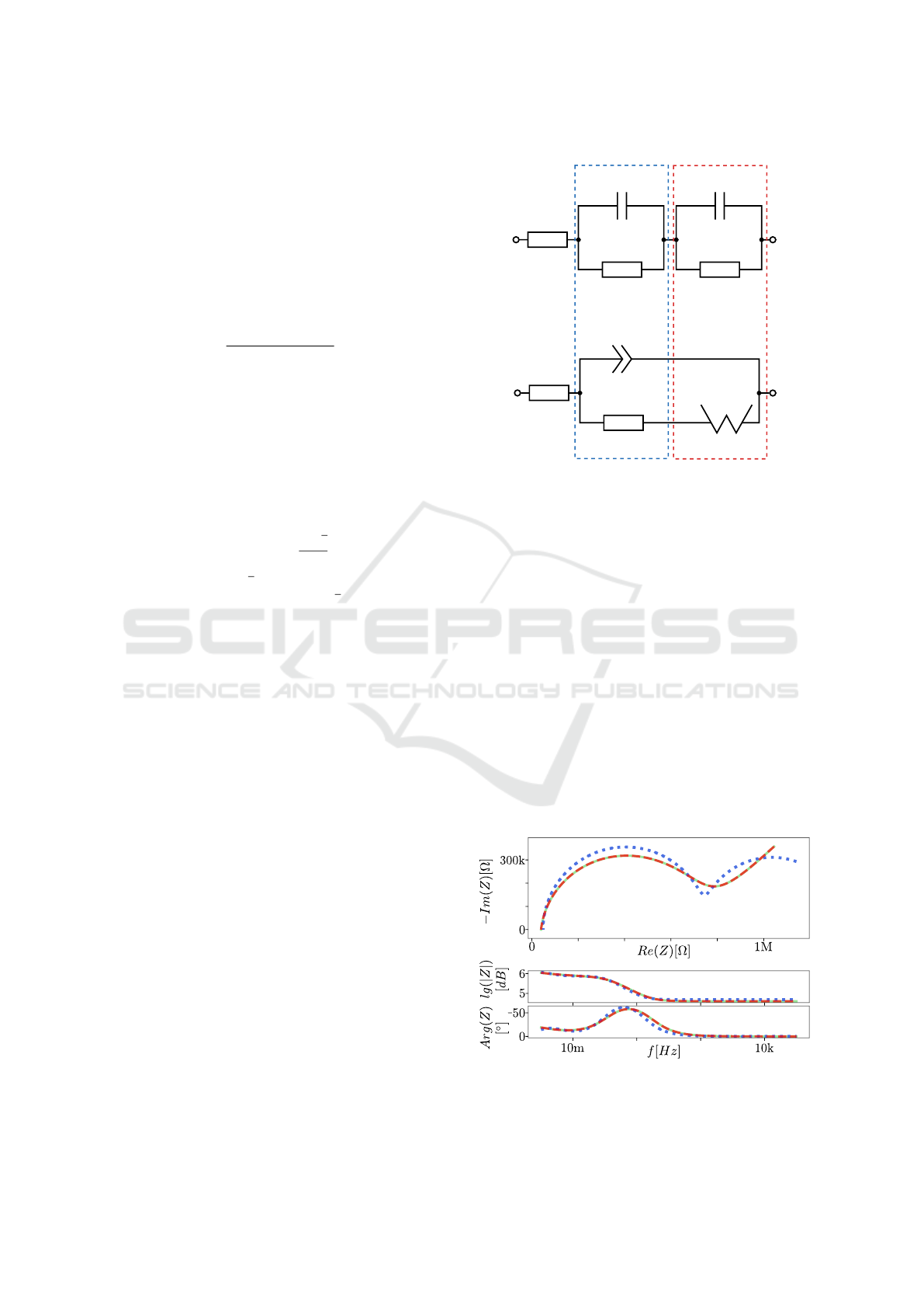
In general, the approach of the pre-fit is to perform
a CNLS with a circuit that contains a series connec-
tion of two RC elements (R
m
, C
m
for m = 1,2) and a
series resistor R
0
(see Figure 2). The result of the pre-
fit is then used as the start value for the actual CNLS
with the Randles circuit. Therefore, the components
from the pre-fit have to be assigned to the components
from the Randles circuit and can then be used as start
values for the CNLS. For this purpose, the time con-
stants of the determined RC elements are calculated
according to τ
m
= R
m
C
m
and sorted by size in ascend-
ing order.
R
s
R
ct
Z
w
CPE
R
0
R
1
C
1
R
2
C
2
m=1 m=2
Figure 2: Equivalent circuit diagram of the pre-fit approach
(top) with the corresponding assignment of the component
values to the parts of the Randles circuit (bottom). The as-
signment is done by means of the time constant τ
m
.
Using the τ
m
sorted by size, the elements of the
pre-fit can be assigned to the components of the Ran-
dles circuit. It is now exploited that τ for diffusion is
much larger than that of a charge exchange. First, R
s
is given by the series resistance R
0
. The remaining
components of the Randles circuit are then assigned
an ordinal number m. CPE and R
ct
form m = 1 and Z
w
is assigned m = 2. This ordinal number corresponds
to the time constants of the pre-fit, sorted by size.
Thus, the smaller time constant from the pre-fit
is assigned to the CPE and its capacitor value C
1
is
used as start value for Q (See Equation 1). Because
the exponent of the CPE cannot be assigned, it is al-
ways set to n = 0.75. The component R
ct
receives the
resistance value R
1
from the same RC element. The
Figure 3: Exemplary illustration of a simulated spectrum
(green) with the result of the pre-fit (blue) and the corre-
sponding result of the CNLS (red) in the Nyquist and Bode
plot.
Elliptical Fitting as an Alternative Approach to Complex Nonlinear Least Squares Regression for Modeling Electrochemical Impedance
Spectroscopy
45
second RC element and Z
w
are handled in the same
way.
In the investigations of this work, a normal CNLS
is performed first, whose start values are the loga-
rithmic means of the defined ranges. If this does
not lead to a satisfying result, the same is done with
a former pre-fitting, which is exemplarily shown in
Figure 3.
2.3 Elliptical Fitting
In case only the parameter R
ct
is of interest for sen-
sor analysis, a geometric approach based on ellipti-
cal fitting was developed. Here it is taken into ac-
count that the influence of the Warburg impedance
is only effective at comparably low frequencies. In
higher frequency ranges, the equivalent circuit results
in the parallel circuit R
ct
||CPE shifted by the series
resistor R
s
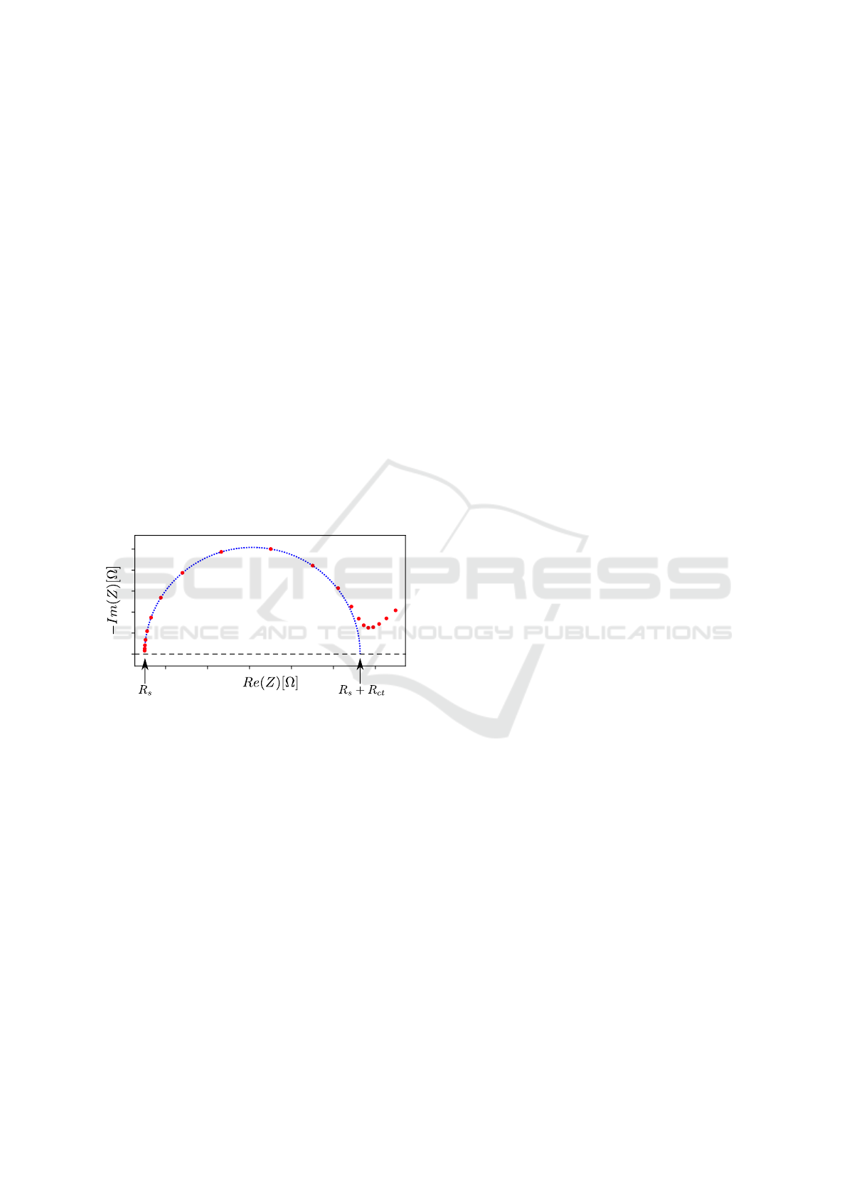
. Since this parallel circuit leads to a semi-
circle or a depressed semi-circle (Orazem and Tribol-
let, 2008) (Shoar Abouzari et al., 2009) with charac-
teristic points in the Nyquist plot (see Figure 4), an
elliptical fitting can be used to extract the value of R
ct
.
0
Figure 4: Exemplary Nyquist plot of a simulated data set
from a Randles circuit (red) with a fitted semicircle (blue).
The left zero crossing of the semicircle represents the R
s
,
the remaining zero crossing describes R
s
+ R
ct
.
In order to suppress the influence of the War-
burg impedance at lower measuring frequencies and
thus not to distort the fitting of the ellipse, a pre-
selection of measuring points is made. Only measur-
ing points on the semicircle at the Nyquist plot should
be used. The turning point between semicircle and
Warburg impedance is used as the cut-off point. To
find this point a 5th degree polynomial is fitted to the
impedance values of the Nyquist plot. This polyno-
mial degree has proven to be a good value to avoid
overfitting, but still to reproduce the curve as accu-
rately as possible. Starting from the polynomial, the
first and second derivatives are formed. The inflection
point now results from the zero point of the second
derivative, as far as the first derivative is positive. All
points to the left of this point are used for the ellipse
fit.
When a cone is cut on a plane that does not contain
the apex or is perpendicular to the axis of rotation, an
ellipse is obtained. A circle is only a special case of
an ellipse with half axes of equal size. For this reason
the basis for the fit is the general cone equation
F(~a,~x) = ax
2
+ bxy + cy
2
+ dx + ey + f = 0. (12)
Hereby, ~a =
a b c d e f
T
and
~x =
x
2
xy y
2
x y 1
T
(Fitzgibbon et al.,
1999). The algebraic distance F(a,x) is the dis-
tance of a point (x,y) from the intersection edge
F(a, x) = 0. Using the method of least squares this
distance shall be minimized for given data points. To
avoid trivial solutions like ~a = 0 additional conditions
have to be set to the solution. A simple approach
is the consideration as an eigenvalue problem. For
this a quadratic condition matrix C is set up. The
eigenvalue problem thus results in
D
T
Da = λCa (13)
with the design matrix D =
x
1
x
2
c... x
n
T
(Bookstein, 1979). C has the condition that the vec-
tor ~a must describe an ellipse. Fitzgibbon et al. de-
scibed that this can be achieved with a negative dis-
criminant b
2
−4ac (Fitzgibbon et al., 1999). This is
generally difficult to solve, but this application leaves
the freedom to scale the parameters arbitrarily. Thus
the equality constraint 4ac −b
2
= 1 is obtained. In
matrix notation the constraint can be written as
~a
T
C~a = 1 (14)
where
C =
0 0 2 0 0 0
0 −1 0 0 0 0
2 0 0 0 0 0
0 0 0 0 0 0
0 0 0 0 0 0
0 0 0 0 0 0
. (15)
The minimization problem can then be solved by cal-
culating the eigenvectors of the Equation 13. If now a
pair of eigenvalue and eigenvector (λ
i
,~u
i
) solves the
equation system, so does also (λ
i
,µ~u
i
) with each value
of µ. With the condition from Equation 14 we can
now find a value for µ thus resulting in
µ
2
i
~u
T
i
C~u
i
= 1. (16)
Accordingly, it applies that
BIOSIGNALS 2021 - 14th International Conference on Bio-inspired Systems and Signal Processing
46
µ
i
=
s
1
~u
T
i
C~u
i
. (17)
The parameters for an ellipse, which solves the opti-
mization problem, now result from
ˆa
i
= µ
i
~u
i
. (18)
3 RESULTS
Both approaches, the CNLS and the elliptical fitting
were applied to the simulated spectra. An exemplary
data set is shown in Figure 5.
Figure 5: Example of simulated data points of a Ran-
dles circuit with superimposed noise (blue; R
s
= 1.72 ·
10
4
, R
ct
= 2.10 ·10
6
, Q
w
= 2.83 ·10
−7
, Q = 3.13 ·10
−10
,
n = 0.88), the appropriate result of the model fitting (black;
−0.05% error of the R
ct
calculation) and of the elliptical
fitting (red, 0.26% error of the R
ct
calculation).
The calculated value of the parameter R
ct
were ex-
tracted and compared to the original value of the sim-
ulation. They were used to calculate the mean rela-
tive error E
R
and the coefficient of determination R
2
.
The simulated spectra, which could not be fit by one
of the presented approaches, were discarded for fur-
ther investigation. The raw and noisy data were con-
sidered separately. To compare the performance of
both approaches, the required calculation times were
measured for each fitting procedure. All methods are
implemented in the Python programming language.
The simulations were performed on a 1.90 GHz Intel
®
Core™ i7-8650U Prozessor with 16 GB of RAM.
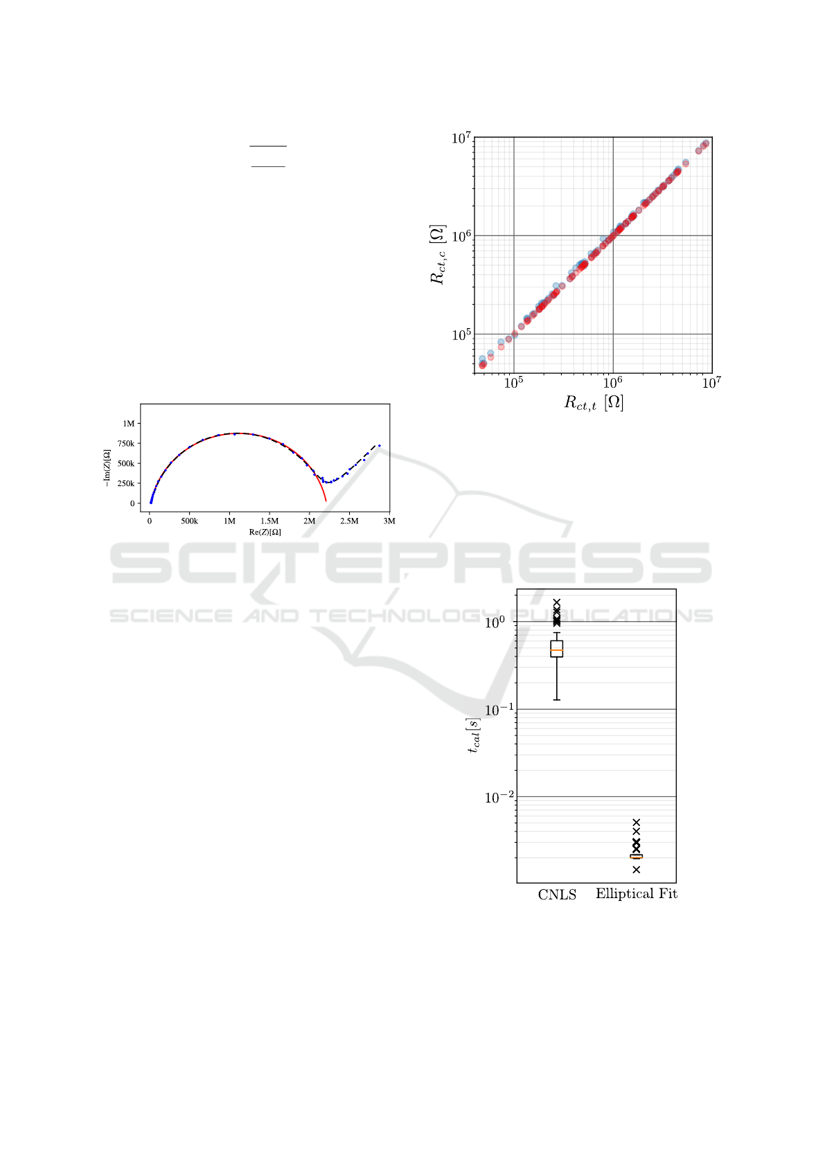
The achieved results for both methods are shown
in Table 2. The relative Error E
R
represents the differ-
ence between the calculated value R
ct,c
and the true
value R
ct,t
, referred to R
ct,t
. The linear relationship
R
ct,c
= mR
ct,t
+b with its coefficient of determination
R
2
were calculated and is exemplary shown in
Figure 6 for the noisy spectra. Table 2 also shows the
number of discarded spectra N
d
which could not be
fitted with the presented approaches.
Figure 6: Linear relationship between the calculated values
R
ct,c
of the CNLS (red) or the elliptical fitting (blue) and the
true value R
ct,t
.
The calculation time for each approach was mea-
sured, whereby all steps depending on the method
(e.g. preselection of measuring points, normalization,
fitting) were included. The distribution of the calcu-
lation times is shown as boxplot for the raw spectra in
Figure 7.
Figure 7: Distribution of the calculation time for CNLS and
the elliptical fitting. 100 raw spectra without noise were
used.
Elliptical Fitting as an Alternative Approach to Complex Nonlinear Least Squares Regression for Modeling Electrochemical Impedance
Spectroscopy
47

Table 2: Results of the simulation of the CNLS and the elliptical fiting EF. Raw signals (CNLS
r
,EF
r
) and noisy signals
(CNLS
n
,EF
n
) were observed. The parameters mean relative error E
R
, slope m, intercept b, coefficient of determination R
2
,
number of discarded spectra N
d
, median calculation time t
cal
were determined.
E
R
[%] m b[Ω] R
2
N
d
t
cal
[s]
CNLS
r
1.5 ·10
−6
±1.5 ·10
−5
1.00000 1.2 ·10
−3
1.00000 1 4.6 ·10
−1
EF
r
−2.7±4.2 1.01027 5.6 ·10
3
0.99957 2 2.0 ·10
−3
CNLS
n
2.4 ·10
−2
±4.6 ·10
−1
0.99934 5.3 ·10
2
0.99997 0 4.5 ·10
−1
EF
n
−2.7±4.3 1.00965 5.6 ·10
3
0.99950 2 2.0 ·10
−3
4 DISCUSSION AND OUTLOOK
By using the CNLS, low error in the calculation of R
ct
is achieved and also the linear relationship to the real
value is better compared to the elliptical fitting at least
for non-noisy spectra. However, this difference in
performance is smaller when considering noisy spec-
tra. This observation leads to the assumption that for
very noisy signals the difference between the two ap-
proaches could become even smaller. However, this
has to be investigated and evaluated in the following
work, preferably by using real measured spectra from
FET-based biosensors. Besides the consideration of
different noise overlays, the analysis of artifact influ-
ences would also be relevant.
The results of the time measurements show that
the elliptical fitting is more resource efficient than
CNLS. However, these results have to be interpreted
in the context of the normalization that has been car-
ried out for the CNLS. In this process, all components
of the equivalent circuit diagram are replaced by a
factor a and an exponent b (see Equation 9), which
in turn makes the regression more time-consuming.
Nevertheless, the elliptical fitting might be more suit-
able to be implemented on low-power embedded sys-
tems. In this respect, further concepts have to be de-
veloped how this approach can be efficiently imple-
mented on an embedded system. Thus an investiga-
tion of the power consumption would be applicable
as well.
Although the elliptical fitting requires less com-
putational time than the CNLS, it is also able to fit
the majority of the spectra within the data set consid-
ered in this work, which in turn stands for a high ro-
bustness of the algorithm. However, the CNLS with
the pre-fit algorithm achieves even better results but
with a greater computational effort. It should be em-
phasized that the pre-fit was mainly responsible for
achieving these good values, since without the pre-
fit the CNLS would have had to reject 33 spectra
(without noise) or respective 31 spectra (with noise).
It is also striking that the superimposed noise has a
positive effect on the modeling ability of the CNLS,
although a strong vulnerability to noise has already
been described in the literature (Kauffman, 2009).
The results also confirm that start values of the com-
ponents are decisive for the error obtained with CNLS
and demonstrate the effectiveness of the pre-fit algo-
rithm. However, the disadvantage of a high depen-
dency on the start values applies less strongly to the
elliptical fitting. Nevertheless, further optimizations
of the elliptical fitting should be implemented, allow-
ing to reliably fit more spectra. This can be achieved
by intercepting cases where the Warburg impedance
already dominates at the imaginary maximum of the
semicircle, causing the pre-selection of measurement
points to be erroneous.
For a real application scenario, the presented ap-
proaches should be adapted in order to optimize their
performance. For example, due to smaller min-max
limits of the individual parameters, particular expo-
nents can be fixed so that the regression is less com-
putationally demanding. However, the presented ap-
proaches allow the modelling of a wide range of pa-
rameter combinations without the need to specify ap-
proximate initial values or narrower limits for extreme
values. They thus represent generic modelling tech-
niques.
In cases where C
dl
can be applied instead of CPE,
the semicircle of the Randles circuit is not depressed.
For this purpose, further research is needed to deter-
mine the accuracy and computational effort that can
be achieved by a circular fitting.
5 SUMMARY
With an average error of −2.7%, the elliptical
fitting cannot achieve the accuracy of the CNLS
(2.4 ·10
−2
%) for the determination of R
ct
, at least
when using ideal spectra. Thereby it could be shown
that pre-fit is a suitable method to reduce the depen-
dence of CNLS on the start value. Preliminary data
indicate that the results of elliptical fitting are less de-
pendent on noise than CNLS, but in any case, the lat-
BIOSIGNALS 2021 - 14th International Conference on Bio-inspired Systems and Signal Processing
48

ter has lower errors and a lower number of rejected
spectra for the data used in this work. However, this
behavior needs further investigation. The measure-
ments of the computation time showed that the el-
liptical fitting needs only about
1
/225 of the compu-
tational effort compared to the CNLS. This leads to
the assumption that this approach might be suitable
for implementations on embedded systems. For this
purpose the accuracy of the elliptical fitting has to be
estimated depending on the application, the measure-
ment and/or the sensor.
ACKNOWLEDGEMENTS
This research was funded by EU H2020 research and
innovation program entitled KardiaTool with grant
N
o
768686.
REFERENCES
Barsoukov, E. and Macdonald, J. R. (2005). Impedance
Spectroscopy: Theory, Experiment, and Applications.
Barsukov, Y. and Macdonald, J. R. (2012). Electrochemi-
cal Impedance Spectroscopy, pages 1–17. American
Cancer Society.
Bertsekas, D. P. (1999). Nonlinear programming, Second
Edition.
Bookstein, F. L. (1979). Fitting conic sections to scattered
data. Computer Graphics and Image Processing.
Chowdhury, A. D., Ganganboina, A. B., Park, E. Y., and
an Doong, R. (2018). Impedimetric biosensor for de-
tection of cancer cells employing carbohydrate target-
ing ability of Concanavalin A. Biosensors and Bio-
electronics.
Cimafonte, M., Fulgione, A., Gaglione, R., Papaianni, M.,
Capparelli, R., Arciello, A., Censi, S. B., Borriello,
G., Velotta, R., and Ventura, B. D. (2020). Screen
printed based impedimetric immunosensor for rapid
detection of Escherichia coli in drinking water. Sen-
sors (Switzerland).
Dang, W., Manjakkal, L., Navaraj, W. T., Lorenzelli, L.,
Vinciguerra, V., and Dahiya, R. (2018). Stretchable
wireless system for sweat pH monitoring. Biosensors
and Bioelectronics.
Fitzgibbon, A., Pilu, M., and Fisher, R. B. (1999). Direct
least square fitting of ellipses. IEEE Transactions on
Pattern Analysis and Machine Intelligence.
Halima, H. B., Zine, N., Gallardo-Gonzalez, J., Aissari,
A. E., Sigaud, M., Alcacer, A., Bausells, J., and Er-
rachid, A. (2019). A Novel Cortisol Biosensor Based
on the Capacitive Structure of Hafnium Oxide: Appli-
cation for Heart Failure Monitoring. In 20th Interna-
tional Conference on Solid-State Sensors, Actuators
and Microsystems and Eurosensors.
Kauffman, G. B. (2009). Electrochemical Impedance Spec-
troscopy. By Mark E. Orazem and Bernard Tribollet.
Angewandte Chemie International Edition.
Kharitonov, A. B., Wasserman, J., Katz, E., and Willner,
I. (2001). The use of impedance spectroscopy for
the characterization of protein-modified ISFET de-
vices: Application of the method for the analysis of
biorecognition processes. Journal of Physical Chem-
istry B.
Leva-Bueno, J., Peyman, S. A., and Millner, P. A. (2020). A
review on impedimetric immunosensors for pathogen
and biomarker detection. Medical Microbiology and
Immunology.
Macdonald, D. D. (1990). Some advantages and pitfalls of
electrochemical impedance spectroscopy. Corrosion.
Orazem, M. E. and Tribollet, B. (2008). Electrochemical
Impedance Spectroscopy. Wiley.
Papageorgiou, M., Leibold, M., Buss, M., Papageorgiou,
M., Leibold, M., and Buss, M. (2015). Methode der
kleinsten Quadrate. In Optimierung.
Pejcic, B. and De Marco, R. (2006). Impedance spec-
troscopy: Over 35 years of electrochemical sensor op-
timization. Electrochimica Acta.
Prodromidis, M. I. (2010). Impedimetric immunosensors-A
review. Electrochimica Acta.
Randviir, E. P. and Banks, C. E. (2013). Electrochemi-
cal impedance spectroscopy: An overview of bioan-
alytical applications. Analytical Methods, 5(5):1098–
1115.
Rushworth, J. V., Ahmed, A., Griffiths, H. H., Pollock,
N. M., Hooper, N. M., and Millner, P. A. (2014).
A label-free electrical impedimetric biosensor for
the specific detection of Alzheimer’s amyloid-beta
oligomers. Biosensors and Bioelectronics.
Sgobbi, L. F., Razzino, C. A., and Machado, S. A. (2016).
A disposable electrochemical sensor for simultaneous
detection of sulfamethoxazole and trimethoprim an-
tibiotics in urine based on multiwalled nanotubes dec-
orated with Prussian blue nanocubes modified screen-
printed electrode. Electrochimica Acta.
Shoar Abouzari, M. R., Berkemeier, F., Schmitz, G., and
Wilmer, D. (2009). On the physical interpretation of
constant phase elements. Solid State Ionics, 180(14-
16):922–927.
Sun, A., Venkatesh, A. G., and Hall, D. A. (2016). A Multi-
Technique Reconfigurable Electrochemical Biosen-
sor: Enabling Personal Health Monitoring in Mobile
Devices. IEEE Transactions on Biomedical Circuits
and Systems.
Willa, C., Schmid, A., Briand, D., Yuan, J., and Koziej,
D. (2017). Lightweight, Room-Temperature CO2 Gas
Sensor Based on Rare-Earth Metal-Free Composites
- An Impedance Study. ACS Applied Materials and
Interfaces.
Yuan, X.-Z., Song, C., Wang, H., and Zhang, J. (2010).
Electrochemical Impedance Spectroscopy in PEM
Fuel Cells. Springer, London.
Elliptical Fitting as an Alternative Approach to Complex Nonlinear Least Squares Regression for Modeling Electrochemical Impedance
Spectroscopy
49
