Generating Reactive Robots’ Behaviors using Genetic Algorithms

Jesus Savage

, Stalin Mu

noz

, Luis Contreras

, Mauricio Matamoros

, Marco Negrete

Carlos Rivera

, Gerald Steinbabuer

, Oscar Fuentes

and Hiroyuki Okada

Bio-Robotics Laboratory, School of Engineering, National Autonomous University of Mexico (UNAM), Mexico

Graz University of Technology, Austria

Advance Intelligence and Robotics Research Center, Tamagawa University, Japan

Keywords:

Evolutionary Algorithms, Robot Behaviors, Finite State Machines, Hidden Markov Models.

Abstract:

In this paper, we analize and benchmark three genetically-evolved reactive obstacle-avoidance behaviors for

mobile robots. We buit these behaviors with an optimization process using genetic algorithms to ﬁnd the one

allowing a mobile robot to best reactively avoid obstacles while moving towards its destination. We compare

three approaches, the ﬁrst one is a standard method based on potential ﬁelds, the second one uses on ﬁnite

state machines (FSM), and the last one relies on HMM-based probabilistic ﬁnite state machines (PFSM). We

trained the behaviors in simulated environments to obtain the optimizated behaviors and compared them to

show that the evolved FSM approach outperforms the other two techniques.

1 INTRODUCTION

In the many years of research on robot navigation sev-

eral algorithms for robot exploration in unknown en-

vironments have been proposed, many of them based

on Finite State Machines (FSM) (Fraundorfer and

Scaramuzza, 2012). In these algorithms, a robot with

negligible errors in both, the sensor readings and its

motion, under the same initial conditions, should be-

have always in the same way due to the deterministic

nature of its control algorithm.

While this behavior ﬁts most applications, the ex-

ploration of new environments makes desirable for

the robot to behave differently every time under simi-

lar conditions (for example, to construct a complete

map of a scene by aggregating unexplored areas).

Therefore a probabilistic ﬁnite state machine is used.

Consequently, we built these state machines using a

modiﬁed version of Hidden Markov Models (HMM)

and we proposed an optimization process to ﬁnd the

best HMM model using Genetic Algorithms (GA).

The paper is organized as follows: in Section 2

we present the related work in this area. Section 3

presents the standard robot behavior of potential ﬁelds

to be compared with the behaviors proposed in this

paper. Meanwhile, in Section 4 we detail how to cre-

ate navigation behaviors using FSM. Then, in Sec-

tion 5 we present the Probabilistic Finite State Ma-

chines (PFSM) using HMM. Further, in Section 6 we

explain how we got the ﬁttest behaviors for the po-

tential ﬁelds approach, the FSM and the PFSM using

Genetic Algorithms. Finally, in Section 7 we detail

the experiments and results, and close in Section 8

with the conclusions of this work.

2 RELATED WORK

Brooks proposed a new robotics paradigm to con-

trol robots in which their behaviors are built using

Augmented Finite State Machines (AFSM) (Brooks,

1986). To Brooks, by connecting together the AFSM,

each one containing a behavior, emergent intelligence

can be achieved by a robot.

Simulated emergent patterns from a collection of

artiﬁcial agents refers back to Barricelli (1954). In

this work, as refereed by Fogel (2006), Barricelli sim-

ulates an early version of cellular automaton in which

numbers, that live in one and two dimensional worlds,

interact following simple rules. His computer simula-

tions showed that such simple rules are sufﬁcient to

give rise to regular patterns which he called “organ-

isms”.

Meanwhile, starting in 1962, Lawrence J. Fogel

and colleagues successfully applied artiﬁcial evolu-

tion algorithms to the problem of ﬁnding predictions

in sequences of symbols in ﬁnite alphabets (Fogel,

698

Savage, J., Muñoz, S., Contreras, L., Matamoros, M., Negrete, M., Rivera, C., Steinbabuer, G., Fuentes, O. and Okada, H.

Generating Reactive Robots’ Behaviors using Genetic Algorithms.

DOI: 10.5220/0010229306980707

In Proceedings of the 13th International Conference on Agents and Artiﬁcial Intelligence (ICAART 2021) - Volume 2, pages 698-707

ISBN: 978-989-758-484-8

 2021 by SCITEPRESS – Science and Technology Publications, Lda. All r ights reserved

2006). In their work, they used ﬁnite state machines

to represent the behavior of the agent (Fogel, 2006).

This early evolutionary algorithm uses a population

of states machines and exploits several kinds of mu-

tations to generate the offspring. The task to solve

was to predict whether the next number in a sequence

will be a prime number or not. The algorithm quickly

learned to discriminate even numbers and numbers di-

visible by three as non-prime and achieved a 78% of

prediction accuracy.

In (Negrete et al., 2018), from a red, green, blue

and distance (RGBD) sensor, as the Kinect, a differ-

ent map representation is used where the free space is

divided into regions using vector quantization where

each centroid represents a node in a topological map

useful for robot navigation, where quantization has

been proven to be the state-of-the-art for scaling the

search space (Guo et al., 2020). A probabilistic map

representation has been proposed in (Savage et al.,

2018) where we represent the current pose with a Hid-

den Markov Model and determine the next navigation

node by incorporating new laser readings and the all

trajectory information into the model; therefore, al-

though reactive, this approach produces smooth tra-

jectories. Probabilistic representation given by a Hid-

den Markov Model from a number of sensor read-

ings and robot displacements have been proven use-

ful for robot localization and navigation (Shahriar and

Zelinsky, 1999), (Shahriar and Zelinsky, 2014), and

(Mohanan and Salgaonkar, 2020). Furthermore, path

planning in mobile robots is a very well known prob-

lem and Genetic Algorihms have been widely applied

to solve this problem (Yakoubi and Laskri, 2016) and

(Yakoubi and Laskri, 2018).

3 ROBOT BEHAVIORS USING

POTENTIAL FIELDS

In this type of behavior, the robot is modeled as a

particle that is under the inﬂuence of two potential

ﬁelds, one attracts it towards the destination, while an-

other takes him away from obstacles (Latombe et al.,

1991). Obstacles exert repulsive forces, while the

goal destination generates and attraction force. The

robot moves through a potential ﬁeld on the steepest

slope until it brings it to the destination.

The robot position in the environment is

= [x

], and the potential ﬁeld exerted on the

robot at that point is:

U(q) = U

atr

(q) +U

rep

(q)

the gradient of the potential ﬁeld:

F(q) = ∇U(q) =



∂U

∂x

i +

∂U

∂y



using the “steepest descent” technique the next posi-

tion of the robot is given by:

= q

n−1

− δ



n−1



where δ

are constants that determine the size of the

robot advance, sometimes it remains ﬁxed.



n−1



is a unit force vector in the direction of

the gradient:

f (q

n−1

) =

F(q

n−1

)



F(q

n−1

)



The robot moves following the steepest slope of the

potential ﬁeld, given by the forces of attraction and

repulsion:

F(q

n−1

) =F

atr

n−1

) + F

rep

n−1

)

n−1

− δ



n−1



3.1 Attraction Field

The destination that the robot needs to reach is:

dest

= (x

dest

)

We deﬁne the attractive ﬁeld of parabolic type as:

atr

(q) =

|q − q

dest

where ε

it is a constant that modulates the ﬁeld and

is found empirically. The attractive force in q is:

∇U

atr

(q) = ε

[q − q

dest

] = F

atr

(q)

3.2 Repulsive Fields

We deﬁne the repulsive ﬁeld as:

rep

(q) =



|q − q

obs

−



where q

obs

= (x

obs

) is the obstacle centroid

position. This repulsion ﬁeld applies when

|q − q

obs

| ≤ d

. Otherwise, it is considered that the

obstacle does not generate any repulsive force be-

cause it is too far away. Where η is a constant that

modulates the ﬁeld and is found empirically. Then

the potential ﬁeld is:

Generating Reactive Robots’ Behaviors using Genetic Algorithms

699

∇U

rep

(q) = −η



q − q

obs

−



q − q

obs

q − q

obs

= F

rep

(q)

The repulsion force generated by the obstacle k

rep

(q) = 0 if



q − q

obs



> d

the total force exerted on the robot in the position q

is:

F(q) = F

atr

(q) +

∑

k=1

rep

(q)

where N is the number of obstacles in the environment

where the robot navigates.

The new position of the robot is given by the fol-

lowing equation:

= q

n−1

− δ



n−1



For the potential ﬁeld approach it is necessary to ﬁnd

the constants that control this behavior, namely η,ε

and d

4 DETERMINISTIC FINITE

STATE MACHINES

In mobile robots, behaviors are often used for navi-

gation (Arkin, 1998). These methods can be imple-

mented using ﬁnite state machines FSM.

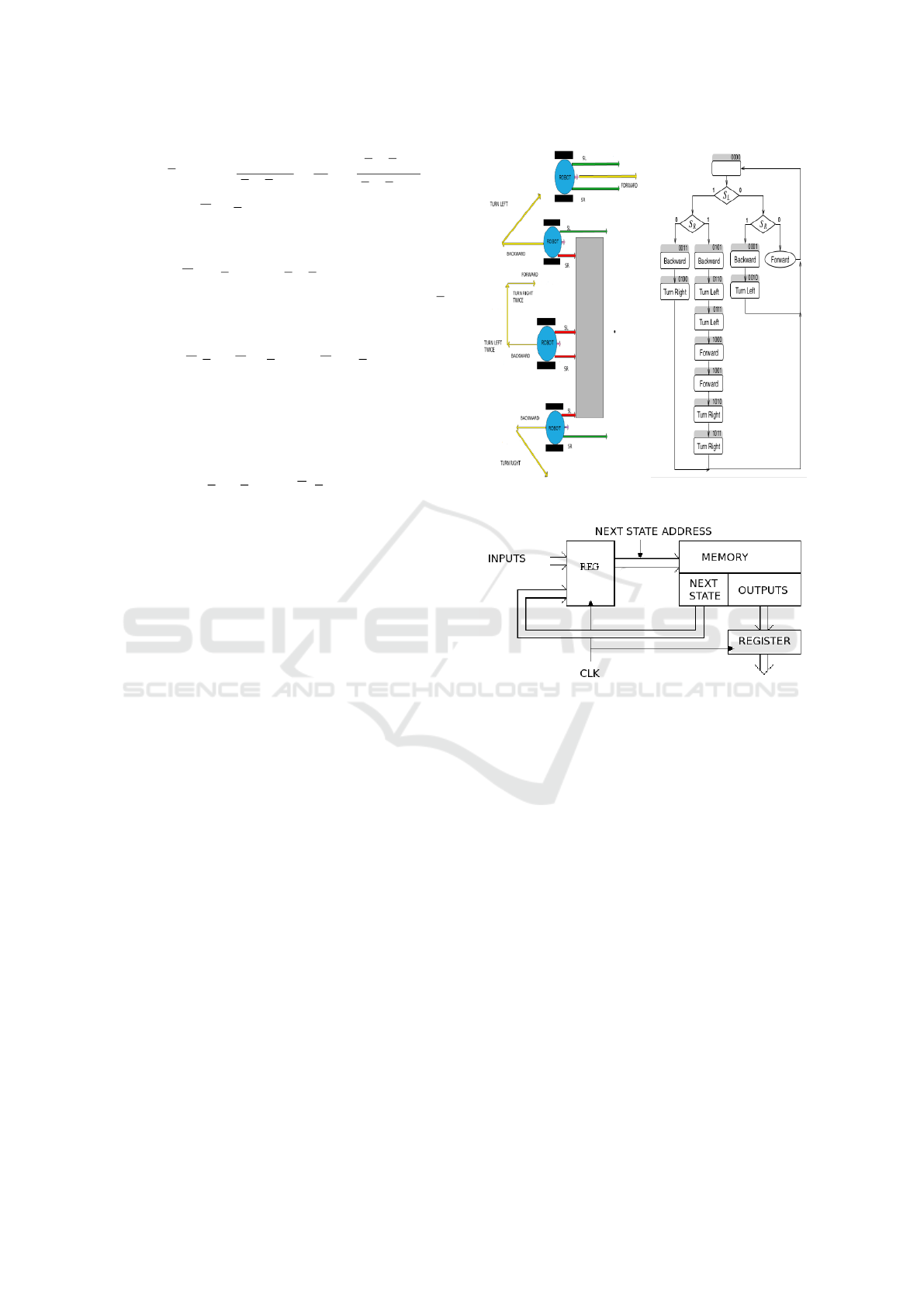
Figure 1 shows a simple behavior for a robot

whose goal is to avoid obstacles on its path. The robot

has two proximity sensors, one on its left (LS) and one

on its right side (RS), allowing it to detect obstacles.

The sensors are binary and return 1 when an obstacle

is detected within their range. The robot has two mo-

tors for propulsion in differential pair conﬁguration.

Figure 1 shows the algorithm state machine

(ASM) for the obstacle avoidance behavior shown in

the same ﬁgure.

There are many ways to physically implement the

obstacle avoidance behavior using of state machines.

One option is to use standard memories. Figure 2

shows an architecture of a state machine that uses a

memory. In it, the ASM is encoded in a look-up ta-

ble that contains the next state and the outputs of each

state. The inputs of the state machine, sensors, and

the next state are linked together to form the address

of the memory that contains the next state and outputs

for the present state.

This type of architecture can be implemented in a

FPGA for robots with small computational resources,

but also can be implemented using a look-up table in

Figure 1: Robot avoiding an obstacle.

Figure 2: Implementation of an State Machine Using Mem-

ories.

high level languages as C/C++, Python, etc. Using

this method, depending of the number of states N

each state is represented by N

= dlog

)e bits. The

number of memory locations used is 2

)

, where

is the number of inputs. Figure 1 shows the ASM

with 12 states and with two inputs.

Table 1 shows the coding of the actions the mobile

robot can perform:

Using this method, each state is represented by

= dlog

)e bits where N

is the number of states.

The number of memory locations used is 2

)

where N

is the number of inputs.

Table 1 below shows the coding of the actions the

mobile robot can perform:

The number of bits to encode the outputs is N

dlog

(Num.Actions)e Thus each memory location re-

quires N

+ N

bits to indicate the next state and the

robot’s actions. The obstacle avoidance algorithm

shown in Figure 1, requires four memory locations

to represent each state, to select the memory location

the 4 bits that represent the states and the 2 bits for the

ICAART 2021 - 13th International Conference on Agents and Artiﬁcial Intelligence

700

Table 1: Robot Action Coding.

Robot Action Binary Code

Stop 000

Forward 001

Backward 010

Turn Left (45

◦

) 011

Turn Right (−45

◦

) 100

Turn Left (45

◦

) and Forward 101

Turn Right (45

◦

) and Forward 110

Turn Right Twice (90

◦

) and For-

ward

111

inputs are concatenated to form the memory address,

then the total number of memory locations necessary

is 64, with a width of each location of 7 bits.

For the ASM shown in Figure 1, the state 0 has

one conditional output (Forward) shown inside the

oval. This output is generated when both inputs LS

and RS are zero. For any the other cases the robot

will Stop. The inputs LS and RS represent the digital

value from the sensors. Table 2 shows the encoding

of this state 0.

Table 2: AFSM MEMORY.

Pr. State S

Inputs Next State S

t+1

Outputs

A B C D LS RS ABCD b

0 0 0 0 0 0 0 0 0 0 0 0 1

0 0 0 0 0 1 0 0 0 1 0 0 0

0 0 0 0 1 0 0 0 1 1 0 0 0

0 0 0 0 1 1 0 1 0 1 0 0 0

As we can see in Table 2 changing one of the bits of

the memory will change the algorithm hance also the

robot’s behavior. For instance, in the third row of Ta-

ble 2, if two bits of the memory contents are randomly

changed as in Table 3, the state machine will jump to

est

instead of state est

given the same conditions,

generating therefore a Turn Right output instead of a

Stop one.

Thus, one of the goals is to ﬁnd the best conﬁgura-

tion of the memory content to get a robot’s behavior.

Table 3: Third raw State 0 AFSM MEMORY.

Pr. State S

Inputs Next State S

t+1

Outputs

A B C D LS RS ABCD b

0 0 0 0 1 0 1 0 1 1 1 0 0

Without or small errors in the sensing and in the

movements the robot, under the same conditions, that

is, with the same initial pose, x

,θ

and same des-

tination x

, the robot should behave always in the

same way, because the algorithm that control it it

is deterministic. While this type of behavior is de-

sired for some robotics applications, in others it would

be desired that the robot behaves in a different way

each time under similar conditions, thus a probabilis-

tic FSM is used. This kind of state machines are build

using HMM, as it is explained in the next section.

5 PROBABILISTIC FINITE STATE

MACHINES

The algorithm of a Probabilistic Finite State Ma-

chines (PFSM) depends on random variables (Vidal

and Thollard, 2005) and therefore it can be model us-

ing Hidden Markov Models (HMM). In this section,

we explain our approach to this problem, referred as

the Behavior HMM, and later it is explained how

we optimize this model through Genetic Algorithms

(GA).

5.1 Hidden Markov Models

A HMM is a doubly stochastic process, in which the

set of states S is hidden and the set of symbols O are

observable (Rabiner and Juang, 1986). The stochas-

tic process exhibits the Markov property, that is, the

probability of reaching a particular next-state depends

only on the current state and not in the whole history

of the process. States are not directly observable and

can only be inferred by their probabilistic emission of

observable symbols.

The observation symbols are V = (V

,...,V

And the probability of emitting symbol k being in

state i, b

(k) = p(O

= k|S

= i), where S

= i means

the Markov chain was in state i at time t, and O

= k

means the observed symbol at time t was k.

The transition probability deﬁnes the probability

of taking the transition from a particular state to an-

other state or itself. Where a

i j

is the probability of

taking a transition from state i to state j:

i j

= p(S

t+1

= j|S

= i).

Also included is the initial state distribution probabil-

ity:

= P[s

= S

], 1 <= i <= N

A standard Markov model is formed by a structure

called λ = (A,B,π), where A and B are two matrices

with components: A = (a

i j

), B = (b

) for all i, j and

k, with N states and L observation symbols; and π.

Generating Reactive Robots’ Behaviors using Genetic Algorithms

701

5.2 Discrete Hidden Markov Models for

Robots Behaviors

In this work, we propose a probabilistic representa-

tion of the algorithm’s FSM by a HMM, in this, the

states are part of a probabilistic state machine, that

have the similar characteristics as the states in the

deterministic ones, but taking into consideration the

stochastic behavior of the system. There is a direct

matching between the inputs of the FSM, becoming

observations in a HMM, and also for the transitions

from one state to another. The inputs in the determin-

istic FSM become the observation in the HMM. That

is, the observation symbols are formed by quantized

version of the input sensors as is explained in Sec-

tion 5.5.

The decision to change to another state depends on

the present state S

, the observed symbol O

at time t

and the λ model of the HMM.

Given a HHM model λ = (A, B, π) with N states

and L observation symbols, and with the system been

in states {S

...S

t−2

t−1

}, past observation sequence

{O = O

,...,O

t−1

} and a new observation O

, to

ﬁnd which will be the next state s

at time t, it is nec-

essary to calculate the maximum transition probabil-

ity of going from any state i to j:

( j) = max

1<i<N

P[S

...S

t−1

= i, O

,...,O

|λ] (1)

where

1 < j < N

that is, δ

( j) keeps the highest probability of reaching

state j, and this calculation is done with all states 1 <

i < N. This is similar to the calculations used by the

Viterbi algorithm (Viterbi, 1967; Rabiner and Juang,

1986) to ﬁnd the best sequence of states that reaches

a particular state, the difference with our approach is

that we want to predict which is the most probable

next state. Then the most probable next one is:

= j = arg max

1<i<N

[δ

(i)]

This equation can be calculated recursively, with the

following procedure:

Initialization:

(i) = π

), 1 < i < N, (2)

= j = arg max

1<i<N

[δ

(i)] (3)

Recursion:

( j) = max

1<i<N

[δ

t−1

(i)a

i j

), 1 < j < N (4)

= j = arg max

1<i<N

[δ

(i)] (5)

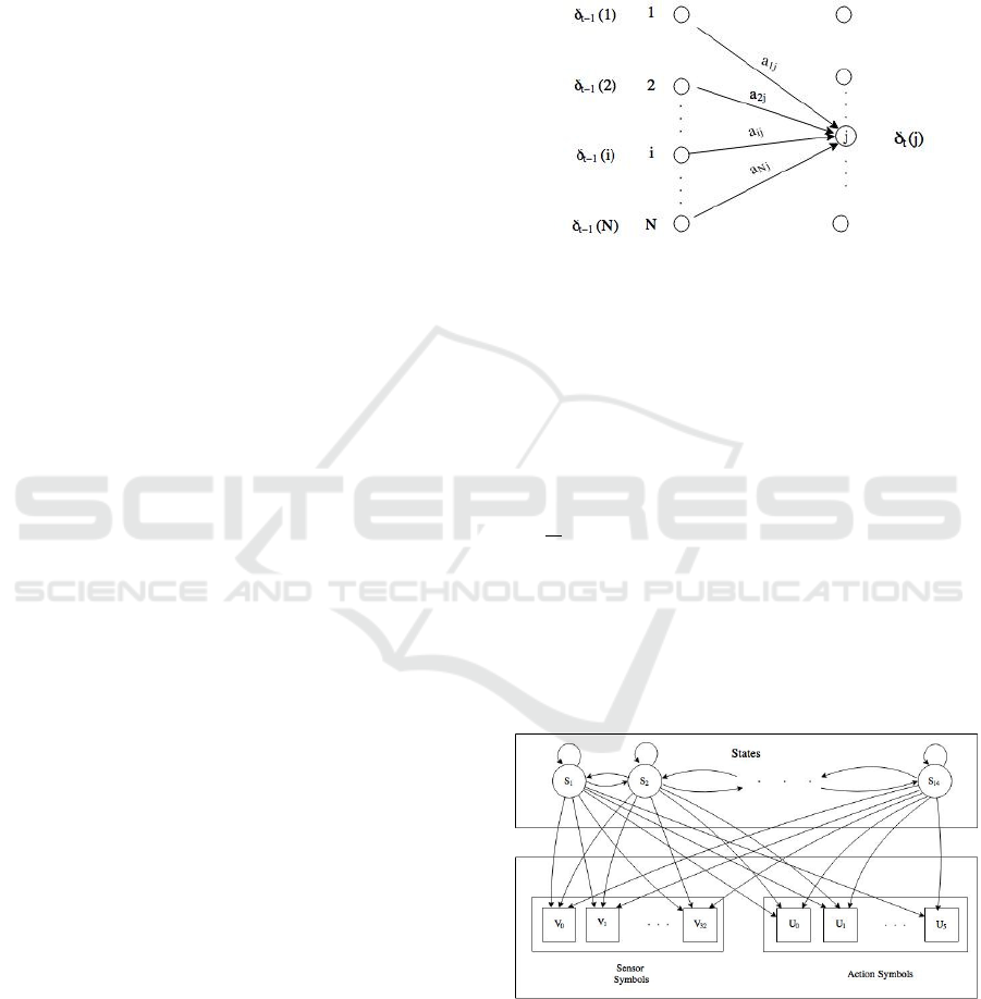
Figure 3 shows each state having a δ

t−1

at time t − 1

and at time t, for each state j, δ

( j) needs to be calcu-

lated again, by taking into consideration the transition

probabilities a

i j

and the symbols probabilities b

Figure 3: Best next state j given by δ

( j).

Thus, matrix B needs to be created taking into con-

sideration equation Equation (4).

5.3 Action Symbols

In our approach, we incorporate the outputs of the

FSM as action symbols attached to the states of the

HMM. The action symbols are:

U = { Stop, Forward, Backward, Turn Left (45

◦

Turn Right (−45

◦

), Turn Left and Forward, Turn

Right and Forward, Turn Right twice (−90

◦

) and For-

ward} = {U

Figure 4 shows the structure of the HMM taking into

consideration the sensor symbols (FSM inputs) and

the action symbols (FSM outputs).

Figure 4: Extended version of an HMM, the sensor inputs

and the robot’s actions are incorporated in the HMM.

Thus, we needed to incorporate matrix C, into the

robot’s behavior model HMM λ = (A,B,C,π), that

contains the probability of generate an action AC

given that we are on state S

= j and with observa-

tion O

= Vi:

ICAART 2021 - 13th International Conference on Agents and Artiﬁcial Intelligence

702

Let C = c

l,k

such as l = concat ( j,i) where concat

is a bit concatenation operation, j is the index of the

state S

and i is the index of observation O

l,k

= p(U

= k|S

= j,O

= i).

To form the C matrix’s rows indices is a concatenation

of the state’s index j together with the observation in-

dex i.

We call this new type HMM model λ = (A,B,C,π)

an extended HMM (EHMM).

5.4 Execution of the Behavior HMM

To start the execution of the probabilistic state ma-

chine, given the robot’s behavior model EHMM, λ =

(A,B,C,π), ﬁrst the robot needs to make an observa-

tion at time t = 1, O

, and then to calculate the fol-

lowing equations to ﬁnd the ﬁrst state:

(i) = π

), 1 < i < N, (6)

= j = arg max

1<i<N

[δ

(i)] (7)

Once the ﬁrst state is calculated then the output ac-

tion needs to be found, due to the stochastic nature of

the probabilistic state machine, the output is not just

generated using the action symbol with the highest

probability in that state, but by generating a random

number and comparing in which region it is of all pos-

sible outputs in a particular case. In our approach, the

row of matrix C to be used in the calculation of the

probabilities of the output is by a concatenation of the

state’s index j together with the observation index i.

With this row, a range of the outputs symbol proba-

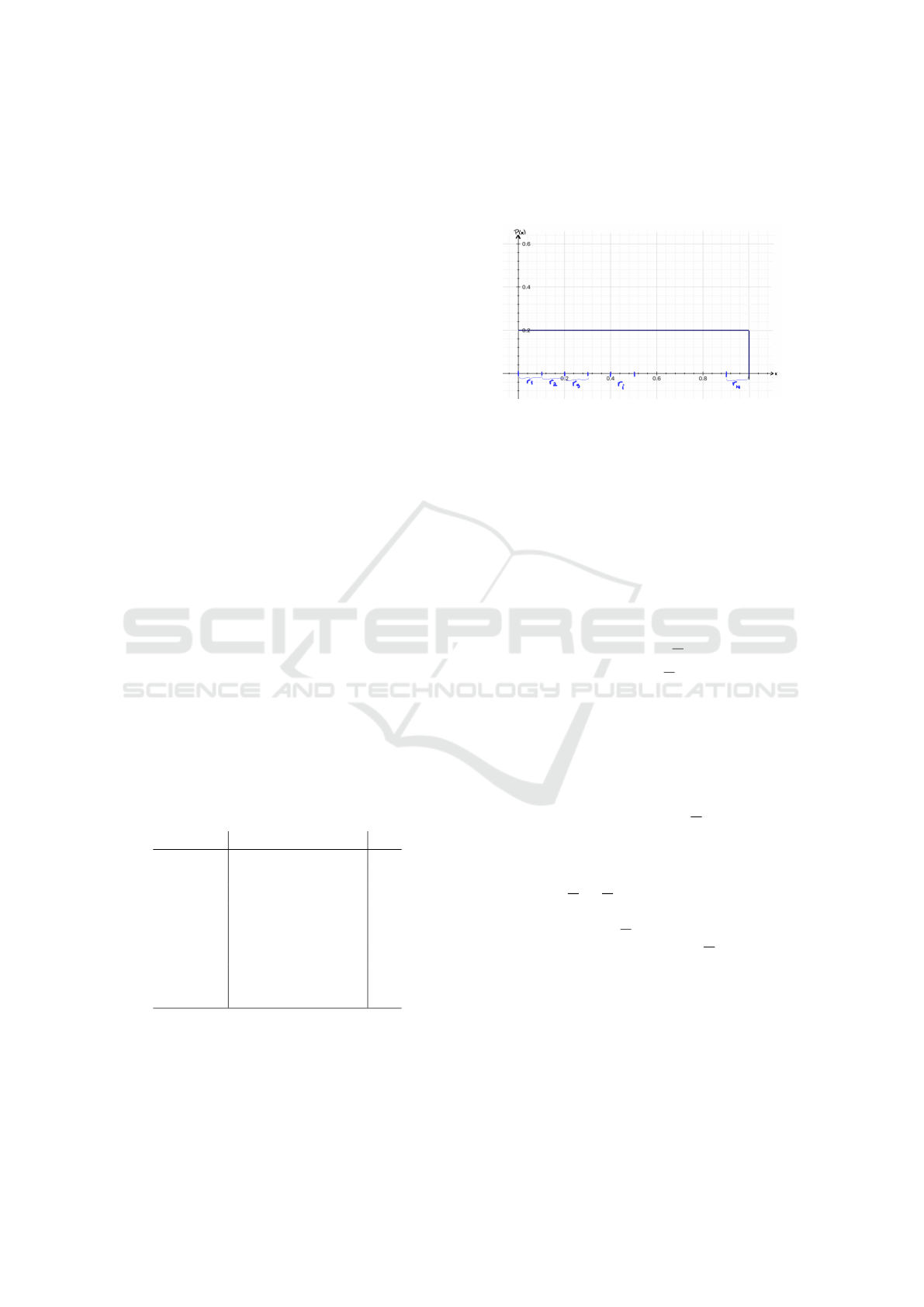
bilities is created, as it is shown in Table 4.

Table 4: Symbol output range table.

Output i Range r

0 [0,c

ji,1

) r

1 [c

ji,1

+ c

ji,2

) r

... ... ...

k [

k−1

∑

m=1

ji,m

∑

m=1

ji,m

) r

... ... ...

K-1 [

K−1

∑

m=1

ji,m

,1] r

A random number x with uniform density between 0

and 1 is generated and using Table 4 it is checked in

which range this number is, if r

≤ x < r

i+1

then the

ﬁrst state output is AC

= U

i f 0 ≤ x < r

the output 0 is generated, that is Stop

i f r

≤ x < r

k+1

the output k is generated

This procedure continues for t > 1 with:

( j) = max

1<i<N

[δ

t−1

(i)a

i j

), 1 < j < N (8)

= j = arg max

1<i<N

[δ

(i)]

And generating AC

in the same way as it was de-

scribed before.

Summarizing for execution of robots’ behaviors

using EHMMs:

INPUTS:

EHMM λ = (A,B,C,π)

Robot’s initial pose: X

= (x

)

Robot’s ﬁnal pose: X

= (x

)

OUTPUTS:

Robot’s actions: AC = { stop, forward,

backward, turn left (45

◦

), turn right (−45

◦

), turn left

and go forward, turn right and go forward and turn

right twice (−90

◦

) and go forward}

t = 1

= quantized sensor data in X

(i) = π

), 1 < i < N,

= j = arg max

1<i<N

[δ

(i)]

= Action(S

,C)

WHILE {X

6= X

}

t = t + 1

= Movement(X

t−1

,AC

t−1

)

= quantized sensor data in X

( j) = max

1<i<N

P[S

...S

t−1

= i, O

,...,O

|λ],

1 < j < N

= j = arg max

1<i<N

[δ

(i)]

= Action(S

,C)

ENDWHILE

The robot’s behavior with a PFSM using a model

EHMM λ = (A, B,C,π) can be optimized by several

methods: Waum-Welch, Genetic Algorithms, etc. In

our research, we optimized the model using GA.

Generating Reactive Robots’ Behaviors using Genetic Algorithms

703

5.5 Range Quantizer

In our research a range vector quantizer is used, which

has N range centroids vectors that best represent the

majority of the sensor readings. To create the range

quantizer ﬁrst the robot collects range vectors.

= (r

,...,r

)

Each r

represents distance from the range sensor to

the objects in line of sight at time t.

The robot navigates in the environment to collect

range vectors by taking readings with its range sen-

sors:

= (r

,...,r

)

= (r

,...,r

)

...

= (r

,...,r

)

Given a set of N

vectors of range readings, a set

of centroids C = (C

,...,C

) that best represent

them, is found using the vector quantization Lloyd’s

algorithm called LBG (Linde-Buzo-Gray).

The robot gets a reading with the range sensor, ob-

taining a range vector S

and to quantize it, it is com-

pared with each of the centroids of the range quantizer

C. And it is choose the centroid vector C

, that is the

closest vector to it.

The centroid C

is chosen if:

d(S

) < d(S

) ∀ j

d(S

)

is a function that measures the similitude of the vec-

tors S

and the C vectors of the quantizer.

In this case the similitude function uses the Eu-

clidean distance. For our experiments we use 8 range

centroids.

The orientation of the light source relative to the

robot is quantized with 8 quadrants.

Also the intensity of the light source is quantized

in 4 values.

6 EVOLUTIONARY ROBOTICS

Evolutionary Robotics (ER) refers to the ﬁeld of in-

quiry comprising methods for automatically generat-

ing artiﬁcial brains and morphologies for autonomous

robots that are inspired by Darwinian evolutionary

theory (Floreano et al., 2008). Some applications

of ER include (Konig, 2015): (i) obstacle avoid-

ance (Banzhaf et al., 1997; Seok et al., 2000; Nelson

et al., 2009), (ii) wall following (Banzhaf et al., 1997),

(iii) object seeking (Banzhaf et al., 1997), (iv) active

vision (Marocco and Floreano, 2002), and (v) object

detection.

Our research is concentrated on how to evolve

robots algorithms for object seeking and obstacle

avoidance using the concept of deterministic and

probabilistic state machines. To achieve this goal

FSM and Extended Hidden Markov Models (EHMM)

robot’s behavior model, λ = (A,B,C,π), are evolved

to ﬁnd individuals that are able to look for light source

beacon while avoiding obstacles using Genetic Algo-

rithms.

A GA performs operations over populations of so-

lutions that resemble sexual reproduction, mutation

and artiﬁcial selection of apt individuals in a given en-

vironment. Often classiﬁed within the realm of search

and optimization algorithms, it has been argued they

are robust techniques that trade off efﬁcacy and efﬁ-

ciency when dealing with different environments by

exploiting intrinsic parallelism. The population dy-

namics allows for the emergent convergence to spe-

ciﬁc regions of the search space as well as implicit

clustering of solutions. Genetic algorithms have been

successfully applied to a variety of engineering and

scientiﬁc problems. In particular to the evolution of

robot controllers and behaviors.

1. First a population is generated randomly, with L

individuals B

,...,B

, in which each individual’s

chromosome is a string of binary numbers that repre-

sents the behaviors B

= {011011...0101}.

The string is separated into small segments that

represent the parameters that deﬁne the behavior, B

{bh

... bh

2. Each individual (chromosome) is evaluated giv-

ing a ﬁtness value according to the individual’s per-

formance. The ﬁtness function evaluates how well the

robot’s behavior performed his operation, and it takes

into consideration several aspects of its performance.

Some of them are: the distance between the last

position reached and the goal, the number of times

the robot hits an obstacle, the number of steps used to

reach the goal and also the number of times the robot

went backward, etc.

The Fitness function used in our experiments is:

Fitness = K1 ∗ N ∗ D

+ K2 ∗ N/D

+ K3 ∗ S

The mobile robots have N

discrete times to go from

an origin to a destination. N

is the number of steps of

that the robot used to reach a destination. If the robot

did not reach the destination N

= N

For the ﬁrst term of the Fitness function, N =

− N

+ 1)

is the distance between the last position of the

robot X and the robot’s original position X

: D

ICAART 2021 - 13th International Conference on Agents and Artiﬁcial Intelligence

704

kX − X

k, that means that a robot that uses few steps

to reach the destination and it gets faraway from its

original position will be well evaluated.

For the second term D

is the distance between the

last position of the robot and the destination goal, plus

distance of to the destination using the shortest path

found by the Dijkstra algorithm in a topological map

of the environment. This is to make the robot to learn

that even that is closed to an obstacle, but if there is an

obstacle in front of it, it needs to surround the obsta-

cle. The Dijkstra algorithm is only used for training,

when the ﬁnal behavior is obtained, is no longer used

by the robot navigation system.

= kX − X

k + DistDi jkstra(X ,X

)

DistDijkstra (X, X

) is a function that measures the

distance of the nodes of a topological that joins the

last position of the robot X and the destination posi-

tion X

using the Dijkstra algorithm. Dividing N by

makes this function to reward individuals that get

closed to the destination.

The third term of the Fitness function is the stan-

dard deviation σ, S

, of the robot’s positions X

be-

tween the robot’s original position X

and its ﬁnal po-

sition X. This term is to measure if the robot went

into a local minimum.

Constants K

and K

are used to tone the per-

formance of the robot according to its speciﬁcations.

The value of the constants Ks where found empiri-

cally: K

= 10, K

= 20 and K

= 11.

3. Select the best individuals according to their ﬁt-

ness function and create a new population with indi-

viduals generated trough evolutionary’s operators (se-

lection, crossover and mutation).

4. The offspring and their selected parents form

the new population.

5. Iteration from 2 to 4 is repeated for M genera-

tions or until the overall ﬁtness criteria between two

generation is less than a given ε, or total number of

generations N

is achieved.

• Evolving Robot Behaviors using Potential Fields.

For the potential ﬁeld approach we evolved some of

the constants of this behavior: η, ε

and d

Each of these constants where represented by 16

bits, 1 bit for the sign, 7 bits for the integer part and

8 bits for the fraction one. Thus, each individual was

represented by 48 bits, and the population consist of

100 individuals. This requires 48 bits per individual’s

chromosome.

• Evolving FSM Behaviors.

The algorithm of the FSM was implemented using the

concept described before of building state machines

using memories or look-up tables, as is shown in Fig-

ure 2. Each Evolved Finite State Machines (EFSM)

had 16 states (4 bits). The inputs of the sensors are

structurated in the following way: 16 range values are

introduced in a range vector quantizer with eight cen-

troids, with the index of the closest centroid, the quan-

tized quadrant index and the quantized light source,

they are concatenated to form the input. This input

is concatenated with the next state to form the next

state index for the look-up table. Thus this index is

formed by concatenating 2 bits of the quantized light

source, 3 bits of the quantized orientation, 3 bits of

the index of the range VQ and 4 bits that represent

the next state, in total giving 12 bits. Then the size of

the look-up table is 4096 rows of a size of 7 bits each,

4 bits that represent next state and 3 bits to indicate

the output. This requires 28672 bits per individual’s

chromosome.

• Evolving EHMM Behaviors.

The extended HMM requires to ﬁnd each of the com-

ponents of its model λ = (A,B,C, π). For the EHMM

behaviors we deﬁned each individual chromosome as

follows: number of states N

= 16, number of obser-

vation symbols N

= 256, number of outputs N

= 8,

and the number of bits per variable N

= 8.

Then, there are N

probabilities variables for vec-

tor π, N

for matrix A, N

for matrix B and

for matrix C. In total the number of bits per

individual is

= N

+ N

= 8x(16 + 16x16 + 16x256 + (16x256)x8) =

297,088

7 EXPERIMENTS AND RESULTS

We tested the behaviors using our simulation module,

in which range readings to obstacles can be simulated,

as well as, the robot’s movements. The simulated mo-

bile robot had a 240 degree simulated range readings,

as the laser Hokuyo URG

04LXUG01, selecting the

readings with a separation of 15 degrees each, making

16 range readings in each sensing.

The destination goal is described by a yellow cir-

cle; the free space is green; the obstacles are described

by polygons in red; the robot is a black circle and the

proximity sensor readings are represented by blue col-

ors.

For the genetic algorithm, we had a population of

100 individuals and the evolution lasted 900 gener-

ations. The robot’s radio was r = 3cm. During the

Generating Reactive Robots’ Behaviors using Genetic Algorithms

705

execution of the GA, noise was added to the move-

ments of the robot, as well as, to the sensors: for the

linear movement it was added a random variable with

a uniform density function of [−0.004,0.004] meters,

for rotation movement a uniform density function of

[−0.03927,0.03927] radians and for the range sen-

sor a Gaussian random variable with mean µ = .004

and standard deviation σ = .0004. The behaviors,

to avoid obstacles, were tested in 13 simulated envi-

ronments, with different sizes, conﬁgurations, robot’s

starting positions and goal destinations. There were

two types of environments: one with random gener-

ated polygons; and ofﬁce type environments, similar

to the shown in ﬁgures 5 and 6

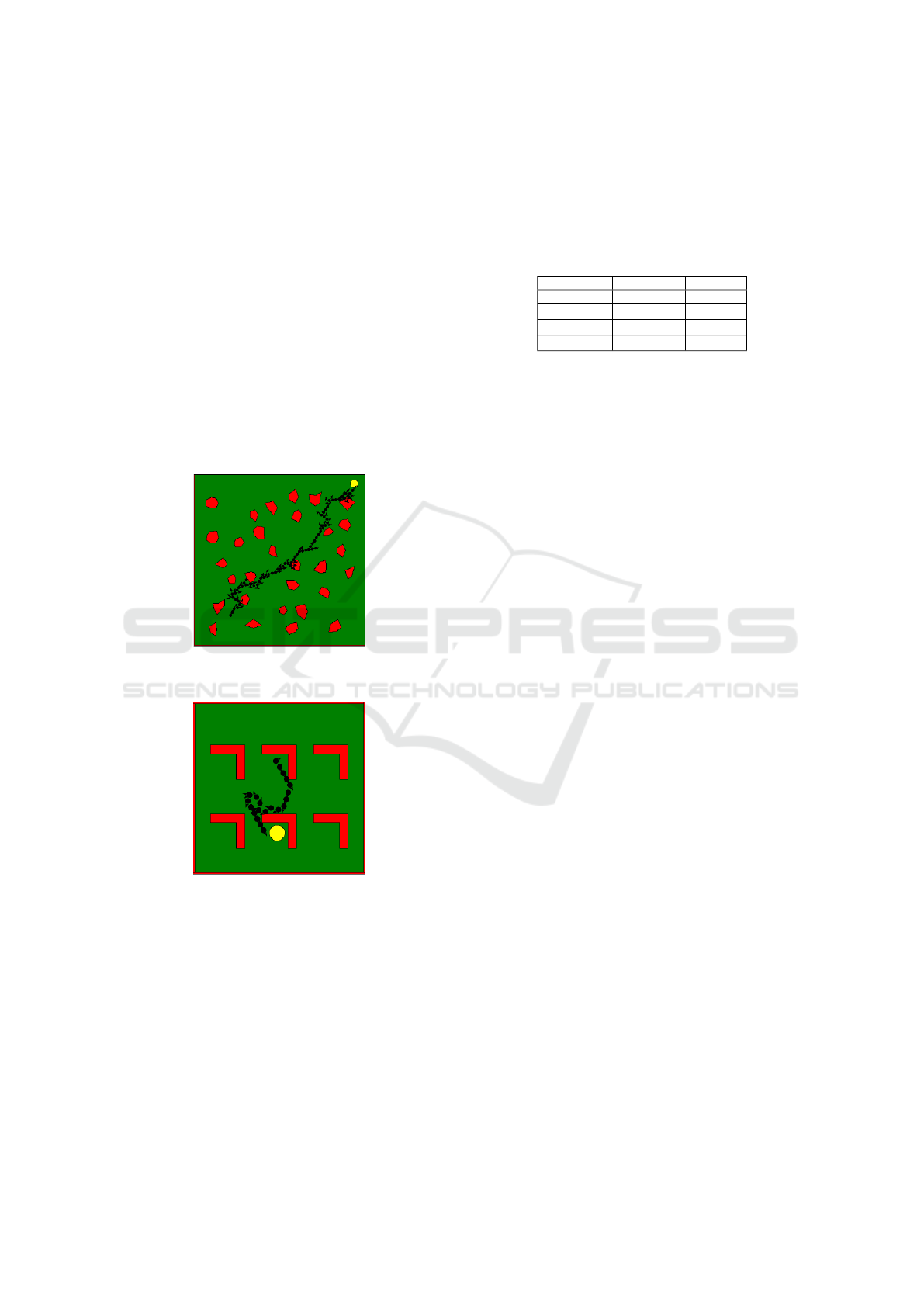
The Figures 5 and 6 show evolved behaviors with

a robot starting in a initial position and reaching a des-

tination, a light source, in two types of environments.

Figure 5: The path found by an evolved robot’s behavior in

a polygon type environment.

Figure 6: The path found by an evolved robot’s behavior in

a ofﬁce type environment.

Table 5 shows the average performance of the best

individuals for each of the behaviors in polygon and

ofﬁce type environments, during 1000 trials. As we

can see in both cases the best performance is done by

the FSM behavior.

Despite the fact that all the behaviors performed

worst in the ofﬁce type environments, we can see

that in this type of environments the performance

of the behaviors with memory, the FSM and PFSM

are much better than the potential ﬁeld behavior ap-

proach, that does not have any memory. In polygonal

type environments the FSM is better than the potential

ﬁeld approach by 14.8 % and for ofﬁce type environ-

ments is by 21.94 %.

Table 5: Best average ﬁtness of the behaviors in two differ-

ent type environments: Polygons and Ofﬁce.

Env. Polygons Env. Ofﬁce

Behavior Fitness Fitness

FSM 4267 2541

PFSM 4243 2153

POTENTIALS 3635 1983

8 CONCLUSIONS

We proposed the optimization of the methods for po-

tential ﬁelds and state machines to achieve mobile

robot behaviors, the state machines were built us-

ing deterministic and probabilistic methods. For the

deterministic FSM we proposed an architecture of a

state machine that uses a look-up table that encodes

the algorithm, that is, the robot behavior. This look-

up table contains the next state and the outputs of each

state. The inputs of the state machine, sensors, and

the next state are linked together to form the index

of the look-up table that contains the next state and

outputs for the present state. For the PFSM a modi-

ﬁed version of Hidden Markov Models, that we called

EHMM, was used to encode the mobile robot behav-

ior. We also proposed how to ﬁnd the optimum be-

haviors for potential ﬁeld approach, the FSM and the

PFSM using Genetic Algorithms. Our experiments

proved that the obtained robots’ behaviors, when they

are used for robot navigation, that the deterministic

FSM outperforms the potential ﬁeld approach and the

PFSM.

The robot’s behaviors using FSMs and the PFSMs

outperforms the ones using potential ﬁelds, mainly

because they are more complex machines and they are

able to stay out of local minima and can retain some

memory and learn how to get out of these. Meanwhile

the FSM outperforms the PFSMs behaviors due to

the type of environments where the experiments were

tested and the type of noise that was added to the sen-

sory data, as well as, to the robot’s movements. For

future work it is necessary to test with more strong

noise and more complex HMMs, with more states and

observation symbols to see if their performance im-

proves.

ICAART 2021 - 13th International Conference on Agents and Artiﬁcial Intelligence

706

REFERENCES

Arkin, R. (1998). Behavior-Based Robotics. MIT Press.

Cambridge. MA 1998.

Banzhaf, W., Nordin, P., and Olmer, M. (1997). Generating

adaptive behavior using function regression within ge-

netic programming and a real robot. In Proceedings of

the Second International Conference on Genetic Pro-

gramming, San Francisco, pages 35–43.

Barricelli, N. A. (1954). Esempi numerici di processi di

evoluzione. volume 6, pages 45–68. Methods.

Brooks, R. (1986). A robust layered control system for a

mobile robot. In IEEE Journal of Robotics and Au-

tomation, volume 2, pages 14–23. IEEE.

Floreano, D., Husbands, P., and Nolﬁ, S. (2008). Evolution-

ary robotics. In Springer handbook of robotics, pages

1423–1451. Springer.

Fogel, D. B. (2006). Nils barricelli-artiﬁcial life, coevolu-

tion, self-adaptation. In Computational Intelligence

Magazine, volume 1, pages 41–45. IEEE.

Fraundorfer, F. and Scaramuzza, D. (2012). Visual odome-

try [tutorial]. In IEEE Robotics and Automation Mag-

azine, volume 19, pages 78–90. IEEE.

Guo, R., Sun, P., Lindgren, E., Geng, Q., Simcha, D.,

Chern, F., and Kumar, S. (2020). Accelerating large-

scale inference with anisotropic vector quantization.

Konig, L. (2015). In Complex Behavior in Evolutionary

Robotics. Walter de Gruyter GmbH & Co KG, 2015.

Latombe, J.-C., Lazanas, A., and Shekhar, S. (1991). Robot

motion planning with uncertainty in control and sens-

ing. Artiﬁcial Intelligence, 52(1):1 – 47.

Marocco, D. and Floreano, D. (2002). Active vision and

feature selection in evolutionary behavioral systems.

In From animals to animats, volume 7, pages 247–

255.

Mohanan, M. G. and Salgaonkar, A. (2020). Probabilistic

Approach to Robot Motion Planning in Dynamic En-

vironments. SN Computer Science, 1(181).

Negrete, M., Savage, J., and Contreras, L. (2018). A

Motion-Planning System for a Domestic Service

Robot. SPIIRAS Proceedings, 60(5):5–38.

Nelson, A. L., Barlow, G. J., and Doitsidis, L. (2009). Fit-

ness functions in evolutionary robotics: A survey and

analysis. volume 57, pages 345–370. Elsevier.

Rabiner, L. and Juang, B. (1986). An introduction to hidden

markov models. volume 3, pages 4–16. Assp maga-

zine, IEEE.

Savage, J., Fuentes, O., Contreras, L., and Negrete, M.

(2018). Map representation using hidden markov

models for mobile robot localization. In 13th Interna-

tional Scientiﬁc-Technical Conference on Electrome-

chanics and Robotics.

Seok, H.-S., Lee, K.-J., and Zhang, B.-T. (2000). An on-

line learning method for objectlocating robots using

genetic programming on evolvable hardware. In Pro-

ceedings of the Fifth International Symposium on Ar-

tiﬁcial Life and Robotics, volume 1, pages 321–324.

Citeseer.

Shahriar, S. and Zelinsky, A. (1999). Mobile robot naviga-

tion based on localisation using hidden markov mod-

els. In Australasian Conference on Robotics.

Shahriar, S. and Zelinsky, A. (2014). Robot localization

from minimalist inertial data using a hidden markov

model. In IEEE International Conference on Au-

tonomous Robot Systems and Competitions.

Vidal, E. and Thollard, F. (2005). Probabilistic ﬁnite-state

machines. In IEEE Transactions on Pattern Analy-

sis and Machine Intelligence, volume 27, pages 1013–

1025.

Viterbi, A. (1967). Error bounds for convolutional codes

and an asymptotically optimum decoding algorithm.

In IEEE Transactions on Information Theory, vol-

ume 13, pages 260–269.

Yakoubi, M. A. and Laskri, M. T. (2016). The path planning

of cleaner robot for coverage region using genetic al-

gorithms. In Journal of Innovation in Digital Ecosys-

tems, volume 3.

Yakoubi, M. A. and Laskri, M. T. (2018). Genetic algo-

rithm based approach for autonomous mobile robot

path plannings, procedia computer science. 127:180–

189.

Generating Reactive Robots’ Behaviors using Genetic Algorithms

707