Deep Convolutional Second Generation Curvelet Transform-based MR

Image for Early Detection of Alzheimer’s Disease

Takrouni Wiem

and Douik Ali

University of Sousse, ISITCom, 4011, Sousse, Tunisia, Networked Objects Control and Communication Systems

Laboratory (NOCCS-ENISO), 4054, Sousse, Tunisia

University of Sousse, ENISO, Networked Objects Control and Communication Systems Laboratory (NOCCS),

Keywords:

Second-Generation Curvelet (SGC), Mild Cognitive Impairment (MCI), Multiclass Classiﬁcation.

Abstract:

Merging neuroimaging data with machine learning has an important potential for the early diagnosis of

Alzheimer’s Disease (AD) and Mild Cognitive Impairment (MCI). The applicability of multiclass classiﬁ-

cation and the prediction to deﬁne the progress of different stages of the disease have been relatively under-

studied. This paper presents a short review of the deep learning history and introduces a new solution for

delineating changes in each stage of AD. Our Deep Convolutional Second-Generation Curvelet Transform

Network (SGCTN) is divided into both levels: The feature learning level is the ﬁrst task that can combine a

Second-Generation Curvelet (SGC) with autoencoder trained features. Then, for each hidden layer, a pool-

ing is used to obtain our convolutional neural network. This network is used to learn predictive information

for binary and multiclass classiﬁcation. Our experiments test uses a different number of Cognitively Normal

(CN), AD, early EMCI, and Later LMCI subjects from the AD Neuroimaging Initiative (ADNI). Magnetic

Resonance Imaging (MRI) information modalities are considered as input. The proposed DSGCCN achieves

98.1% accuracy for delineating the early MCI from CN. Furthermore, for detecting the distinctive level of

AD, a multiclass classiﬁcation test realizes the global accuracy of , and it more particularly differentiates MCI

and AD groups from the CN group with 96% accuracy. Compared to the state-of-the-art deep approach, our

results indicate that our architecture can achieve better performance for the same databases. Model analysis

based (SGC) can improve the classiﬁcation performance via comparison experiments.

1 INTRODUCTION

Recent research by Alzheimer’s Statistics reports that

for Alzheimer’s Disease (AD) in the world, almost

50 million people have Alzheimer’s or related de-

mentia with only one in four people with AD have

been diagnosed. AD and other dementia are the top

reason for disabilities in later life. Seventy-two per-

cent of the projected rise in the global burden of de-

mentia and pervasiveness by 2050 will take place in

low and middle-income countries (Ryu et al., 2017).

AD is neuropathologically identiﬁed by grievous cell

loss and cortical atrophy along with an elevated de-

mentia index as calculated by numbers of neuritic

plaques and neuroﬁbrillary tangles in the hippocam-

pus and the neocortex. This disease gets worse with

time and later declines cognitive functions and behav-

ioral impairments that touch memory, language and

thought, including forgetfulness. Cure strategies for

AD are concentrating on preventing the AD evolu-

tion or speeding up the clearance of these aggregates.

AD, composed of different neurodegenerative levels,

which represent the mutation from one stage to an-

other and identiﬁes each one by the speciﬁcity of the

biomarker. It is indicated that 15-25% of people aged

60 or older have a prodromal stage of AD that can be

related to Mild Cognitive Impairment (MCI), which is

a transitional stage between dementia and the normal

cognitive function. A patient diagnosed with MCI can

either have later MCI (LMCI) or Early MCI (EMCI)

due to age-linked memory degradation, hence the ac-

cent on the importance of early diagnosis of the dis-

ease. Thus, accurate and early diagnosis of MCI can

help path disease progression, supply better treatment

paradigms for patients, and decrease medical costs.

Nevertheless, neuroimaging and clinical studies have

exposed differences between MCI and Cognitively

Normal (CN) (Scheltens and Korf, 2000), (Silverman,

2009). To identify pathological biomarkers to under-

Wiem, T. and Ali, D.

Deep Convolutional Second Generation Curvelet Transform-based MR Image for Early Detection of Alzheimer’s Disease.

DOI: 10.5220/0010228902850292

In Proceedings of the 16th International Joint Conference on Computer Vision, Imaging and Computer Graphics Theory and Applications (VISIGRAPP 2021) - Volume 4: VISAPP, pages

285-292

ISBN: 978-989-758-488-6

285

stand the mechanism causes and monitor early brain

changes for each stage of the disease, the quantitative

prognosis of AD/MCI by analyzing different types of

neuroimaging modalities is necessary for the early

classiﬁcation of AD. Magnetic Resonance Imaging

(MRI) allows measuring spatial patterns of atrophy

and their growth with disease evolution. It also sup-

plies visual information concerning the macroscopic

tissue atrophy, which results from the cellular changes

and detects neuronal injury and degeneration under-

lying AD/MCI (Davatzikos et al., 2011). Positron

Emission Tomography (PET) (Nozadi et al., 2018)

can be used for the examination of the cerebral glu-

cose metabolism which indicates the functional brain

activity. Thereby, a trustworthy diagnosis from brain

modalities is necessary, and a sturdy Computer-Aided

Diagnosis (CAD) by the data anatomization of neu-

roimaging will enable for a more reliable and infor-

mative approach and can increase potentially diag-

nostic accuracy. A classical interpretation process for

exploring biomarkers for the neuropsychiatric analy-

sis disorders has been founded on the univariate mass

statistics within the assumption that various regions

of the brain act independently. Nevertheless, this as-

sumption (Fox et al., 2005) is not suitably speciﬁed

for our present comprehensive brain functioning.

2 RELATED WORK

Machine Learning (ML) methods, which can lay hold

of the correlation between regions into account, have

become the basic integration and attraction of CAD

techniques (Davatzikos et al., 2008), (Suk et al., 2017)

and have been broadly used for the automated diag-

nosis and interpretation of brain disorders. Further-

more, various ML classiﬁcation models have been

used to develop automated neurological disorder pre-

diction. Both major research orientations include

Support Vector Machine (SVM) (Pinaya et al., 2016)

and Deep Learning (DL) based diagnostic models

(Greenspan et al., 2016), (Litjens et al., 2017). SVM-

based models of brain disorders have been criticized

for their poor performance on raw data and for re-

quiring the expert use of design techniques to ex-

tract informative handcrafted features. In contrast,

DL models enable a system to use raw data as in-

put, thus allowing them to automatically ﬁnd highly

discriminating features in the training dataset (Shen

et al., 2017). As a recent successful category of unsu-

pervised learning models, autoencoders, such as con-

volutional (Masci et al., 2011), variational (Kingma

and Welling, 2013), k-sparse (Makhzani and Frey,

2013), contractive (Rifai et al., 2011) and denois-

ing ones (Vincent et al., 2008), perform an impor-

tant role in feature extraction, dimension reduction

and generative tasks. Higher data dimensionality is

an endemic characteristic of medical data, and learn-

ing efﬁcient coding for image classiﬁcation is the

goal of these autoencoders. It is crucial to note that

these approaches distort spatial locality (neighbor re-

lations) in brain-imaging data (Suk et al., 2017), (Liu

et al., 2019), (Payan and Montana, 2015) over the fea-

ture extraction level. Many automated systems have

been developed in the last years for binary classi-

ﬁcation (normal or abnormal) of brain MRI, which

have made remarkable progress. However, multi-

class classiﬁcation into a speciﬁc grade of brain dis-

eases is comparatively more challenging and has great

clinical signiﬁcance. Numerous methods have been

utilized to analyze using the wavelet or its variants

to extract features for the task of binary and multi-

class brain MRI, despite their defeat to capture direc-

tional features at numerous levels of resolution (Gudi-

gar et al., 2019), (Jia et al., 2019), (Nayak et al.,

2017). In the last mentioned references, the em-

ployed classiﬁers, like the SVM, the fuzzy neural net-

work, and Least-squares SVM endure critical issues

such as high computational complexity, poor scala-

bility and slow learning speed. In (Zhang and Sug-

anthan, 2016), the random vector functional link net-

work was a classiﬁer that afforded great generaliza-

tion performance at the speed learning property. The

hybrid approach (Gao et al., 2018) combined the MRI

texture features of the contourlet-based hippocampal,

the regional CMgl measurement based on ﬂuorine-

18 ﬂuorodeoxyglucose-positron emission tomogra-

phy, medical history, the morphometric volume, the

neuropsychological tests of symptoms with the multi-

variant models to enhance the AD classiﬁcation and

the prediction of MCI conversion, and to appraise

whether the partial least squares and the Gaussian

process were realizable in developing multivariate

models in such a situation. Hence, this situation had

various limitations, only hippocampal MRI texture

features were explored, the size was approximately

modest, and the power statistical might be restricted.

Thus, this model was insensitive to high-dimensional

data, and dimensionality reduction might upgrade the

predictive achievement of this model. However, very

few studies have been announced up to now concern-

ing multiclass AD classiﬁcation, predicting MCI con-

version and precision detection. Even more, it re-

mains unknown which method is more appropriate

for processing high-dimensional data in this context.

To address the above problems, in the present study,

we propose a new combination of a Second Genera-

tion Curvelet Transform Network (SGCTN) and Deep

VISAPP 2021 - 16th International Conference on Computer Vision Theory and Applications

286

Convolutional Autoencoder (DCA) for early detec-

tion of AD and prediction of MCI conversion. A DCA

consists of operating the classiﬁcation of a particu-

lar class against all the other classes of the dataset by

the reconstruction of Deep Convolutional (SGCTN).

This reconstruction is achieved using a sequence of

a stacked autoencoder and a linear classiﬁer. The re-

maining part of this paper is composed of four sec-

tions. The Deep Convolutional (SGCTN) is proposed

in section III. An overview of the dataset utilized in

the classiﬁcation test is given in section IV. Section V

includes the experiments and the results of the test.

Finally, Section VI summarizes and concludes this

paper.

3 PROPOSED DEEP

CONVOLUTIONAL (SGCTN)

To improve the rate of convergence and classiﬁcation

performance, a new approach called Deep Convolu-

tional (SGCTN) is constructed. In this section, we

describe the theoretical background steps that lead to

our approach.

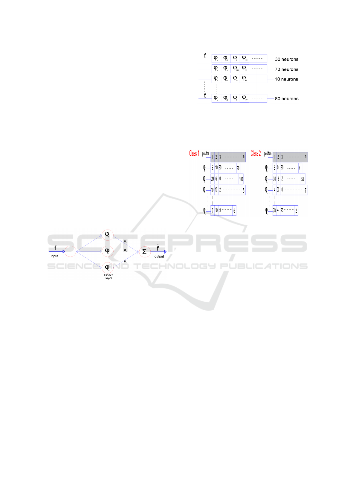
Figure 1: The SGCTN for one element of class.

• Step 1: We construct the SGCTN for each object

of a class using the best algorithm (Dubois et al.,

2015), (Ma and Plonka, 2010). Figure 1 is consti-

tuted for three layers. The SGCTN is deﬁned by a

much simpler and more natural indexing structure

with three parameters: scale, orientation (angle)

and location, so curved singularities can be well

approximated with very few coefﬁcients and in a

non-adaptive manner. We deﬁne an SGCTN by

pondering a series of second generation curvelets

(SGC) interpreted and widened from one mother

SGC atom with weight values to approximate a

determined signal f:

f =

∑

i=1

) (1)

• Step 2: Every SGCTN is shown in the form of a

table (Figure 2). The neuron number that contains

a SGC can vary for each SGCTN created in step

Figure 2: Tables of each SGCTN for a class.

• Step 3: In this stage, we select the best SGC (cho-

sen in step 2) to produce an SGCTN for a class.

Thereby, we account that our brain dataset is com-

posed of two classes:

Figure 3: Tables of the number of appearance of each SGC

for a class.

- Class 1 which we will represent in a SGCTN.

- Class 2 which includes all the other classes of

the dataset.

We build tables for all the SGC in the dataset of

SGC for the two classes (Class 1 and Class 2).

The tables hold the number of emergences of each

SGC in each position in all the SGCTN utilizing

the tables in step 2 (Figure 3). Subsequently, we

calculate a coefﬁcient for every SGC in that man-

ner: for ϕ

in class 1, the coefﬁcient is determined

by the sum of all the values of ϕ

that are multi-

plied by (1+ (n - i)) in each position (i) and the

identical operation is used for ϕ

in class 2. This

is indicated as follows

Class1

coe f

=Class2

coe f

∑

i=1

∗(1+(n−i)))

(2)

Whence, the global coefﬁcient for ϕ

is deﬁned as

follows

Glob

coe f

= Class1

coe f

−Class2

coe f

(3)

Next, we calculate all global coefﬁcients of all

SGC and arrange them on a table ordered from the

biggest to the smallest (Figure 4). The method of

coefﬁcient calculation for all SGC enables penal-

izing the SGC frequently utilized in other classes

(in our instance, the classes are combined in one

class: class 2) and the preferred SGC used in the

Deep Convolutional Second Generation Curvelet Transform-based MR Image for Early Detection of Alzheimer’s Disease

287

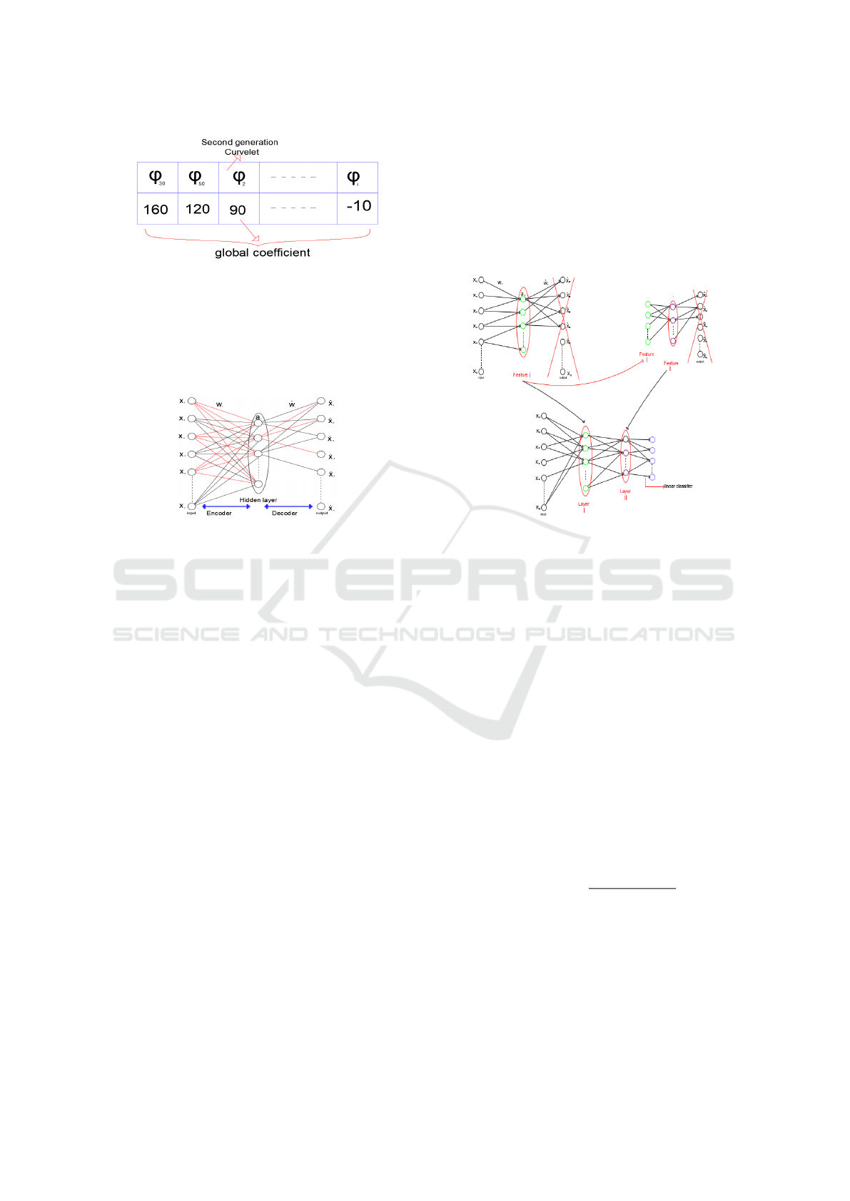
Figure 4: Tables of the global coefﬁcient for each SGC.

working class (Class1). For example, if ϕ

is the

ideal SGC utilized in class 1 in the ﬁrst position

with 30 emergences and the ideal SGC in class 2

in the second position with 200 emergences, we

calculate the ϕ

coefﬁcient to punish it and avert it

in the ﬁrst position.

Figure 5: SGCTN for a class.

• Step 4: We construct a novel SGCTN for a class

(Figure 5) utilizing the ideal SGC from the table in

step 3. The total of the SGC utilized for the overall

SGCTN is the average of the SGC numbers used

in step 2.

• Step 5: In this stage, we construct a network (with

the use of the SGC in our SGCTN that produces

a class in step 4) using an autoencoder algorithm.

It is important to note that an encoder level gener-

ates a feature vector (hidden layer) from the input

vector with a primal SGC and a decoder level that

reconstructs the input vector from the vector of a

feature with a dual SGC. In this phase, the neurons

of the hidden layer incorporate a linear function.

We take into consideration that:

f = x

, x

, ..., x

f = ˆx

, ˆx

, ..., ˆx

= w

, w

, ..., w

= ˆw

, ˆw

, ..., ˆw

(4)

Then,

=≺ f , ϕ

=⇒ a

∑

j=1

) (5)

ˆx

∑

j=1

ˆw

(6)

• Step 6: The hidden layer is used to construct our

SGCTN and it is considered for the second train-

ing of the input layer. The hidden layer is used to

construct our deep convolutional SGCTN and it

is considered for the second training of the input

layer. The construction of an SGCTN with both

hidden layers and a linear classiﬁer is displayed

in Figure 6. This process is enforced for all ele-

Figure 6: A deep SGCTN with both hidden layers.

ments of a class until the creation of our deep con-

volutional SGCTN, which ﬁgures the entire class.

After that, we replace the linear function by the

sigmoid function in the hidden layers to enforce

ﬁne-tuning. The choice of using the sigmoid func-

tion is to promote the signiﬁcant features and to

derivate an activation function in the backpropa-

gation step. A few new components are shown

to be very effective when connected to a convolu-

tional neural network:

*Local Contrast Normalization (LCN): This com-

ponent is an efﬁcient technique that makes a

deep architecture more sturdy to illumination

changes that have not been seen under training.

It adapts local subtractive and divisive normaliza-

tions, which impose a kind of local competition

between features at the identical spatial position

in various feature maps and adjacent features in a

feature map. It is determined by this function:

i+1,x,y

i,x,y

− m

i,N(x,y)

(7)

*Geometric Lp-norm Pooling (GLP): Pooling is

the reducing step of spatial resolution, which ag-

gregates local features over the region of inter-

est into a statistic through a certain spatial pool-

ing operation. The GLP method can preserve

the speciﬁc-class spatial/geometric information

on the pooled features and appreciably boosts the

VISAPP 2021 - 16th International Conference on Computer Vision Theory and Applications

288

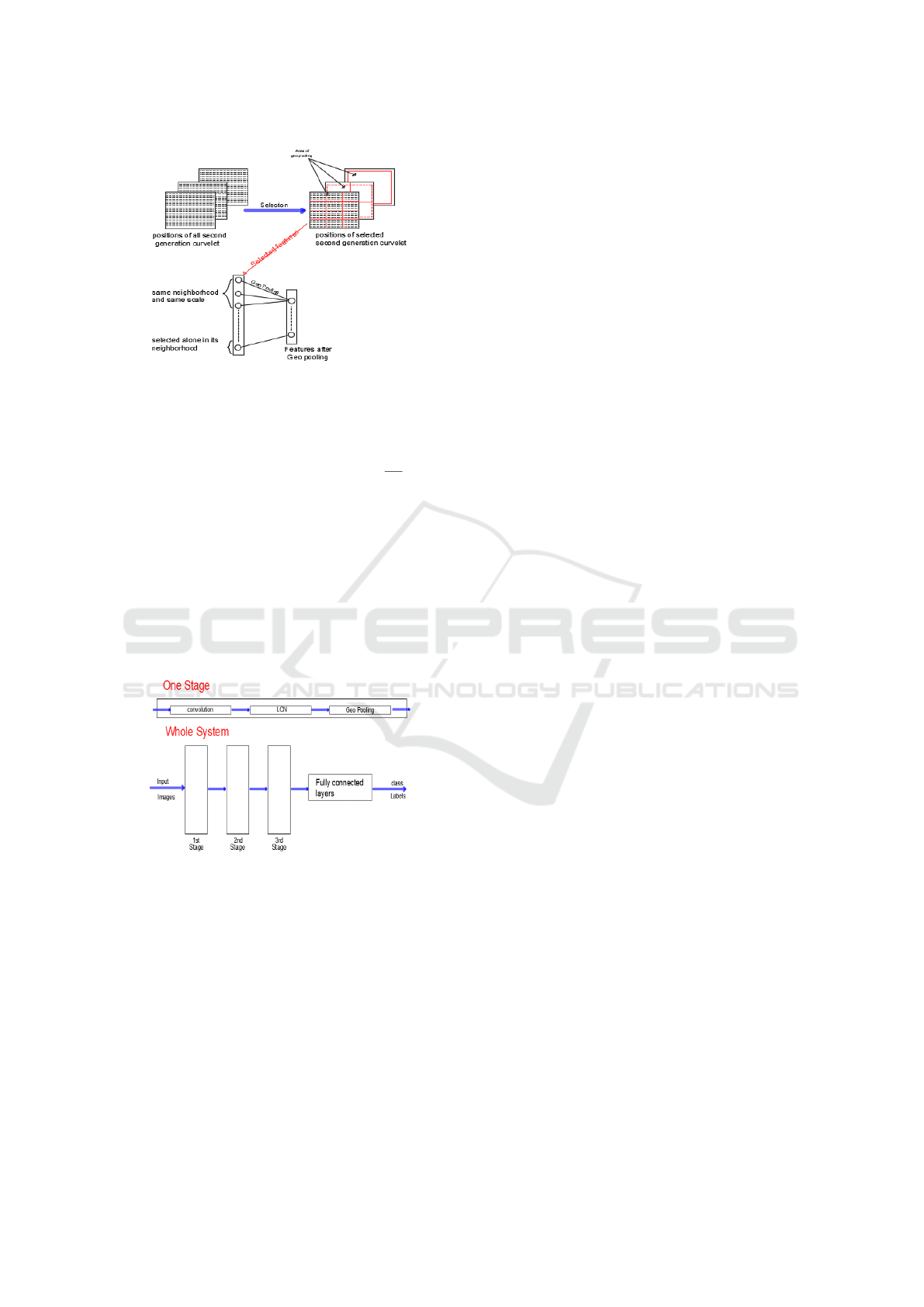
Figure 7: Geometric Lp-norm pooling of adjacent SGC.

discriminating ability of the resultant features for

image classiﬁcation. It is determined by this func-

tion:

Out = (

∑∑

I(i, j)

GLP

∗ G

(i, j))

GLP

(8)

where I is the input feature map, Gk is a Gaus-

sian kernel, and Out is the output feature map. In

our contribution, we achieve intelligence pooling.

We operate it if and only if the SGC that are dis-

covered in the neurons are adjacent, whether of an

identical type or an identical scale (Figure 7). For

that reason, for each hidden layer, GLP and LCN

are employed of our SGCTN and will be consid-

ered as one step (Figure 8). In addition, our deep

convolutional SGCTN will be created.

Figure 8: Typical architecture of Deep convolutional

SGCTN.

• Step 7: For the last stage, a linear weak classiﬁer

is applied, which is deﬁned to be a classiﬁer that

is only slightly correlated with true classiﬁcation.

It plainly classiﬁes data with a unique threshold

on a certain data dimension.

4 DATASET OVERVIEW

In this work, we use the ADNI http://adni.loni.

usc.edu/ dataset including various phases (ADNI-1,

ADNI-2, and ADNI-GO) which is preprocessed by

Freesurfer (v5.3). The ADNI has gathered 1167 scans

of adults aged between 55 and 90, composed of cog-

nitively normal older persons, individuals with early

AD, and individuals with early or late MCI. The

demographic details of subjects are provided in Ta-

ble I. In this paper, we analyze the performance of

our architecture on both T1 and T2 weighted MRI

images collected from the same set of subjects and

evaluate different parameters under both binary and

multi class classiﬁcation. To train our data, parallel

processing is needed, so we use open source pack-

age python 3.0 to perform the training and valida-

tion of the classiﬁer (GPU: 1xTesla K80, having 2496

CUDNN cores, compute 3.7, 24GB(23.439GB Us-

able) GDDR5 VRAM). We use Keras library over

Tensorﬂow modules to design our proposed architec-

ture.

5 EXPERIMENTS AND RESULT

We compare the performance of our model while

training and testing with brain MRI together

with (Original Features Curvelet Network (OFCN),

SGCTN), and segmented hippocampal regions.

5.1 Devising Training and Test Set

We augment the MRI data to resist the model from ge-

ometry changes and noise. We use 5482 MRI slides in

our experiment. We split the data into 85:15 training

and testing sets based on subjects to defeat the intra

relation amid the split data to carry out the classiﬁca-

tion without biasing.

5.2 Classiﬁcation Results and

Discussion

The focus of this work is established on demonstrat-

ing how the proposed approach can resolve the most

discriminating elements related to the progression of

MCI and ameliorate binary and multiclass classiﬁca-

tion performance. After the selection of features, we

train the initial SGCTN to learn the fundamental vec-

tor of features. Those features are connected to the

other input of the autoencoder to learn secondary fea-

tures in order to discriminate the various levels of the

disease. Our network includes seven hidden layers

and a softmax layer for output. We test the classi-

ﬁcation performance in both cases, which is OFCN

and SGCTN. In this latter, we choose ﬁve scales and

eighteen orientations. The results provide the confu-

sion matrix to perform the quality of our architecture,

Deep Convolutional Second Generation Curvelet Transform-based MR Image for Early Detection of Alzheimer’s Disease

289

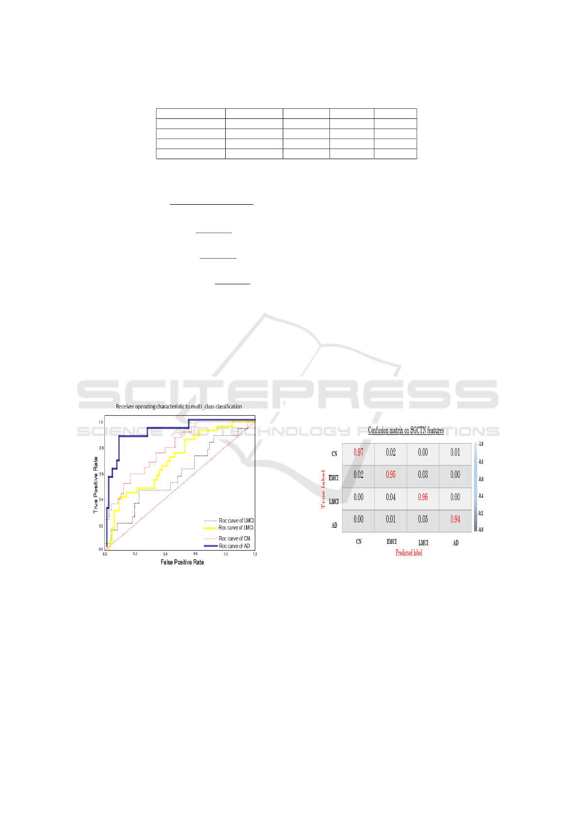
Table 1: Demoghraphic details about the participant study.

Categories Age MMSE CDR CDR GS

AD (284 sc) 75.85 ± 7.94 23.4±2.1 4.5 to 9 0.7±0.3

LMCI (169 sc) 72.99±7.67 27.1± 1.9 2.5 to 4.5 0.5±0.2

EMCI (328 sc) 72.62±7.33 28.4±1.5 0.5 to 2.5 0.5±0.0

Contols (371 sc) 75.68±8.01 29.1±0.9 0 to 0.5 0.0±0.0

which contains actual and predicted class informa-

tion. The following ﬁve metrics are considered:

Accuracy(ACC) =

T P + T N

T P + T N + FP + FN

(9)

Sensitivity(SEN) =

T P

T P + FN

(10)

Speci f icity(SPEC) =

T N

T N + FP

(11)

PositivePredictiveValue(PPV ) =

T P

T P + FP

(12)

Table II proves the results of our network, witch al-

lows distinguishing between CN/AD, CN/EMCI and

EMCI/LMCI. The results are more accurate with

99.1%, 98.1% and 93.3 % in the tasks of CN vs AD,

CN vs EMCI and EMCI vs LMCI, respectively for

the deep convolutional SGCTN using whole image

compared with the OFCN in the same tasks with hip-

pocampal patch are 92.4% 90.8 % and 89.7% is more

accurate than the OFCN using whole image. On the

Figure 9: ROC curves to multiclass classiﬁcation.

other hand, the OFCN model achieves good perfor-

mance in both tasks. This can be explained by the au-

toencoder selecting only each class and separating the

approximation to the components of the other class.

The selection based on the principal contribution of

each best SGC to the construction of the SGCTN for

each component of a class. We note that the SGC

stays unchanged and that the weight changes from

one slide to another for both classes. Then, based on

a SGC, which, in fact includes an extension of the

isotropic multiresolution analysis concept to include

anisotropic scaling and angular dependence (direc-

tionality) while preserving rotational invariance. The

SGC is also faster and less redundant compared to its

original features curvelet (OFC), It does not exhibit

blocking artefacts due to special partitioning.

We use the learning curve of the multiclass

classiﬁcation using the proposed deep convolutional

SGCTN (Figure 9). The classiﬁer can more accu-

rately differentiate CN, AD and LMCI from an EMCI

class, so the overall classiﬁcation performance is ame-

liorated signiﬁcantly. It can be noted that the learning

curve related to the test is closer to the learning curve

of validation. As there are three classes instead of

both classes, the model can learn more generic dis-

criminative elements through all three classes. Then,

the confusion matrix evaluates the performance with

each line corresponding to a true class. The com-

ponents of the diagonal of the confusion matrix de-

pict the point number for the predicted label which

is equal to the true label, whereas the components of

the off-diagonal are those that are misclassiﬁed by the

classiﬁer (Figure 10). Compared with the deep learn-

Figure 10: AD vs. LMCI vs. EMCI vs. CN classiﬁcation

confusion matrix.

ing classiﬁcation model and geometric transform-

based feature extraction pattern analysis based on

ADNI data (Fang et al., 2020), (Wee et al., 2019),

(Ramzan et al., 2020), it should be noted that in Ta-

ble III our proposed architecture still achieves bet-

ter performance in the terms of classiﬁcation accu-

racy for the two tasks (EMCI vs. LMCI and, CN vs.

EMCI). This can be considered for the use of autoen-

coder based SGC, which gives better feature extrac-

tion than other method based on a deep model with

VISAPP 2021 - 16th International Conference on Computer Vision Theory and Applications

290

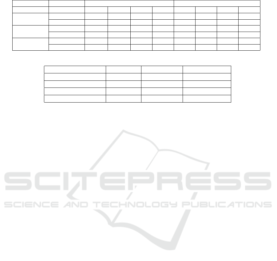
Table 2: Binary classiﬁcation performance comparison of OFCN features and SGCTN features.

Task Features OFCN SGCTN

ACC SEN SPEC PPV ACC SEN SPEC PPV

CN/AD

hippocampal 92.4 % 93.4% 90.2% 90.4% 97.3% 98.3% 96.1% 96.5%

whole slide 91.2% 91.9% 89.9% 90.2% 99.1% 99.8% 98.2% 98.6%

CN/EMCI

hippocampal 90.8% 91.3% 89.3% 89.7% 96.9% 97.2% 95.2% 95.6%

whole slide 90.6% 92.1 % 88.8% 88.9% 98.1% 98.8% 97.2% 97.6%

LMCI/EMCI

hippocampal 89.7% 90.1% 87.9% 88.0% 91.9% 93.2% 90.8% 90.9%

whole slide 86.8% 88.1% 85.8% 85.9% 93.3% 94.5% 92.7% 92.9%

Table 3: Accuracy CN vs. EMCI and EMCI vs. LMCI classiﬁcation comparison.

CN vs. AD CN vs. EMCI EMCI vs. LMCI

(Fang et al., 2020) - 79.25% 83.33%

(Wee et al., 2019) 81.0% - -

(Ramzan et al., 2020) - 96.85% 88.6%

Proposed 99.1% 98.1% 93.3%

or without a transform based on multiresolution anal-

ysis(Gao et al., 2018), (Hofer et al., 2020), (Swain

et al., 2020).

6 CONCLUSIONS

In this study, a novel deep convolutional SGCTN for

brain disease image classiﬁcation, which combines

the ﬂexibility of SGC with autoencoder technique to

extract and reduce these features. By this method, a

series of trained autoencoders are accomplished by a

linear classiﬁer and are stacked to build a deep con-

volutional neural network. The obtained classiﬁca-

tion CN vs. EMCI results indicate that our architec-

ture can perform well the delineation of the ﬂufﬁest

changes associated with the EMCI group. After the

reconstruction of deep convolutional SGCTN layers,

high accuracy of 98.2% is obtained, which display the

potential of the proposed approach for clinical diag-

nosis of the early level of AD. Also, the deep convo-

lutional SGCTN achieves high accuracy in the task of

EMCI vs. LMCI of 93.3 % , as well as an AUC score

of 96.1 % CN vs. EMCI and EMCI vs. LMCI clas-

siﬁcation results are considered as the best classiﬁca-

tion performance obtained so far. A future work, we

aim to focus on considering the advantage of the pro-

posed approach to build a computer-aided diagnosis

system that can help in the EMCI delineating group

in the process of multiclass classiﬁcation, which can

be helpful in the planning of early therapy and ame-

liorative interventions.

REFERENCES

Davatzikos, C., Bhatt, P., Shaw, L. M., Batmanghelich,

K. N., and Trojanowski, J. Q. (2011). Prediction

of mci to ad conversion, via mri, csf biomarkers,

and pattern classiﬁcation. Neurobiology of aging,

32(12):2322–e19.

Davatzikos, C., Fan, Y., Wu, X., Shen, D., and Resnick,

S. M. (2008). Detection of prodromal alzheimer’s dis-

ease via pattern classiﬁcation of magnetic resonance

imaging. Neurobiology of aging, 29(4):514–523.

Dubois, S., P

eteri, R., and M

enard, M. (2015). Character-

ization and recognition of dynamic textures based on

the 2d+ t curvelet transform. Signal, Image and Video

Processing, 9(4):819–830.

Fang, C., Li, C., Forouzannezhad, P., Cabrerizo, M., Curiel,

R. E., Loewenstein, D., Duara, R., Adjouadi, M., Ini-

tiative, A. D. N., et al. (2020). Gaussian discriminative

component analysis for early detection of alzheimer’s

disease: A supervised dimensionality reduction algo-

rithm. Journal of Neuroscience Methods, 344:108856.

Fox, M. D., Snyder, A. Z., Vincent, J. L., Corbetta, M.,

Van Essen, D. C., and Raichle, M. E. (2005). The

human brain is intrinsically organized into dynamic,

anticorrelated functional networks. Proceedings of the

National Academy of Sciences, 102(27):9673–9678.

Gao, N., Tao, L.-X., Huang, J., Zhang, F., Li, X.,

O’Sullivan, F., Chen, S.-P., Tian, S.-J., Mahara, G.,

Luo, Y.-X., et al. (2018). Contourlet-based hip-

pocampal magnetic resonance imaging texture fea-

tures for multivariant classiﬁcation and prediction

of alzheimer’s disease. Metabolic Brain Disease,

33(6):1899–1909.

Greenspan, H., Van Ginneken, B., and Summers, R. M.

(2016). Guest editorial deep learning in medical imag-

ing: Overview and future promise of an exciting new

technique. IEEE Transactions on Medical Imaging,

35(5):1153–1159.

Gudigar, A., Raghavendra, U., San, T. R., Ciaccio, E. J., and

Acharya, U. R. (2019). Application of multiresolution

analysis for automated detection of brain abnormality

using mr images: A comparative study. Future Gen-

eration Computer Systems, 90:359–367.

Hofer, C., Kwitt, R., H

oller, Y., Trinka, E., and Uhl, A.

(2020). An empirical assessment of appearance de-

scriptors applied to mri for automated diagnosis of

Deep Convolutional Second Generation Curvelet Transform-based MR Image for Early Detection of Alzheimer’s Disease

291

tle and mci. Computers in Biology and Medicine,

117:103592.

Jia, W., Muhammad, K., Wang, S.-H., and Zhang, Y.-

D. (2019). Five-category classiﬁcation of patho-

logical brain images based on deep stacked sparse

autoencoder. Multimedia Tools and Applications,

78(4):4045–4064.

Kingma, D. P. and Welling, M. (2013). Auto-encoding vari-

ational bayes. arXiv preprint arXiv:1312.6114.

Litjens, G., Kooi, T., Bejnordi, B. E., Setio, A. A. A.,

Ciompi, F., Ghafoorian, M., Van Der Laak, J. A.,

Van Ginneken, B., and S

anchez, C. I. (2017). A survey

on deep learning in medical image analysis. Medical

image analysis, 42:60–88.

Liu, M., Zhang, J., Lian, C., and Shen, D. (2019). Weakly

supervised deep learning for brain disease prognosis

using mri and incomplete clinical scores. IEEE Trans-

actions on Cybernetics.

Ma, J. and Plonka, G. (2010). A review of curvelets and re-

cent applications. IEEE Signal Processing Magazine,

27(2):118–133.

Makhzani, A. and Frey, B. (2013). K-sparse autoencoders.

arXiv preprint arXiv:1312.5663.

Masci, J., Meier, U., Cires¸an, D., and Schmidhuber, J.

(2011). Stacked convolutional auto-encoders for hi-

erarchical feature extraction. In International con-

ference on artiﬁcial neural networks, pages 52–59.

Springer.

Nayak, D. R., Dash, R., Majhi, B., and Prasad, V. (2017).

Automated pathological brain detection system: A

fast discrete curvelet transform and probabilistic neu-

ral network based approach. Expert Systems with Ap-

plications, 88:152–164.

Nozadi, S. H., Kadoury, S., Initiative, A. D. N., et al.

(2018). Classiﬁcation of alzheimer’s and mci patients

from semantically parcelled pet images: a compari-

son between av45 and fdg-pet. International journal

of biomedical imaging, 2018.

Payan, A. and Montana, G. (2015). Predicting alzheimer’s

disease: a neuroimaging study with 3d convolutional

neural networks. arXiv preprint arXiv:1502.02506.

Pinaya, W. H., Gadelha, A., Doyle, O. M., Noto, C., Zug-

man, A., Cordeiro, Q., Jackowski, A. P., Bressan,

R. A., and Sato, J. R. (2016). Using deep belief net-

work modelling to characterize differences in brain

morphometry in schizophrenia. Scientiﬁc reports,

6:38897.

Ramzan, F., Khan, M. U. G., Rehmat, A., Iqbal, S., Saba,

T., Rehman, A., and Mehmood, Z. (2020). A deep

learning approach for automated diagnosis and multi-

class classiﬁcation of alzheimer’s disease stages using

resting-state fmri and residual neural networks. Jour-

nal of Medical Systems, 44(2):37.

Rifai, S., Mesnil, G., Vincent, P., Muller, X., Bengio, Y.,

Dauphin, Y., and Glorot, X. (2011). Higher order

contractive auto-encoder. In Joint European confer-

ence on machine learning and knowledge discovery

in databases, pages 645–660. Springer.

Ryu, C., Jang, D. C., Jung, D., Kim, Y. G., Shim, H. G.,

Ryu, H.-H., Lee, Y.-S., Linden, D. J., Worley, P. F.,

and Kim, S. J. (2017). Stim1 regulates somatic

ca2+ signals and intrinsic ﬁring properties of cere-

bellar purkinje neurons. Journal of Neuroscience,

37(37):8876–8894.

Scheltens, P. and Korf, E. S. (2000). Contribution of

neuroimaging in the diagnosis of alzheimer’s disease

and other dementias. Current opinion in neurology,

13(4):391–396.

Shen, D., Wu, G., and Suk, H.-I. (2017). Deep learning in

medical image analysis. Annual review of biomedical

engineering, 19:221–248.

Silverman, D. (2009). PET in the Evaluation of Alzheimer’s

Disease and Related Disorders. Springer.

Suk, H.-I., Lee, S.-W., Shen, D., Initiative, A. D. N., et al.

(2017). Deep ensemble learning of sparse regression

models for brain disease diagnosis. Medical image

analysis, 37:101–113.

Swain, B. K., Sahani, M., and Sharma, R. (2020). Auto-

matic recognition of the early stage of alzheimer’s dis-

ease based on discrete wavelet transform and reduced

deep convolutional neural network. In Innovation in

Electrical Power Engineering, Communication, and

Computing Technology, pages 531–542. Springer.

Vincent, P., Larochelle, H., Bengio, Y., and Manzagol, P.-

A. (2008). Extracting and composing robust features

with denoising autoencoders. In Proceedings of the

25th international conference on Machine learning,

pages 1096–1103.

Wee, C.-Y., Liu, C., Lee, A., Poh, J. S., Ji, H., Qiu, A.,

Initiative, A. D. N., et al. (2019). Cortical graph

neural network for ad and mci diagnosis and transfer

learning across populations. NeuroImage: Clinical,

23:101929.

Zhang, L. and Suganthan, P. N. (2016). A comprehensive

evaluation of random vector functional link networks.

Information sciences, 367:1094–1105.

VISAPP 2021 - 16th International Conference on Computer Vision Theory and Applications

292