Using Agents and Unsupervised Learning for Counting Objects in

Images with Spatial Organization

Eliott Jacopin

, Naomie Berda, L

ea Courteille, William Grison, Lucas Mathieu,

Antoine Cornu

ejols

and Christine Martin

UMR MIA-Paris, AgroParisTech, INRA, Universit

e Paris-Saclay, 75005, Paris, France

Keywords:

Image Processing, Computer Vision, Counting Objects, Multi-Agent Systems, Unsupervised Learning.

Abstract:

This paper addresses the problem of counting objects from aerial images. Classical approaches either consider

the task as a regression problem or view it as a recognition problem of the objects in a sliding window over the

images, with, in each case, the need of a lot of labeled images and careful adjustments of the parameters of the

learning algorithm. Instead of using a supervised learning approach, the proposed method uses unsupervised

learning and an agent-based technique which relies on prior detection of the relationships among objects. The

method is demonstrated on the problem of counting plants where it achieves state of the art performance when

the objects are well separated and tops the best known performances when the objects overlap. The description

of the method underlines its generic nature as it could also be used to count objects organized in a geometric

pattern, such as spectators in a performance hall.

1 INTRODUCTION

Object counting is an important task in computer vi-

sion motivated by a wide variety of applications such

as crowd counting, trafﬁc monitoring, ecological sur-

veys, inventorying products in stores and cell count-

ing. In agriculture, for instance, Unmanned aerial

vehicles (UAVs) allow for cheaper image recording,

enabling ﬂexible and immediate image processing

(Gn

adinger and Schmidhalter, 2017). One critical

challenge lies in the automatic counting of plants in

ﬁelds, if possible at various stages of development.

However, counting objects is difﬁcult as objects

are often variable in terms of shape, size, pose and

appearance and may be partially occluded. In agri-

culture, the presence of weeds and blurry effects as

well as varying growth stages affect performance.

Existing methods can be categorized mainly into

two classes: detection-based and regression-based

(Zou et al., 2019).

In the detection-based approach, a classiﬁer is

learned to recognize the presence of the object(s) of

interest in a sub-image or window, and then this win-

dow is scrolled through the image in order to count

https://orcid.org/0000-0002-4568-283X

https://orcid.org/0000-0002-2979-3521

https://orcid.org/0000-0003-3956-4789

the number of recognized objects. There are however

difﬁculties associated with this approach. First, it re-

quires (very) numerous labeled training examples, of-

ten in the form of manually drawn bounding boxes

or pixel annotations, which are notoriously costly to

acquire. Second, classiﬁcation of objects is itself a

challenging task because of the variability of their ap-

pearance, the presence of noise and possible partial

occlusions. Besides the selection of relevant descrip-

tors, such as wavelets, shapeless, edgeless, and so on,

it requires also the ﬁne-tuning of the parameters of the

algorithm. Finally, the choice of the size of a sliding

window and of the scrolling process can be tricky.

In contrast, regression-based methods attempt to

directly estimate the number of objects of interest

from an overall characterization of the image. This

overcomes most of the difﬁculties of detection-based

methods and, in recent years, these methods have

deﬁned the state-of-the-art performances, specially

through the use of convolutional neural networks.

However, lots of training images as well as advanced

expertise to train deep neural networks are still re-

quired. In addition, retraining is needed when the ob-

jects of interest change.

In this paper, we introduce a novel approach, valid

when the objects of interest have regular spatial rela-

tionships, like spectators in a performance hall, goods

on the shelves of a retail store or plants in ﬁelds. It

688

Jacopin, E., Berda, N., Courteille, L., Grison, W., Mathieu, L., Cornuéjols, A. and Martin, C.

Using Agents and Unsupervised Learning for Counting Objects in Images with Spatial Organization.

DOI: 10.5220/0010228706880697

In Proceedings of the 13th International Conference on Agents and Artiﬁcial Intelligence (ICAART 2021) - Volume 2, pages 688-697

ISBN: 978-989-758-484-8

works in two phases. First, the approximate spatial

relationships between objects are estimated. Second,

based on the structure thus found, a multi-agent based

approach is used where the structure determines the

initial positions of the agents as well as a hierarchy of

control agents and therefore a set of communication

channels between the agents. Each agent is a weak

classiﬁer which guesses if it is positioned over an ob-

ject of interest in the image and can conﬁrm or deny

its guess through exchanges with other agents. The

second phase is iterative until the agents are no longer

undergoing any changes. The number of ﬁnal agents

gives the number of detected objects.

The advantages of the approach are that:

1. it does not require numerous training images since

the determination of the structure is unsupervised

and the agents themselves are simple detectors.

2. it easily adapts to various conditions on the struc-

ture, nature of the objects, their size and appear-

ance

3. it achieves high performances over the variety of

experimental conditions tested.

These good properties come from the assumption that

a regular structure exists among objects. The ap-

proach should therefore not work on crowd counting,

or on cells counting for instance. But when a regular

structure exists, this knowledge brings a power that

should not be wasted.

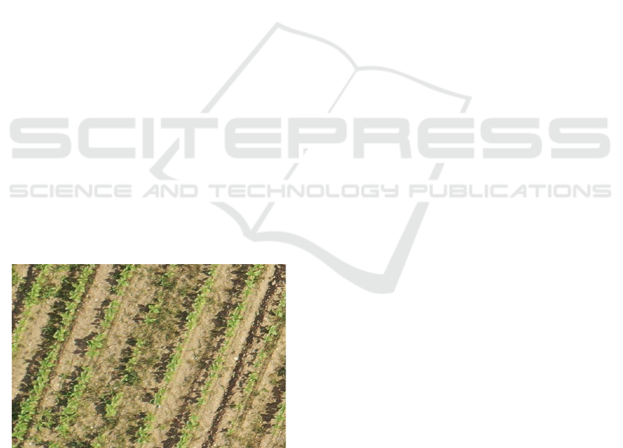
Figure 1 provides an example of an aerial image of

a sunﬂower ﬁeld. One can see rows of plants, here in a

rather late stage with overlap between plants, shadows

of various sizes and patches of weeds, especially on

the left side of the image.

Cependant, cette méthode ne permet pas de diﬀérencier les adventices des plants de tournesols car ce sont

deux objets de couleur verte. Nous avons donc cherché une autre méthode de segmentation de manière à éviter

que les adventices soient retenus (c’est à dire aﬃchés en blanc) à l’issue de cette étape.

2.1.2 Deuxième niveau par la méthode d’Otsu

On voit nettement sur les images que les tournesols apparaissent plus clairs que la plupart des adventices

(Figure 4). Nous avons alors exploité cette diﬀérence de teinte pour eﬀectuer une deuxième é tape d e segmen-

tation et essayer de s é p are r les pixels des tournesols des pixels des adventices.

Figure 4–ImagedelaparcelledeNiort.Aucentre,lesadventicesapparaissentplusfoncés.

Une méthode de segmentation automatique présentée par Otsu [12] permet de trouver automatiquement

une valeur de seuil optimale qui sépare deux groupes de pixels. Cette méthode est très employée pour l’analyse

d’images de champs et permet d’eﬀectuer une séparation automatique de pixels de deux teintes de vert diﬀérentes

(voir article [15] par exemple). Cette sép aration est réalisée grâce à un seuil qui se place au tomatiquement aﬁn

de former deux groupes de valeurs. Ces deux groupes sont trouvés de sorte que la variance intra-groupe soit

minimale, et la variance inter-groupe maximale (minimisation du rapport

intra

inter

). Nous avons appliqué cette

méthode de segmentation sur des images ExG (section 2.1.1)aﬁndeséparerlesvaleursd’indicesExGpropres

aux tournesols de celles propres aux adventices. L’algorithme de séparation d’Otsu ne diﬀérencie que deux

groupes. Or dans notre cas nous en avons 3 : le sol, les adventices et les tournesols. C’est pourquoi il faut

au préalable régler u n seuil minimal de départ de recherche qui exclut d’oﬃce le premier groupe de pixels

correspondant au sol, du reste. La séparation ne se fait alors qu’entre les pixels du groupe adventices et du

groupe tournesol. (Figure 5)

Figure 5–Agauche,l’imageoriginale.Au milieu l’image en indice ExG. Adroite,unproﬁlschématique

de l’histogramme des valeurs d’ExG sur lequel est appliqué l’algorithme de séparation d’Otsu. Encadré en

orange,lesvaleursd’ExGnontraitéesparl’algorithme(bornesupérieureﬁxéeparl’utilisateur).La ligne

verticale rouge correspond à une illustration d’un seuil de séparation possiblement trouvé par l’algorithme

d’Otsu

Cet algorithme permet de bien séparer les adventices des tournesols comme le montre la ﬁgure 6.En

revanche, la qualité de la séparation ad ventice-tournesol dépend de la valeur seuil de départ de recherche de

l’algorithme (ﬁxée par l’utilisateur).

Figure 1: Example of an aerial image from a sunﬂower ﬁeld.

The paper is structured as follows. Section 2 presents

the proposed approach. Information about the gen-

eration of synthetic datasets used in the experiments

is provided in Section 3 and the results of the experi-

ments are reported in Section 4. Section 5 concludes

and gives perspectives on future works.

2 THE METHOD

2.1 Analyzing the Spatial Relationships

Crop ﬁelds usually exhibit a geometrical design. The

rows of a crop ﬁeld are indeed usually parallel to

each other and evenly spaced. In addition, crops are

planted on the basis of a target density which induces

an even distance between two consecutive plants.

One main theme of this paper is to underline the

interest of researching and exploiting information on

the geometry of the objects in the images to be an-

alyzed. For crop ﬁelds images, in order to estimate

the inter-rows and inter-plants distances, the method

presented begins with (i) isolating the green areas of

the images; then (ii) rotating the images enough for

the rows to be collinear with the Y axis; and, ﬁnally,

(iii) applies a Fourier Transform (FT) analysis on the

signal produced by projecting the coordinates of the

green pixels on the X and Y axis.

2.1.1 Image Segmentation

Before estimating the inter-rows and inter-plants dis-

tances, it is necessary to identify the areas of the im-

ages corresponding to plants. To that end, we used

the vegetation index Excess Green (ExG) in associa-

tion with Otsu’s automatic segmenting method (Otsu,

1979; Guerrero et al., 2012; Guijarro et al., 2011;

erez-Ortiz et al., 2016). At the end of the segmen-

tation process, the RGB crop ﬁelds images are trans-

formed into black and white images, referred as Otsu

images, where the white pixels are expected to corre-

spond to a plant (crop or weed).

2.1.2 Vertically Adjusting the Images

To ease the estimation of the inter-rows and inter-

plants distances, the rotation of all the images of the

datasets was computed in order for the crop rows to

be oriented along the Y axis. This method succeeds

as long as two consecutive rows do not overlap with

each other or weed do not cover all the inter-rows

space. Should this happen, one can apply a ﬁlter to

the Otsu images in order to only keep the skeleton

of the crop rows in white. This can be implemented

with, for example, the midpoint encoding suggested

in (Han et al., 2004).

2.1.3 Estimating the Inter-rows and Inter-Plants

Distances

Items 1 and 3 on Fig. 2 illustrate how a periodic

signals is detected out of a vertically adjusted Otsu

Using Agents and Unsupervised Learning for Counting Objects in Images with Spatial Organization

689

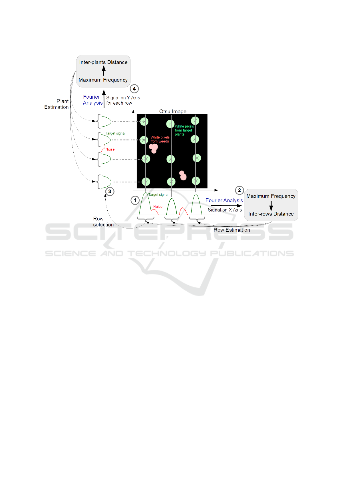
Figure 2: Fourier Analysis on the X and Y axis. The signal processed by the Fourier Transform is made from the projection

of the white pixels of the Otsu images on the X and Y axis.

image. Since the rows are assumed to have been re-

aligned with the Y axis, the periodicity of the posi-

tions of the rows appears on the X axis: the peaks

of the density distribution of the white pixels on the

X axis mirror the positions of the rows on the im-

age (item 1). The inter-rows distance is computed us-

ing a Fourier analysis on the density distribution and

keeping the maximal frequency thus found. The inter-

plants distance is then estimated using the projections

on the Y axis of the white pixels attributed to each row

(items 3 and 4).

2.2 A Multi-Agent Approach

Just like (Hofmann., 2019) in the case of remote im-

age sensing, we advocate the use of a multi-agent sys-

tem (MAS) which takes advantage of the knowledge

gathered on the geometry in the image. In the context

of the plant counting task, we identiﬁed four types of

agents that are organized hierarchically as shown in

Fig. 3. The agent at the top of the system is called

the Director Agent (DA), then come the Row Agents

(RAs), the Plant Agents (PAs) and ﬁnally the Pixel

Agents (PXAs). Each agent of one layer either acts on

its own or receive orders from an agent of the upper

layer: there is no communication between agents of

the same layer. The environments in which the agents

act are the vertically adjusted Otsu images.

2.2.1 The Director Agent

The DA can initialize or destroy RAs according to

the predictions made using the Fourier analysis (see

2.1.3) and decide when to stop the simulation. (see

2.1.3). It is also the one that computes the inter-plants

critical distance (IPCD) (see below).

Managing the Row Agents. At the beginning of

the simulation, the DA analyses the rows detected us-

ing the Fourier analysis in an attempt to exclude the

false positives: rows that are only made out of weeds.

A special procedure is devised to do so based on the

fact that these will be positioned in between real RAs

(rows consisting in plants).

Computing the Inter-Plants Critical Distance

(IPCD). Most of the decisions of the agents depend

ICAART 2021 - 13th International Conference on Agents and Artiﬁcial Intelligence

690

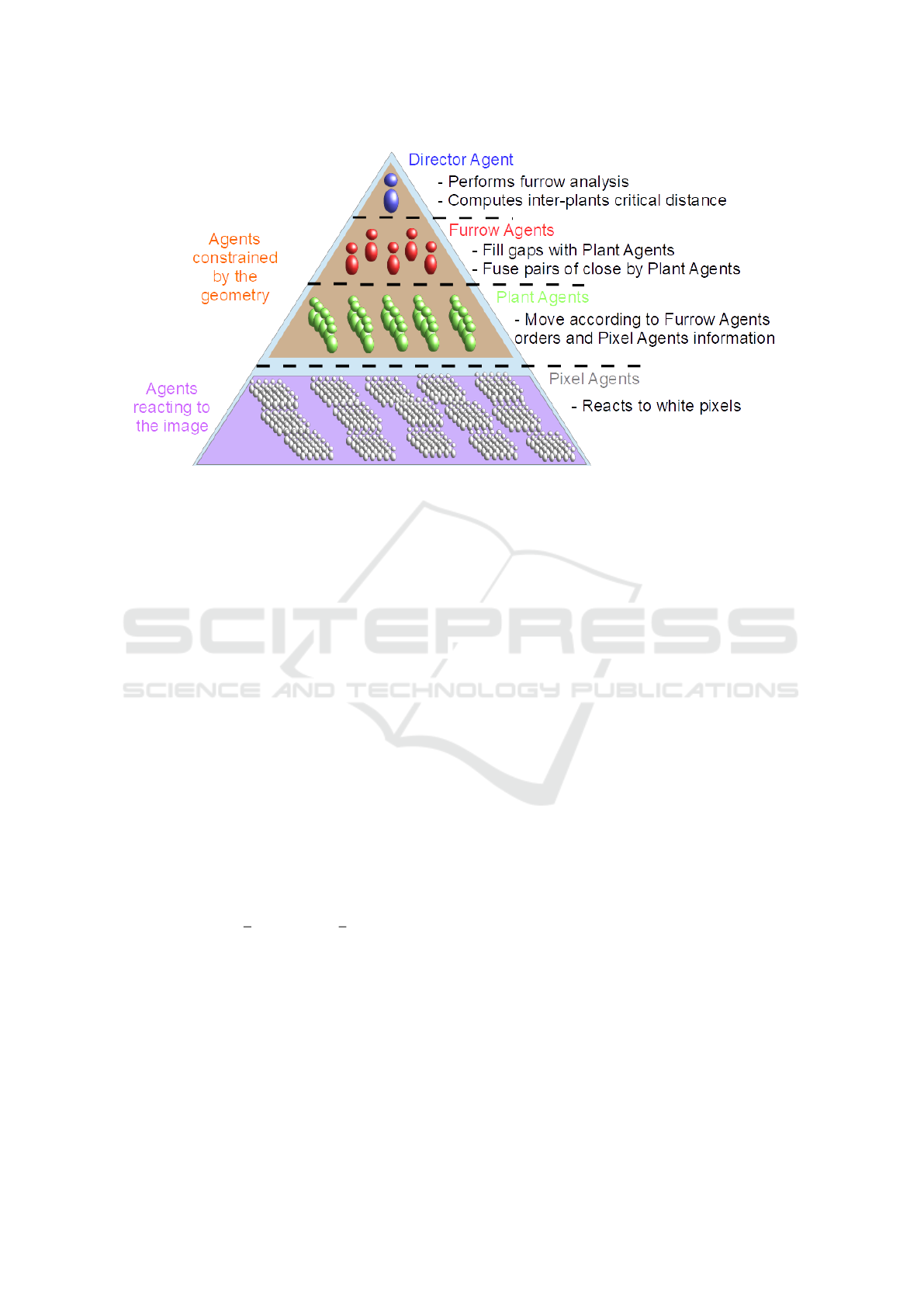
Figure 3: Hierarchical architecture of the multi-agent system.

on the IPCD. It is set equal to the maximum of the

density distribution of the inter-plant distances.

2.2.2 The Pixel Agents

The PXAs sense the Otsu images and are instantiated

by a PA. They become activated if they are positioned

on a white pixel and their position is determined by

the PA they are dependent upon.

2.2.3 The Plant Agents

The PAs are ultimately the most important agents for

the plant counting task. The number of PAs at the

end of the simulation determines the number of plants

detected in the frame of the image. Each PA has under

its supervision a group of PXAs that is centered on the

position of the PA. The role of the group of PXAs is to

guide the PA toward the most white parts of an Otsu

image (i.e. guiding them toward plants). Therefore, at

step i + 1 of the simulation, a PA moves on the mean

point of all its activated PXAs at step i:

(PA

i+1

,PA

i+1

) = (

∑

PXA∈A

PXA

∑

PXA∈A

PXA

)

(1)

with A the set of activated PXAs. The x and y are

the positions of the agents. Finally, a PA can decide

to decrease or increase its sensing area by eliminating

PXAs or by initializing new PXAs. In our simula-

tions, we set the goal of the PA to have between 20%

and 80% of its PXAs activated.

2.2.4 The Row Agents

RAs are instantiated by the DA according to the rows

detected by the Fourier Analysis (Fig. 2, item 2). In

turn, each RA ﬁrst initializes as many PAs as were

detected using the Fourier analysis (Fig. 2, item 4).

Because the Fourier analysis may miss plants at the

edges of the rows detected, additional PAs are evenly

spaced at 1.1ν times the IPCD, ν being the PAs fusing

factor (see next paragraph). At each simulation’s step,

RAs eliminate the PAs that are located in black areas

of the Otsu image: PAs with less than a proportion δ

of activated PXAs .

Filling and Fusing PAs. A RA may consider that

the distance between two consecutive PAs is either too

large or too small. It then decides to either ﬁll in the

gaps with new PAs of fuse the two involved PAs:

Decision =



Fill if |PA

i+1

− PA

| > µ IPCD

Fuse if |PA

i+1

− PA

| < ν IPCD

(2)

with µ and ν the ﬁlling and fusing factor respectively.

Constraining PAs Movements. In a crop ﬁeld, the

rows usually exhibit a linear shape, aligned with the Y

axis when adjusting the images (Section 2.1.2). The

plants that are part of the same row are thus expected

to be aligned. As a consequence, a RA can constrain

the moves of the PAs that it supervises in order to keep

them as aligned as possible.

Using Agents and Unsupervised Learning for Counting Objects in Images with Spatial Organization

691

2.2.5 Running the Simulation

The simulation consists in a sequence of actions that

the agents carry out in a deterministic order (Algo. 1).

The ﬁnal count of the plants occurs when the number

of PAs remains constant.

Algorithm 1: Simulation.

Input: max nb steps, µ, ν, δ, π

1 initialize DA, RAs, PAs, PXAs

/* Sec. 2.2.1 */

2 AnalyseRows(π)

3 ComputeIPCD()

4 AnalyseRowsEdges(ν, IPCD)

5 StopSimu ←− False

6 RE Eval ←− False

7 i ←− 1

8 while

i ≤ max nb steps & StopSimu = False do

/* Sec. 2.2.3 */

9 MoveToMeanPoint()

/* Sec. 2.2.4 */

10 ConstrainPAsXMovement()

11 FillOrFusePAs(µ, ν, IPCD)

/* Sec. 2.2.3 */

12 AdaptSize()

/* Sec. 2.2.4 */

13 DestroyLowActivityPAs(δ)

14 if Nb PAs

− Nb PAs

i−1

= 0 then

15 if RE Eval = False then

16 DA ComputeIPCD()

17 RE Eval ←− True

18 else

19 StopSimu ←− True

20 end

21 else

22 RE Eval ←− False

23 end

24 i←− i+1

25 end

3 SYNTHETIC DATASETS

Training an automatic counting algorithms requires

large data sets with at the very least hundreds of im-

ages, with thousands of objects, each of them to be

labeled. In the case of plant counting, there are no

publicly available data sets. This entails a lack of la-

beled training data and a problem of reproducibility

Figure 4: Parameters involved in the placement of crops

along rows. The red labels are parameters undergoing ran-

domization.

of experiments.

The solution we adopted is to use a virtual envi-

ronment engine to generate artiﬁcial crop ﬁelds. They

are indeed nowadays able to generate very realistic

images, and the labelling of the objects is automatic.

We chose to use the game engine Unity (Technolo-

gies, 2020).

3.1 The Field Generator

The parameters mainly manage the surface of the

ﬁeld, the virtual crop, the weed, the sun and the sim-

ulated drone. Figure 5 describes the UAV ﬂight plan.

Crops position in the ﬁeld are based on several pa-

rameters shown in red on Figure 4. All parameters

except the growth probability are drawn randomly.

Weeds cannot be expected to follow any geometry at

the scale of the ﬁeld but they can regularly be found

clustered together. This is why we used the Perlin

Noise (Perlin, 1985) to generate spaces on the crop

ﬁeld where the weeds would be present.

3.2 Content of the Datasets

Plants may overlap as the plants grow. It is assumed

that the overlap interferes with the signal used by the

counting method, and previous studies on automatic

counting of plants from UAV images have raised that

the difﬁculty of the task increases with the proportion

of crop overlap (Garc

ıa-Mart

ınez et al., 2020). In or-

der to assess this effect, we generated three datasets

with three different levels of overlap between crops.

The plants are separated (S) from each other in the

ﬁrst dataset; they overlap for some leaves and do not

overlap for others (B) in the second datase; and ﬁ-

nally, the third dataset exhibits overlap (O) between

neighbouring plants. The dataset (S) is considered

ICAART 2021 - 13th International Conference on Agents and Artiﬁcial Intelligence

692

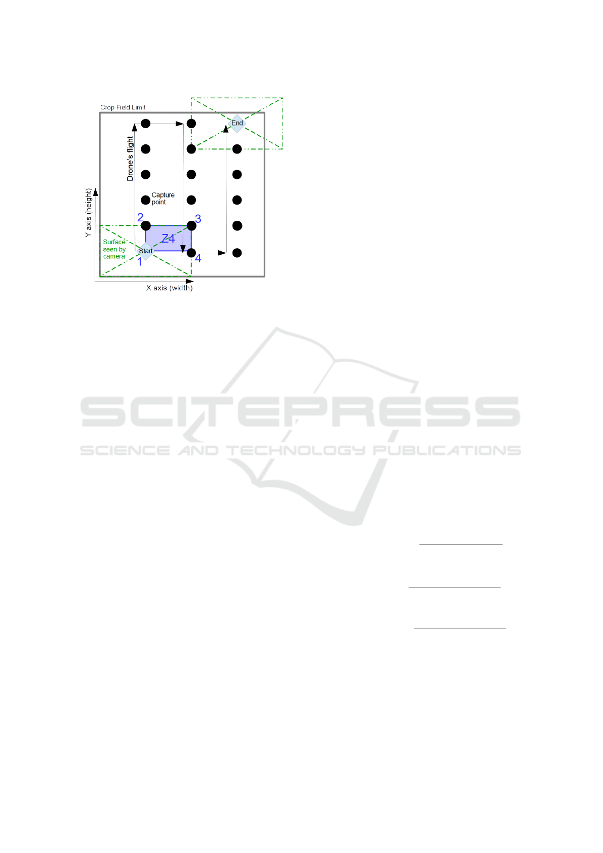
Figure 5: Scheme of a UAV ﬂight plan above the virtual

crop ﬁeld. The start position is calibrated to capture the

bottom left corner of the ﬁeld. The other capture points

are calculated depending on the image overlap conﬁgured

on the X and Y axis (here, 50% on both). As a result, the

images of the upper and right limit of the ﬁeld may go over

these. The area named Z4 is subsequently captured four

times, one by each of the four captured points numbered in

blue.

easy, (B) is intermediate and (O) is difﬁcult. Aside

from varying the scale of the plant 3D model to sim-

ulate its growth, the parameters used to generate the

ﬁelds are similar for all three datasets. Each crop ﬁeld

was generated with an inter-rows distance of 70 cm

and an inter-plants distance of 20 cm with 5% vari-

ability. This yields a target average of 7 plants/m

which matches typical sunﬂower crop ﬁelds. The

plant growth probability was set to 0.8. The Perlin

noise threshold used to generate the surfaces where

weed grows was set to 0.75 while the weed growth

probability was set to 0.6. In each of these datasets,

100 crop ﬁelds were generated, and from each of them

four images were taken. So, each dataset contains

400 images which amounts to 1200 images in total.

To take pictures of the virtual ﬁelds, we simulated a

short drone ﬂight plan that covers the lower left cor-

ner of the ﬁeld as it moves once along the height and

width of the ﬁeld (see the blue numbers on Fig. 5).

We have conﬁgured the motion of the simulated drone

to overlap the image by 50% along both their height

and width, as is usual with images from UAVs.

Fig. 6 gives an example of an image of a virtual

crop ﬁeld. Fig. 6b is the same image after an Otsu

ﬁlter has been applied and the image has been reori-

ented so that the rows are aligned with the Y axis. (see

sections 2.1.1 and 2.1.2).

4 EXPERIMENTS AND RESULTS

The method we propose is a two steps method with

the ﬁrst phase that detects and estimates the spatial

structure, and the second phase which, starting from

this structure identiﬁes the objects.

The goal of the experiments carried out is three-

fold. First, to assess the performance of the ﬁrst

phase alone in counting plants, second, to measure

the added value of the second phase based on a multi-

agent approach, and, third, to look at the gain of per-

formance, if any, when parts of a ﬁeld are covered

by multiple passes of the UAV and a redundancy of

information follows (see area Z4 in Figure 5 for an

example).

First, we present the rules under which we consid-

ered that the method had successfully detected a plant

and how the counting performance was measured.

4.1 Assessing the Results

In order to measure the performance of the Fourier

analysis alone, the rule is that if the plant position,

which is known in synthetic data sets, falls within a

40 square pixel area of a predicted position, then this

is counted as a true positive (TP).

For the MAS, we considered that a PA detected a

plant if that plant was located within the sensing area

deﬁned by the PXAs of the PA. If two PA happen to

detect the same plant, then only one PA is counted as

TP and the other is counted as a false positive (FP).

Additionally, a PA or a prediction from the Fourier

analysis that does not contain a plant in their sensing

area are also considered as FP. Finally, a plant that has

not been detected is counted as a false negative (FN).

In addition to these three indicators, three scores are

computed:

Detection Accuracy =

T P

Total number of PAs

(3)

Detection Recall =

T P

Total number of Plants

(4)

Counting Accuracy =

Total number of PAs

Total number of Plants

(5)

These scores are later referenced as DAc, DR and CA

respectively.

In the following, we compare the performances of

the Fourier analysis alone (Section 4.2), of the multi-

agent approach from a single image of the area (Sec-

tion 4.3), and of a technique that takes into account

that several images (up to four) can cover a given area

(Section 4.4).

Using Agents and Unsupervised Learning for Counting Objects in Images with Spatial Organization

693

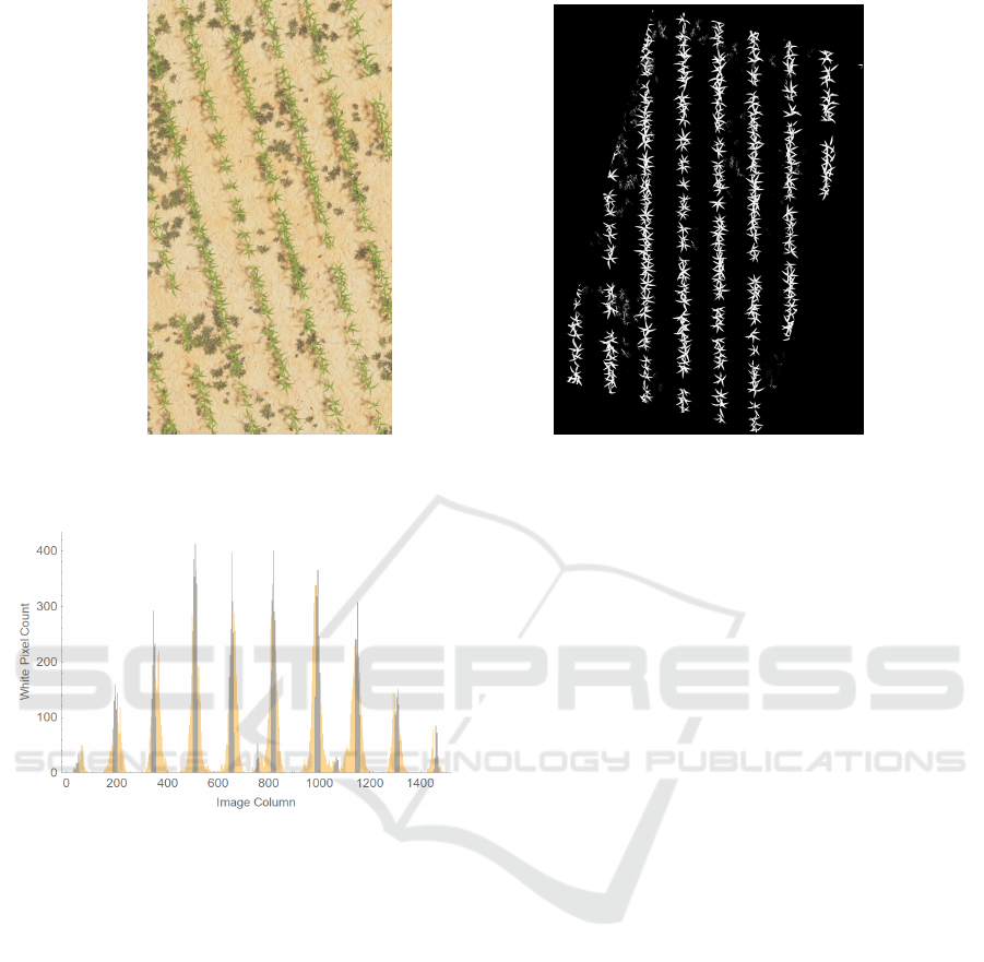
(a) An image of a virtual ﬁeld (b) Otsu image vertically adjusted

Figure 6: Example of a an synthetic image and its vertically adjusted Otsu image.

Figure 7: Example of row detection thanks to Fourier anal-

ysis. The histogram in yellow results from the projection of

the white pixels of an Otsu Image on the X axis. The blue

parts of the histogram are the detected rows.

4.2 Detecting the Spatial Structure and

Counting

As explained in Section 2.1.3, we use Fourier analysis

to approximate the spatial structure in an image. We

ﬁrst try to discover the rows and then to locate plants

within the presumed rows. This relies on the analy-

sis of the density distribution of the projection of the

white pixels from an Otsu image on the X or Y axis

(Fig. 7 shows such a density distribution (in yellow)

as well as the detected peaks (in blue)). Notice that

the largest peaks indeed correspond to rows, but that

weeds can also produce peaks, albeit smaller ones.

The results obtained for the three scores are sum-

marized in Table 1 in the line Fourier while Fig. 8

provides details on the distribution of the counting ac-

curacies (CAs) (violet boxes indicate the results of the

Fourier analysis).

It is apparent that the Fourier analysis alone tends

to underestimate the number of plants on dataset (S),

(the well separated plants) (12% on average) while

over estimating this number on datasets (B) (between

separated and overlapping) (by 3%) and (O) (overlap-

ping plants) (by 7% on average). Why is it so?

For dataset (S), the plants are well separated, but

this also entails that the peaks of the histogram used

by the Fourier analysis are rather narrow, and one con-

sequence is that if a peak is slightly off a predicted

position by the analysis, it may be entirely missed by

it. This may result in ignoring existing rows or plants

within a row.

For datasets (B) and (O), the overlapping leaves

between plants induces noise that leads the Fourier

analysis dedicated to the plants identiﬁcation to ﬁnd a

slightly higher frequency than the actual target. This

results in overestimating the number of plants. Over-

all, still, taking into account that the Fourier analysis

is in fact used only to estimate the spatial relationships

between plants on crop ﬁelds, the counting results are

surprisingly good.

4.3 Effect of the Multi-Agents Analysis

The multi-agent stage initializes the PAs using the

predictions made by the detector of spatial relation-

ships, and then let the PAs evolve and converge to-

wards presumed plants. The question is: how much

this can improve the counting performance? In which

way can it correct false positives and false negatives?

In our experiments on plant counting, we ran

ICAART 2021 - 13th International Conference on Agents and Artiﬁcial Intelligence

694

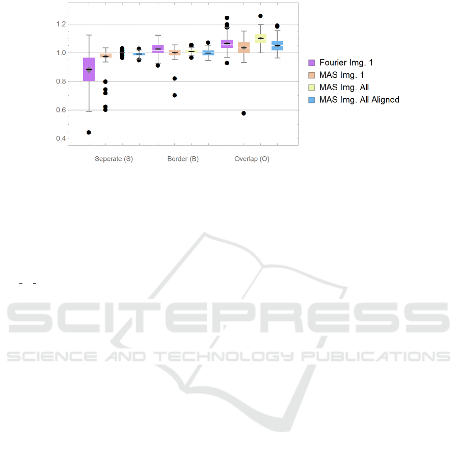
Figure 8: Results on Counting Accuracy (CA). The colors of the whisker boxes indicate the method used to count the number

of plants. With Fourier Img. 1 we counted the plants with the Fourier analysis on one imagefor each of the 100 ﬁelds of

the dataset. The same images were used with MAS Img. 1 that counts the plants using the MAS. MAS Img. All and MAS

Img. All Aligned are methods that exploit the redundancy when several images cover the same area in a ﬁeld. The black dots

represent outliers. The boxes’ lower and upper limits indicate the 0.25-th and 0.75-th percentile respectively. The median is

represented on each box by a white line mark while the mean is represented as a black line mark. The grey diamond represents

the interval of conﬁdence. Non-overlapping diamond between pairs of boxes are equivalent to rejecting the null hypothesis of

equal means of a two-sample t-Test.

the simulations with the following parameters values:

max nb steps = 50, µ = 1.5, ν = 0.5, δ = 0.01 and

π = 0.0001. max nb steps was set as an upper limit of

the number of steps of the simulation which has never

been reached in our experiments. The values µ and

ν were chosen for geometric reasons. ν is the PAs’

fusion factor; a value of 0.5 means that two PAs per-

fectly positioned on consecutive plants will absorb a

wrongly positioned PA in-between them which is de-

sirable. µ is the PAs’ ﬁlling factor; if two PAs are per-

fectly positioned on plants but another plant has been

missed in-between them, then a value of 2 should al-

low its detection. However a value of 1.5 proved to

be better during tests. Lowering the values of δ and

π will lead the simulation to overestimate the number

of plants while raising them will lead to underesti-

mation. These values were optimized by repeatedly

testing the system on training synthetic datasets. The

reported results have been obtained on test datasets,

different from the training ones.

As can be seen in Fig. 8 and in Table 1, the re-

sults show that the multi-agent phase signiﬁcantly im-

proves the counting performance. For the (S) and (B)

datasets, the mean value is closer to the value 1 (ap-

proximately 0.98 instead of 0.87 for the Fourrier anal-

ysis alone), which means that the estimated number

of plants is close to the correct one, and the conﬁ-

dence interval is much narrowed (standard deviation

of 0.04 instead of 0.11). The gain is less pronounced

on the (O) dataset. Even if the distribution of the re-

sults are very similar between the Fourier analysis and

the multi-agent one (violet and orange boxes on Fig.

8), the average for the multi-agent analysis is signif-

icantly lower than the average of the Fourier analy-

sis as indicated by the fact that the grey diamonds on

the boxes do not overlap (non-overlapping diamonds

mean that the null hypothesis of equal means can be

rejected using a 2-sample t-Test).

It is thus apparent that the proposed two step

method: ﬁrst detecting a structure, then using a MAS

to reﬁne the counting, gives very promising results.

But, most of the areas of a crop ﬁeld are covered by

several different images from UAVs (up to four times

in the example of Figure 5). Is it possible then that

even these good results can be improved by resorting

to the redundancy thus offered?

4.4 Exploiting Image Overlapping

A common practice when acquiring images of crop

ﬁelds is to let consecutive images overlap each other.

One of the main motivation for this is to avoid that

plants located at the edges of an image are only par-

tially visible, and thus ignored. Another motivation is

the hope that the mistakes made on an image can be

compensated on another image that partially covers

the same area. In our case, the synthetic datasets were

built with 50% overlap on the height and width of the

images. As an illustration, in our example, it exists

an area (e.g. Z4) that is covered by all four images.

The results when combining the informations coming

from the four images are presented under the name

MAS Img. All in Table 1 and Fig. 8. Another vari-

ant of this algorithm (called MAS Img. All Aligned)

Using Agents and Unsupervised Learning for Counting Objects in Images with Spatial Organization

695

Table 1: Average scores results on the three datasets. Standard deviation is in parenthesis. Values were rounded to the second

digit.

Datasets Separate (S) Border (B) Overlap (O)

Scores DAc DR CA DAc DR CA DAc DR CA

Fourier

Img. 1

0.93

(0.04)

0.82

(0.11)

0.88

(0.12)

0.87

(0.06)

0.89

(0.05)

1.03

(0.04)

0.81

(0.05)

0.86

(0.05)

1.07

(0.05)

MAS Img.

0.99

(0.01)

0.97

(0.07)

0.97

(0.07)

0.98

(0.02)

0.98

(0.04)

1.00

(0.04)

0.83

(0.05)

0.86

(0.06)

1.03

(0.07)

MAS Img.

All

0.99

(0.01)

0.99

(0.01)

1.00

(0.01)

0.99

(0.02)

1.00

(0.01)

1.01

(0.02)

0.88

(0.04)

0.96

(0.02)

1.10

(0.05)

MAS Img.

All Aligned

0.99

(0.01)

0.98

(0.01)

0.99

(0.02)

0.99

(0.02)

0.98

(0.02)

1.00

(0.02)

0.90

(0.04)

0.94

(0.03)

1.05

(0.05)

was introduced with the motivation that aligning the

N images covering a given area could help the clus-

tering procedure to gather relevant PAs.

The results reported in Table 1 and in Figure 8

show that combining information from the analysis

of several images brings improvement in the count-

ing accuracy for the (S) and (B) datasets. For the (O)

dataset, the variant MAS Img. All Aligned is to be pre-

ferred to the MAS Img. All method, while MAS Img.

All is better than MAS Img. All Aligned on the (S)

and (B) datasets. If the counting accuracy of the com-

bined method is slightly lower than for the method

analyzing only one image for the (O) datasets (1.05

instead of 1.03), on the other hand the detection accu-

racy (DA) is signiﬁcantly improved from 0.83 to 0.90

which means that the plants are better recognized.

Overall, combining information from several im-

ages seems to be a good strategy.

4.5 Application to Real Images

We also applied the method to a subset of the dataset

of real crop ﬁelds provided by Christophe Sausse

from Terres Inovia.

In total, the dataset contains 2111 non-labelled

images from which we randomly extracted 50 that

were manually labeled and used to test our method.

The images mix areas where the plants are well sepa-

rated and areas where the leaves of one plant overlap

with those of its neighbors in the same row. In ad-

dition, the drone captured the original images at an

altitude of 30m (compared to 10m for the synthetic

data) and the sunﬂowers overlap with many weeds in

some images, making it sometimes difﬁcult, even for

a human, to visually identify the sunﬂowers. It is thus

fair to say that the chosen subset of data contains im-

ages comparable to the ones of the (S), (B) and (O)

synthetic datasets.

Our method yielded an average counting accuracy

of 1.03 for a standard deviation of 0.12 on the 50 im-

ages subset. The detection accuracy and detection re-

call fared at 0.87 and 0.90 respectively for a standard

deviation of 0.14 for both. These scores are at least as

good as the ones reported in the state of the art (see

Section 4.6). Furthermore, they are quite close to the

results obtained on the synthetic dataset even if the

standard deviation is larger.

This conﬁrms that using synthetic datasets for tun-

ing the method we propose is a promising procedure,

effectively leading to good results on real data.

4.6 The State of the Art

Counting objects can be done through the detection of

the objects, or it can be done from a density estimate,

usually directly from an analysis at the pixel level of

the image. In the ﬁrst case, object detection relies

either on some prior knowledge of the shape of the

objects to be counted or on machine learning to rec-

ognize objects. Deciding which templates are useful

is generally difﬁcult, while using supervised learning

requires (very) many labeled images and large com-

puting resources, for example using deep neural net-

works. On the other hand, density estimation seems

simpler but it still requires large training sets and

yields coarser estimates of the number of objects in

an image. Both approaches, object-based and density-

based, are subject to large errors when objects are oc-

cluded or overlapping.

For plant counting, (Garc

ıa-Mart

ınez et al., 2020)

is an example of the template approach. In their maize

plant counting experiments, they selected 4 to 12 tem-

plates and used a Normalized Cross-Correlation tech-

nique to estimate the number of plants. The method

requires that representative plants in the images be

chosen, and no recipe is given for this. They obtain a

percentage or error of 2.2% when using 12 templates,

but acknowledge that the performance drops to 25.7%

when the plants overlap.

In their paper, (Ribera et al., 2017) use deep neural

ICAART 2021 - 13th International Conference on Agents and Artiﬁcial Intelligence

696

networks to learn how to recognize sorghum plants.

They describe the rather involved preprocessing and

formatting steps that are necessary before learning

can take place. They also had to develop a technique

to increase the number of labelled training images.

Learning itself took between 50,000 and 500,000 it-

erations which entails a very heavy computing load.

They obtained a Mean Absolute Percentage Error of

6,7%. It is not possible to know if the data sets used

included overlapping plants or not.

The density-based approach is illustrated in

(Gn

adinger and Schmidhalter, 2017). They ﬁrst elim-

inate what can be presumed to be weeds and para-

sitic signals using a clustering method. Then they set

thresholds on different wavelengths in order to clas-

sify pixels as belonging to plants or not. This requires

some ﬁne tuning. They obtain error rates around 5%

with fairly large standard deviations. Here too, plant

overlapping leads to a deterioration in performance.

5 CONCLUSIONS

With the generalization of devices for taking images,

it is increasingly critical to develop reliable and trans-

parent image vision systems (Olszewska, 2019). This

paper has introduced a new method to count objects

while satisfying these constraints. It is applicable

when objects are spatially organized according to a

regular pattern. The method ﬁrst detects the pattern

and then uses it to seed agents in a MAS. The method

is simple, requiring no complex ﬁne tuning of param-

eters, the tricky deﬁnition of templates or costly learn-

ing. In fact, it requires very modest computing re-

sources. In a series of extensive experiments on con-

trolled data sets and real aerial images of crop ﬁelds,

the method yielded state of the art or better perfor-

mance when the objects are well-separated and ex-

ceeded the best known performances when the objects

overlap. For future work, we plan to test the method

on other other object counting problems with differ-

ent geometries such as counting people in stadiums

or performance halls or vehicles in parking lots.

ACKNOWLEDGEMENTS

We thank Terres Inovia for sharing their dataset of

crop ﬁelds images captured with a UAV.

REFERENCES

Garc

ıa-Mart

ınez, H., Flores-Magdaleno, H., Khalil-

Gardezi, A., Ascencio-Hern

andez, R., Tijerina-

avez, L., V

azquez-Pe

na, M. A., and Mancilla-Villa,

O. R. (2020). Digital count of corn plants using im-

ages taken by unmanned aerial vehicles and cross cor-

relation of templates. Agronomy, 10(4):469.

adinger, F. and Schmidhalter, U. (2017). Digital counts

of maize plants by unmanned aerial vehicles (uavs).

Remote sensing, 9(6):544.

Guerrero, J. M., Pajares, G., Montalvo, M., Romeo, J., and

Guijarro, M. (2012). Support vector machines for

crop/weeds identiﬁcation in maize ﬁelds. Expert Sys-

tems with Applications, 39(12):11149–11155.

Guijarro, M., Pajares, G., Riomoros, I., Herrera, P., Burgos-

Artizzu, X., and Ribeiro, A. (2011). Automatic seg-

mentation of relevant textures in agricultural images.

Computers and Electronics in Agriculture, 75(1):75–

83.

Han, S., Zhang, Q., Ni, B., and Reid, J. (2004). A guid-

ance directrix approach to vision-based vehicle guid-

ance systems. Computers and Electronics in Agricul-

ture, 43(3):179–195.

Hofmann., P. (2019). Multi-agent systems in remote sens-

ing image analysis. In Proceedings of the 11th In-

ternational Conference on Agents and Artiﬁcial Intel-

ligence - Volume 1: ICAART 2019, pages 178–185.

INSTICC, SciTePress.

Olszewska, J. (2019). Designing transparent and au-

tonomous intelligent vision systems. In Proceed-

ings of the 11th International Conference on Agents

and Artiﬁcial Intelligence - Volume 2: ICAART 2019,

pages 850–856. INSTICC, SciTePress.

Otsu, N. (1979). A Threshold Selection Method from

Gray-Level Histograms. IEEE Transactions on Sys-

tems, Man, and Cybernetics, 9(1):62–66. Conference

Name: IEEE Transactions on Systems, Man, and Cy-

bernetics.

erez-Ortiz, M., Pe

na, J. M., Guti

errez, P. A., Torres-

anchez, J., Herv

as-Mart

ınez, C., and L

opez-

Granados, F. (2016). Selecting patterns and features

for between-and within-crop-row weed mapping us-

ing uav-imagery. Expert Systems with Applications,

47:85–94.

Perlin, K. (1985). An image synthesizer. ACM SIG-

GRAPH Computer Graphics, 19(3):287–296.

Ribera, J., Chen, Y., Boomsma, C., and Delp, E. J. (2017).

Counting plants using deep learning. In 2017 IEEE

global conference on signal and information process-

ing (GlobalSIP), pages 1344–1348. IEEE.

Technologies, U. (2020). Unity 2019.4.1.

Zou, Z., Shi, Z., Guo, Y., and Ye, J. (2019). Object Detec-

tion in 20 Years: A Survey. arXiv:1905.05055 [cs].

arXiv: 1905.05055.

Using Agents and Unsupervised Learning for Counting Objects in Images with Spatial Organization

697