
LigityScore: Convolutional Neural Network for Binding-affinity
Predictions
Joseph Azzopardi
1 a
and Jean Paul Ebejer
1,2 b
1
Department of Artificial Intelligence, University of Malta, Msida, MSD 2080, Malta
2
Centre for Molecular Medicine and Biobanking, University of Malta, Msida, MSD 2080, Malta
Keywords:
Virtual Screening, Structure-based Virtual Screening, Scoring Function, Pharmacophoric Interaction Point,
Machine Learning, Deep-Learning, Convolutional Neural Networks, LigityScore.
Abstract:
Scoring functions are at the heart of structure-based drug design and are used to estimate the binding of ligands
to a target. Seeking a scoring function that can accurately predict the binding affinity is key for successful
virtual screening methods. Deep learning approaches have recently seen a rise in popularity as a means to
improve the scoring function having as a key advantage the automatic extraction of features and the creation
of a complex representation without feature engineering and expert knowledge. In this study we present
LigityScore1D and LigityScore3D, which are rotationally invariant scoring functions based on convolutional
neural networks. LigityScore descriptors are extracted directly from the structural and interacting properties
of the protein-ligand complex which are input to a CNN for automatic feature extraction and binding affinity
prediction. This representation uses the spatial distribution of Pharmacophoric Interaction Points, derived from
interaction features from the protein-ligand complex based on pharmacophoric features conformant to specific
family types and distance thresholds. The data representation component and the CNN architecture together,
constitute the LigityScore scoring function. The main contribution for this study is to present a novel protein-
ligand representation for use as a CNN based SF for binding affinity prediction. LigityScore models are
evaluated for scoring power on the latest two CASF benchmarks. The Pearson Correlation Coefficient, and
the standard deviation in linear regression were used to compare and rank LigityScore with the benchmark
model, and also to other models recently published in literature. LigityScore3D has achieved better overall
results and showed similar performance in both CASF benchmarks. LigityScore3D ranked 5
th
place for the
CASF-2013 benchmark , and 8
th
for CASF-2016, with an average R-score performance of 0.713 and 0.725
respectively. LigityScore1D ranked 8
th
place for the CASF-2013 and 7
th
place for CASF-2016 with an R-
score performance of 0.635 and 0.741 respectively. Our methods show relatively good performance when
compared to the Pafnucy model (one of the best performing CNN based scoring functions), on the CASF-
2013 benchmark using a less computationally complex model that can be trained 16 times faster.
1 INTRODUCTION
Structure-based virtual screening (SBVS) employs
the known 3D protein structure to apply computa-
tional methods that measure the ability of a small
molecule to bind to the target protein. Docking is
one of the most popular SBVS methods and is used
to validate the ability of small molecules to bind to
the target structure in a typical ’lock and key’ fash-
ion (Ching et al., 2018). During the docking process
many possible ligand conformers, or docking poses,
are iteratively tested at the binding site to find a suit-
a
https://orcid.org/0000-0001-9058-5361
b
https://orcid.org/0000-0003-0888-2637
able ligand pose yielding the best binding affinity.
The binding affinity of a particular pose is determined
by the scoring function (SF) of the docking program.
The SF is therefore crucial for docking programs in
SBVS and can be defined as ”Estimating how strongly
the docked pose of a ligand binds to the target” (Ain
et al., 2015). Scoring functions are typically used
for fast evaluation of protein-ligand interactions, so
building an efficient and powerful SF is a means of
accelerating the virtual screening (VS) process. The
SF is considered the foundation in SBVS and used in
the following areas for hit discovery and optimization
(Ragoza et al., 2017):
1. Pose Prediction: Predict the shape of the ligand
38
Azzopardi, J. and Ebejer, J.
LigityScore: Convolutional Neural Network for Binding-affinity Predictions.
DOI: 10.5220/0010228300380049
In Proceedings of the 14th International Joint Conference on Biomedical Engineering Systems and Technologies (BIOSTEC 2021) - Volume 3: BIOINFORMATICS, pages 38-49
ISBN: 978-989-758-490-9
Copyright
c
2021 by SCITEPRESS – Science and Technology Publications, Lda. All rights reserved

which gives the best binding affinity.
2. Ranking: Ranking of molecules with known
binding pose in order of the binding affinity for
a given protein target.
3. Classification: Given the binding-pose, classify
whether a small molecule is active or inactive for
a given 3D structure of a target protein.
Intense research has been carried out over the
years on this problem, however improving the accu-
racy for binding affinity prediction has proven to be
a non-trivial task (Ain et al., 2015). Despite sev-
eral advances in binding affinity prediction, the cur-
rent binding affinity estimates are still not accurate
enough leading to high false positive rates (Zheng
et al., 2019). The work described in this paper fo-
cuses directly on the SF layer of SBVS and tack-
les this problem by finding an alternative data repre-
sentation of the protein-ligand complex and then ap-
plies a Convolutional Neural Network (CNN) regres-
sion model to implement the SF. Deep Learning (DL)
models have achieved remarkable success in various
areas such as computer vision (Szegedy et al., 2015)
and natural language processing (Goldberg, 2016).
Inspired by this success, the use of DL and in particu-
lar CNNs have naturally become an obvious strategy
to apply for computer aided drug design. Conven-
tional ML techniques, such as Random Forests and
Support Vector Machines, are limited to process raw
data, requiring careful feature engineering and expert
domain knowledge (LeCun et al., 2015). Deep learn-
ing methods aims to reduce feature engineering and
automatically extract the salient feature information
from the input data using multiple hidden layers, pro-
vided it has a suitable representation of the molecu-
lar interactions between the protein and ligand (P
´
erez-
Sianes et al., 2019). Therefore, our strategy is to allow
deep learning models to learn the underlying molec-
ular interactions so that this learned information can
be reapplied to other protein targets for exploration
of novel ligands, without the need to incorporate ex-
pert chemical knowledge. Our work is evaluated us-
ing the CASF-2013 (Li et al., 2014) and CASF-2016
(Su et al., 2018) benchmarks and is also compared
to other recently-published SF methods that use the
same benchmarks.
The first deep neural network (DNN) used for VS
was introduced by the winners of the 2012 Kaggle
Merck Molecular activity challenge (Kaggle, 2012)
where the team applied a multi-task deep feed for-
ward network for quantitative structure-activity. This
work was later published by Ma et al. (2015) and gen-
erated a lot of interest and excitement around the use
of DL in this field. Ma et al. (2015) have achieved an
average Pearson correlation coefficient of 0.496 us-
ing a multi-task DNN compared to the 0.423 obtained
when using a Random Forest model.
The Convolutional Neural Network (CNN) is one
of the most common DL architectures used for SFs
(Rifaioglu et al., 2018; P
´
erez-Sianes et al., 2019). The
CNN uses a number of sequential layers of convolu-
tions and pooling modules to encode the hidden fea-
tures of the data, and then use a fully connected feed-
forward neural network for classification or regres-
sion. One of the advantages of CNNs in the area of
structure-based drug design is its ability to capture lo-
cal spatial information interactions between protein-
ligand complexes. In recent years, many CNN models
have been applied to SF development (Ragoza et al.,
2017; Stepniewska-Dziubinska et al., 2017; Jim
´
enez
et al., 2018; Zheng et al., 2019; Liu et al., 2019).
Ragoza et al. (2017) were the first to use CNNs
to implement a DL scoring function that predicts
the docking score for a drug target interaction which
was then used for SBVS and pose prediction. How-
ever, Sieg et al. (2019) later showed that their model
was effected by non-causal bias. One of the most
promising DL SF models, Pafnucy, was proposed by
Stepniewska-Dziubinska et al. (2017) where the au-
thors achieved a Pearson Coefficient, R, for the pre-
dicted versus experimental binding affinity of 0.70 on
the CASF-2013, and 0.78 on the CASF-2016 bench-
marks respectively. Pafnucy uses a 3D CNN model
with a 4D tensor to represent 19 protein-ligand fea-
tures in 3D. The 4D tensor includes discretised atom
location in the first three dimensions, whilst the fea-
tures for the particular atom are encoded in the fourth
dimension.
Jim
´
enez et al. (2018) also utilise a 3D CNN model
termed K
deep
and achieved state of the art results on
the CASF-2016 test with an R value of 0.82. Their
input features use a 3D voxel representation where
each channel encodes a particular property of the
atom. Each protein-ligand complex is represented by
a 4D tensor, where each 3D hyperplane represents the
protein-ligand complex with respect to a particular
property only. The eight properties chosen for K
deep
include: hydrophobic, aromatic, hydrogen bond ac-
ceptor (HBA), hydrogen bond donor (HBD), cation,
anion, metallic, and excluded volume. A recent study
proposed by Zheng et al. (2019) compares their model
to Stepniewska-Dziubinska et al. (2017) and criticize
the Pafnucy model that the protein-ligand interactions
in a 3D grid box of 20
˚
A are not sufficient to capture
all the protein-ligand interactions, and suggest that
other long-range interactions outside the 20
˚
A , termed
non-local electrostatic interactions are also important.
To capture all the interactions between protein-ligand
LigityScore: Convolutional Neural Network for Binding-affinity Predictions
39
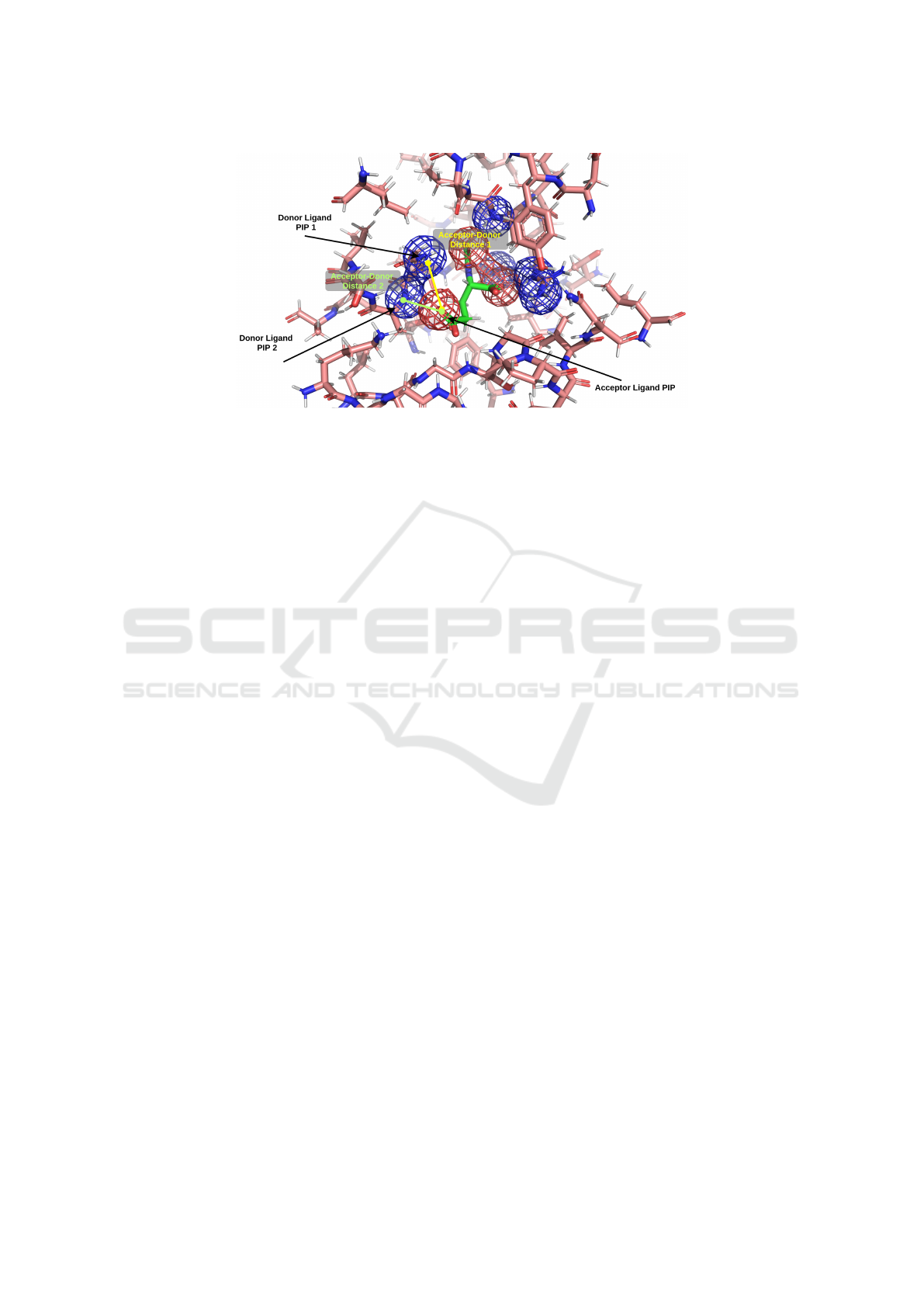
Figure 1: PIP pair interaction between two hydrogen bond donor protein PIPs (blue mesh), and a hydrogen bond acceptor
ligand PIP (red mesh). Other PIPs not shown for clarity. For each PIP interaction the distance between the geometric centres
of the PIPs is calculated.
complexes, Zheng et al. (2019) divide all the 3D space
of the binding site into a number of shells or zones and
count the number of different element-to-element in-
teractions within each shell. Their experiments show
that the shells closer to the ligand are more impor-
tant, as was intuitively expected, however they also
show that non-local interactions have significant im-
portance. Zheng et al. (2019) compare their method
OnionNet to another recent model, AGL-Score by
Nguyen and Wei (2019a). Both methods use CASF
as an evaluation benchmark. Zheng et al. comment
that OnionNet provides a more complete local envi-
ronment and improves the affinity prediction perfor-
mance with an R of 0.833. To date this represents the
best performing ML scoring function. The better re-
sults are achieved by adding novel features relating to
the physical and biological information of the com-
plex using graph theory.
One of the limitations of Pafnucy and K
deep
is the
dependency on the coordinate frame. The represen-
tation can be thought of as one snapshot of the struc-
ture. However, if the orientation from where the snap-
shot is changed, a different representation of the same
protein-ligand complex is obtained. The authors have
worked around this limitation by introducing different
systematic rotations of the same input during train-
ing. However, these might present additional chal-
lenges when testing novel complexes that can take
different orientations. This limitation has led us to
explore methods that are inherently rotationally in-
variant. One such model that is not dependent on
the coordinate frame is Ligity developed by Ebejer et
al. (2019). Ligity is a hybrid VS technique that col-
lects key interaction features within the protein-ligand
complexes. These key interaction points are known
as hot-spots and are defined by considering specific
pharmacophoric features that lie within a predeter-
mined distance threshold between the protein and
ligand feature pairs. Each of these pharmacophoric
features that interact together are termed Pharma-
cophoric Interaction Points or PIPs. Once these pairs
are extracted, the Ligity descriptor for the ligand is
created by considering only the PIPs from the ligand
space. Three or four PIP combinations are considered
in the original Ligity method. The Ligity descriptor
is built using the spatial distribution of PIPs (i.e. the
distance between PIPs), and is, therefore, rotationally
invariant.
Pafnucy has motivated us to use the CNN mod-
els for automatic feature extraction, and to find an
alternative representation for the protein-ligand com-
plex based on its structural and interacting properties.
On the other hand, Ligity was used as the basis of
our study and has inspired us to build a feature rep-
resentation using both the protein and ligand PIPs,
as opposed to Ligity that uses only ligand PIPs. In
this study we present LigityScore — LigityScore is a
novel rotationally invariant CNN based scoring func-
tion that utilises the interaction of pharmacophoric
features of the protein and ligand for its data repre-
sentation. In our approach we have therefore hypoth-
esised that these pharmacophoric interactions across
different feature types contain key information to suit-
ably represent the protein ligand structure and their
binding properties. We have further hypothesised that
this representation would be suitable to train a CNN
model for binding affinity prediction. Our approach
introduces two techniques, LigityScore1D and Ligi-
tyScore3D, that make use of important structural fea-
tures of both the protein and ligand to create a suit-
able data representation of the protein-ligand com-
plex. LigityScore uses distance between PIPs, which
BIOINFORMATICS 2021 - 12th International Conference on Bioinformatics Models, Methods and Algorithms
40

remain the same irrespective of the structure’s orienta-
tion hence making the representation rotationally in-
variant. The PIP pair interactions from the protein
and ligand are illustrated in Figure 1. Other methods
such as OnionNet have inspired us to consider Phar-
macophoric Interaction Points (PIPs) that are further
apart, and to use InstanceNorm and ReLU to enhance
our CNN models.
The LigityScore method considers six pharma-
cophore features: hydrophobic, hydrogen bond ac-
ceptor, hydrogen bond donor, aromatic, cation, and
anion. Gund (1977) describes a pharmacophore as “a
set of structural features in a molecule that are recog-
nised at the binding site and is responsible for that
molecule’s biological activity”. Therefore a pharma-
cophore model represents a number of general struc-
tural features such as aromatic or hydrophobic re-
gions within the molecule, which are used to iden-
tify the features at the binding site that are respon-
sible for molecular binding and biological activity.
These features at the binding site may be used to find
strong molecular binding interactions or hot-spots in
the protein-ligand complex which are used to extract
descriptors that represent the protein-ligand attributes.
These features can be used in a 3D pharmacophore
model and the spatial relationship between these phar-
macophoric features can also be used to represent the
protein-ligand complex (Leach et al., 2010).
The novel protein-ligand representation for use in
a CNN based scoring function for binding affinity
prediction is our major contribution in the SBVS do-
main. The source code for LigityScore is available at
https://gitlab.com/josephazzopardi/ligityscore.
2 MATERIALS AND METHODS
LigityScore is a CNN based scoring function that
utilises a rotationally invariant data representation
extracted from interacting pharmacophoric features
in protein-ligand complexes. An overview of Ligi-
tyScore is illustrated in Figure 2, highlighting the pa-
rameters that can be changed for each module. The
major functional parts for both LigityScore1D and
LigityScore3D are detailed below:
1. Pre-processing. PDBbind (Liu et al., 2017a)
files are processed to build a dataset of the com-
plexes with their respective binding affinity val-
ues. At this stage the molecular files are validated
to check that the protein-ligand complexes listed
have corresponding molecular files, and also to fix
any errors that occur whilst loading the files us-
ing the RDKit cheminformatics library (Landrum,
2020).
2. PIP (Hot-spots) Generation. This module
loads the complexes and searches for the phar-
macophoric features using the RDKit BuildFea-
tureFactory class. All the possible pairs of phar-
macophoric features across the protein pocket and
the ligand are built, and are then run against a
number of constraints (see Table 1). The resul-
tant feature pairs represent the PIPs or interaction
hot-spots for a particular complex.
3. Generation of LigityScore Descriptors. The
LigityScore descriptors module utilises the hot-
spots dataset that includes both the ligand and pro-
tein PIPs to generate a feature descriptor for each
complex. LigityScore1D considers two hot-spots
at a time that correspond to a particular pharma-
cophric feature family pair (e.g. HBA-HBA). For
each possible family pair a feature vector is con-
structed, hence the name LigityScore1D. On the
other hand, LigityScore3D uses three PIPs at a
time, and the spatial information for the family
set (e.g. HBA-HBA-HBA) is encoded in a feature
cube. A family set is a combination of three PIP
types. The names of our models are derived from
the dimensionality of the spatial information used
to generate the features.
4. CNN Training. This module is built using the
Pytorch library (Paszke et al., 2019) and includes
a dynamic model to construct a CNN in order
to facilitate the testing and evaluation of differ-
ent CNN architectures. The CNN module is used
to train the network as a scoring function using
the LigityScore descriptors. The module tackles a
regression type of problem and therefore the out-
put is a continuous value predicting the binding
affinity of the protein-ligand complex. This output
is compared with the experimental binding affin-
ity so that the network parameters are updated
using stochastic gradient descent. Each epoch
is validated against the validation set, composed
of 1,000 randomly sampled complexes from the
PDBbind Refined set, and the model with the low-
est root means squared error (RMSE) is stored to
disk for use for predicting unseen complexes.
5. CNN Predictions. The Predictions module is
used to load the best performing model and to
compute results for the Training, Validation, and
Test Sets.
6. Experiments Pipeline. This module combines
the Training, Validation and Testing in one
pipeline. This step uses a CSV file to describe a
series of experiments with different CNN param-
eters.
LigityScore: Convolutional Neural Network for Binding-affinity Predictions
41
Figure 2: LigityScore schematic representation of the major functional components used in our approach to develop a CNN
based scoring function for virtual screening. The parameters used in each functional block are included as reference. For
example PIP Hot-spots extraction can take two parameters – Lipinski filtering, and the hot-spots distance threshold factor.
2.1 Evaluation Dataset
The PDBbind dataset (Liu et al., 2017a) is regarded
as a golden dataset for the development of scor-
ing functions (Liu et al., 2017b), and was therefore
used for training and testing of LigityScore. The
PDBbind v2018 was also used as an additional ex-
periment for data augmentation since it has around
2,700 additional protein-ligand complexes. The PDB-
Bind dataset is manually curated and includes records
of experimentally measured binding affinity data for
biomolecular complexes taken from the Protein Data
Bank (PDB) (Berman et al., 2003). Their binding
affinity is expressed in terms of dissociation (K
d
), in-
hibition (K
i
) or half-concentration (IC
50
) constants.
No distinction is made between these constants and
they were converted into a negative log; pK
a
=
−log
10
K
x
, where K
x
can be K
i
, K
d
or IC
50
, and pK
a
is the binding affinity (Stepniewska-Dziubinska et al.,
2017; Zheng et al., 2019). The PDBbind dataset is
split into the General and Refined sets.
The Core set v2013 and v2016 were established as
part of the CASF-2013 and CASF-2016 benchmarks.
These benchmarks are meant to provide an objec-
tive platform to assess scoring functions, using high-
quality protein-ligand complexes selected from the
refined set, through a systematic and non-redundant
sampling procedure (Su et al., 2018). The CASF
BIOINFORMATICS 2021 - 12th International Conference on Bioinformatics Models, Methods and Algorithms
42

benchmarks were used to assess the Scoring Power
of LigityScore1D and LigityScore3D. The scoring
power is quantitatively measured for evaluation using
the Pearson’s correlation coefficient, R, and the stan-
dard deviation in linear regression (SD). The Scoring
Power measures the ability of the model to map a lin-
ear correlation of the predicted and known experimen-
tal affinity values. This study is focused to predict the
binding affinity and the scoring power CASF bench-
marks will be used for objective assessment and eval-
uation of the proposed scoring function.
A validation set, composed of 1,000 randomly
chosen complexes from the refined set, was selected
to evaluate the training progress after each epoch and
select the CNN model with the smallest error. The
validation set was also used for Early Stopping func-
tionality in the training module so that training is
stopped after a number of epochs with no loss im-
provements. The complexes in the validation set are
chosen entirely from the refined set, as these provide
higher quality protein-ligand complexes and are more
reliable for the development of scoring functions (Liu
et al., 2017b). Each of the core sets (2013 and 2016)
were used entirely as the two test sets to simulate
new and unseen protein-ligand complexes during the
prediction stage. None of these test structures were
used during training and validation. The remainder of
the protein-ligand complexes were used as the train-
ing set. In our study, training was not performed
on individual protein families but a generic CNN
model was developed for all protein families which is
a common approach in ML-based scoring functions
(Stepniewska-Dziubinska et al., 2017; Jim
´
enez et al.,
2018; Ragoza et al., 2017; Zheng et al., 2019;
¨
Ozt
¨
urk
et al., 2018).
2.2 LigityScore Implementation
The LigityScore scoring function consists of the fea-
ture generation process to extract a representation of
the protein ligand complex in LigityScore space, and
the CNN model for automatic feature extraction and
representation for binding affinity predictions. The
two components are described next.
2.2.1 Feature Descriptors
The protein-ligand feature representation is split into
two phases. In the first phase the PIPs of each in-
dividual protein-ligand complex are extracted to cre-
ate the PIP dataset using all the PDBBind com-
plexes. The algorithm used for PIP generation is
based on the Ligity methodology described in Ebe-
jer et al. (2019). The PIPs are extracted from the
query protein-ligand complex using the open-source
cheminformatics package RDKit BuildFeatureFac-
tory class (Landrum, 2020). The BuildFeatureFac-
tory uses SMARTS patterns to identify these pharma-
cophoric features within the molecule. These PIPs,
from both the protein and the ligand, are then filtered
by a set of rules constraining feature family-pairs at a
specific distance threshold so as to capture only the
stronger interactions between the protein’s and lig-
and’s pharmacophoric features. The allowed feature
family pairs and their corresponding distance thresh-
old are listed in Table 1. The euclidean distances be-
tween the features are calculated using the centre of
the atoms making up the feature. For example in a
six-membered aromatic ring PIP, only the centre of
the atomic structure is considered. In order to extract
all conformant PIPs from the protein-ligand complex
a cartesian product of all PIPs from the protein and
ligand is performed, followed by the filtering of the
allowed family pairs, and further filtering by the max-
imum distances allowed. PIP interactions are illus-
trated in Figure 1 showing the calculated distances
between centres of PIPs.
In our approach we have also considered using
longer distance thresholds than those stated in Ta-
ble 1 which varies from the approach of Ebejer et al.
(2019), and was inspired by the non-local electrostatic
interactions used in Zheng et al. (2019). The PIP gen-
eration module provides a distance threshold-factor
argument that can be used to multiply this baseline
distance. A number of experiments were carried out
using a varying distance threshold-factor between 1.0
and 1.6 in order to capture additional PIP interactions
in our feature representation. This additional infor-
mation includes also other weaker interactions, since
the protein and ligand features are further apart, which
can lead to a more information-rich representation of
the protein-ligand complex.
Table 1: Pharmacophoric features and distance thresholds
used to extract PIPs from the protein-ligand complex, re-
produced from Ebejer et al. (2019).
Interacting Protein-Ligand
PIP Family Pairs
Distance Threshold (
˚
A)
hydrophobic, hydrophobic 4.5
hydrogen bond acceptor, donor
3.9
cation, anion 4.0
aromatic, aromatic 4.5
cation, aromatic 4.0
The second phase of the protein-ligand complex
representation uses the PIP dataset described in the
previous section to create a feature matrix, or a feature
cube collection for every complex for LigityScore1D
or LigityScore3D respectively. The feature cube col-
lection generation process for LigityScore3D is high-
lighted in Figure 3. Each feature cube collection is
LigityScore: Convolutional Neural Network for Binding-affinity Predictions
43
Figure 3: LigityScore3D Feature Cube Collection Genera-
tion. A protein-PIP set and a ligand-PIP set are extracted
from a protein-ligand complex. From each 3-PIP combina-
tion taken from the PIP pool, the family-set, and their dis-
crete distances are used to update the binning count in the
Feature Cube. A Feature Cube is built for every available
family-set.
calculated using the PIPs from the PIP-dataset related
to the particular protein-ligand complex. The PIPs for
the ligand side and those of the protein side are ex-
tracted to obtain two separate sets – the ligand PIP
set, and the protein PIP set.
The feature cube collection is constructed by con-
sidering all the possible combinations when choosing
one PIP from the ligand-PIP set and two PIPs from the
protein-PIP set, and vice-versa. This 3-PIP combina-
tion creates a triangular structure amongst the PIPs as
shown in Figure 3 and generates a set of three dis-
tances. The three distances are discretised using a
1
˚
A resolution to extract a binning coordinate in 3D
space. Additionally, each 3-PIP family combination
represents a unique feature cube within the feature
cube collection. Taking three, out of six pharma-
cophoric families considered with replacement cre-
ates a total of 56 possible 3-family set combinations.
The unique family set combination is used to index
the particular feature cube to update the binning count
using the coordinates from the three discretised dis-
tances. The voxel, or bin at this location is then in-
cremented by one. Considering the example in Fig-
ure 3, one ligand PIP and two protein PIPs are con-
sidered. These generate a PIP-family combination of
HBA-HBA-HBD, so that its cube will be updated at
the (10, 8, 3) voxel location. The family combina-
tions were sorted using both names and distance, to
ensure the correct feature cube is updated.
Considering a maximum distance of 20
˚
A in each
dimension, each feature cube has a dimension of
21 × 21 × 21. Since each 3-PIP family set has its own
feature cube, 56 features cubes are stacked together
to create a protein-ligand LigityScore3D representa-
tion of size 1176×21×21. As indicated by Figure 3,
the PIP distances are calculated by using combina-
tions across both the ligand PIPs and the protein PIPs.
In LigityScore3D, a combination of 3-PIPs is consid-
ered at a time. All the possible combinations using
two PIPs for the protein, and one PIP from the ligand,
plus the combinations where two ligand PIPs and one
protein PIP are considered. This contrasts with the
approach used in Ebejer et al. (2019) where only the
ligand PIP pool was considered to take 3-PIP and 4-
PIP combinations. Our hypothesis is that since the
protein structure is essential for SBVS, considering
also the protein PIPs in the feature generation process
strengthens our model.
The method used for LigityScore1D is similar to
LigityScore3D but considers a combinations of 2-
PIPs at a time, and hence one inter-PIP distance. Each
PIP family pair (example HBA-HBD) represents a
different row in the feature matrix for the complex.
Therefore the PIP-family pair is used to index the row
of the feature matrix, whilst the discretised distance
is used to index the column of the PIP. These coordi-
nates in the feature matrix are then used to increment
the bin count of that location. A total of 21 family
combinations are possible, where each vector has 21
discrete locations corresponding to a feature matrix of
21 × 21 per protein-ligand complex.
2.2.2 CNN Architecture
The architecture used for LigityScore is a deep con-
volutional neural network with a single regression
output neuron used for prediction of binding affin-
ity. The patterns extracted should differentiate the
spatial information between different complexes cap-
tured from the PIP interactions. The CNN architec-
ture used for LigityScore3D is illustrated in Figure 4.
The input is normalised and size for LigtyScore3D is
transformed to 98 × 98 × 54, whilst LigityScore1D is
BIOINFORMATICS 2021 - 12th International Conference on Bioinformatics Models, Methods and Algorithms
44
Figure 4: CNN Architecture for LigityScore3D. The input is reshaped to (98 × 98 × 54). Four convolutional layers are used
with instance normalisation, RELU activation, and spatial dropout. The output of the last convolution layers is flattened to
feed a fully connected network with 4 hidden layers. The output is a single neuron predicting the binding affinity.
kept at 21 × 21. These inputs are treated as 2D and
3D tensors respectively, and our approach treats them
similar to a greyscale and colour image respectively.
This analogy allowed us to explore and use image pro-
cessing techniques to optimise the scoring function
model such as InstanceNorm (Ulyanov et al., 2017).
LigityScore3D inputs are processed using four
convolutional layers with filter dimensions of 64, 128,
256, and 512 respectively, initialised using the Kaim-
ing method (He et al., 2015). This initialising method
is well suited for use with the RELU activation func-
tion as it keeps the standard deviation of the layer’s
activations close to one. Correctly initialising the
weights of the network is important for the training
of deep neural networks as this prevents the output
of the activation layers from exploding or vanishing.
The PyTorch Conv2D module is used for each of the
convolutional blocks. A convolutional kernel size of
5 × 5 is used, with a padding and stride of one. Each
convolution layer includes InstanceNorm, RELU ac-
tivation, and spatial dropout (Tompson et al., 2015)
components, which is then followed by a maxpooling
layer with a patch of two to reduce the dimensions by
half. LigityScore1D uses a similar CNN architecture
but uses three convolution layers (64, 128, 256), and
a padding of two.
The output of the last convolution layers is flat-
tened to be used to feed four fully connected lay-
ers. LigityScore1D had a dimension of 3 × 3 × 256
at the input of the fully connected layers whilst Lig-
ityScore3D had an 5 × 5 × 2 × 512 input. To cater
for the difference in dimensionality the fully con-
nected layers were assigned dimensions of (2000,
1000, 500, 200) and (6000, 2000, 1000, 200) respec-
tively. Stochastic gradient descent with the Adam op-
timisation (Kingma and Ba, 2014) is used with default
parameters for momentum scheduling (β
1
= 0.99,
β
2
= 0.999) to train the network with a learning rate
of 10
−5
and L2 weight decay of λ = 0.001, using a
mini-batch size of 20. Various experiments were car-
ried out to tune hyperparameters.
3 RESULTS AND DISCUSSION
Several experiments were performed to find the best
performing CNN architecture and LigityScore data
representation. A considerable improvement in pre-
diction performance was achieved when PIP distance
threshold factors greater than one were applied to the
values listed in Table 1. This implies that pharma-
cophoric hot-spots that are further apart are also con-
sidered during the PIP generation. The PIP threshold
factor of 1.4 showed an improvement in the R-score
of 19% over the baseline model. This may indicate
that long-range interactions also play a role in protein-
ligand binding.
LigityScore1D achieved best results when using
InstanceNorm at the convolution layers, a PIP thresh-
old factor of 1.4, and spatial dropout of 0.1 and ob-
tained an R-score of 0.725 for CASF-2016 and 0.695
for CASF-2013 test sets. Spatial dropout was applied
after the second convolution layers (middle layer with
128 channels) similar to the usage described in Tomp-
son et al. (2015). The best results for LigityScore3D
were achieved with spatial dropout probability of 0.2
on all the convolution layers and obtained a prediction
performance on the Core-2016 R-score of 0.739, and
a Core-2013 R-Score of 0.745. Spatial dropout im-
proved the CNN as it made it more resilient to over-
fitting allowing the network to achieve higher predic-
tions scores.
The mean and standard deviation of 10 tests of
the best performing models were taken, to remove
any bias that might be caused from testing using a
LigityScore: Convolutional Neural Network for Binding-affinity Predictions
45

Table 2: Performance of LigityScore1D when trained with PDBbind v2016 and v2018, and LigityScore3D trained with
PDBbind v2016, showing average and standard deviation for 10 tests using different validations sets taken from the refined
set. LigityScore3D has the better overall performance for Core2013 and Core2016 test sets.
Set RMSE (±std) MAE (±std) SD (±std) R(±std)
LigityScore1D (v2016)
Training 0.406 (0.151) 0.323 (0.118) 0.393 (0.157) 0.974 (0.027)
Validation 1.438 (0.038) 1.144 (0.031) 1.432 (0.032) 0.698 (0.020)
Core2016 1.556 (0.039) 1.234 (0.031) 1.555 (0.038) 0.699 (0.018)
Core2013 1.861 (0.076) 1.485 (0.051) 1.701 (0.042) 0.657 (0.021)
LigityScore1D (v2018)
Training 0.964 (0.295) 0.764 (0.237) 0.947 (0.287) 0.845 (0.076)
Validation 1.447 (0.037) 1.158 (0.033) 1.436 (0.029) 0.684 (0.017)
Core2016 1.516 (0.066) 1.223 (0.058) 1.461 (0.038) 0.741 (0.016)
Core2013 1.831 (0.072) 1.472 (0.064) 1.743 (0.054) 0.635 (0.028)
LigityScore3D (v2016)
Training 0.621 (0.077) 0.490 (0.059) 0.531 (0.116) 0.957 (0.021)
Validation 1.479 (0.020) 1.182 (0.013) 1.435 (0.021) 0.692 (0.009)
Core2016 1.509 (0.034) 1.224 (0.031) 1.497 (0.034) 0.725 (0.015)
Core2013 1.676 (0.050) 1.335 (0.040) 1.583 (0.044) 0.713 (0.019)
Table 3: LigityScore evaluation on the CASF-2013 Scor-
ing Power benchmark ranked using the Pearson Correlation
Coefficient, R. Our results are in bold achieving 5
th
and 8
th
placings from the scoring functions listed in the benchmark,
as well as other literature marked with (*) where authors
also used the CASF-2013 benchmark for evaluation. En-
tries without an (*) are taken directly from Li et al. (2014a)
– only the top 10 are included.
Scoring Function Rank SD R
AGL* (Nguyen and Wei, 2019a) 1 1.45 0.792
LearningLigand* NNScore+RDkit
(Boyles et al., 2020)
2 - 0.786
OnionNet* (Zheng et al., 2019) 3 1.45 0.782
EIC-Score* (Nguyen and Wei, 2019b) 4 - 0.774
PLEC-nn* (W
´
ojcikowski et al., 2019) 4 1.43 0.774
LigityScore3D 5 1.58 0.713
Pafnucy*
(Stepniewska-Dziubinska et al., 2017)
6 1.61 0.700
DeepBindRG* (Zhang et al., 2019) 7 - 0.639
LigityScore1D 8 1.74 0.635
X-Score 9 1.77 0.622
X-ScoreHS 10 1.77 0.620
X-ScoreHM 11 1.78 0.614
X-ScoreHP 12 1.79 0.607
dSAS 13 1.79 0.606
ChemScore@SYBYL 14 1.82 0.592
ChemPLP@GOLD 15 1.84 0.579
PLP1@DS 16 1.86 0.568
PLP2@DS 17 1.87 0.558
GScore@SYBYL 18 1.87 0.558
* other literature using CASF-2013 benchmark
single holdout validation set. Table 2 summarises
these average results for LigityScore1D trained using
PBDbind v2016 and PDBbind v2018, and for Lig-
ityScore3D using PDBbind v2016. LigityScore3D
shows a significant performance improvement for the
Core-2013 model with an average of 0.713 R-score
that is well above the 0.657 and 0.635 achieved for
LigityScore1D trained on PDBBind v2016 and PDB-
Bind v2018 respectively. On the other hand the results
for Core-2016 for LigityScore3D shows comparable
Table 4: LigityScore evaluation on the CASF-2016 Scor-
ing Power benchmark ranked using the Pearson Correlation
Coefficient, R. Our results are in bold achieving 7
th
and 8
th
placings from the scoring functions listed in the benchmark,
as well as other literature marked with (*) where authors
also use the CASF-2016 benchmark. Entries without an (*)
are taken directly from Su et al. (2018) – only the top 10 are
included.
Scoring Function Rank SD R
AGL* (Nguyen and Wei, 2019a) 1 - 0.830
EIC-Score* (Nguyen and Wei, 2019b) 2 - 0.826
LearningLigand NNScore+RDkit
(Boyles et al., 2020)
2 - 0.826
K
deep
* (Jim
´
enez et al., 2018) 3 - 0.820
PLEC-nn* (W
´
ojcikowski et al., 2019) 4 1.26 0.817
OnionNet* (Zheng et al., 2019) 5 1.26 0.816
∆VinaRF20 5 1.26 0.816
Pafnucy*
(Stepniewska-Dziubinska et al., 2017)
6 1.37 0.780
LigityScore1D 7 1.46 0.741
LigityScore3D 8 1.50 0.725
X-Score 9 1.69 0.631
X-ScoreHS 10 1.69 0.629
∆SAS 11 1.70 0.625
X-ScoreHP 12 1.70 0.621
ASP@GOLD 13 1.71 0.617
ChemPLP@GOLD 14 1.72 0.614
X-ScoreHM 15 1.73 0.609
Autodock Vina 16 1.73 0.604
DrugScore2018 17 1.74 0.602
* other literature using CASF-2016 benchmark
performance to the LigityScore1D (PDBBind v2018)
models with only 0.01 difference in R-score. Due to
the similarity in results obtained for both CASF-2013
and CASF-2016, LigityScore3D is chosen as the best
performing model with R-score of 0.725 and 0.713.
The additional scoring power of approximately 10%
for CASF-2013 comes at the expense of a more com-
plex network. The LigityScore3D model has 94M
learnable parameters, whilst the best model for Lig-
ityScore1D has only 3.9M parameters.
BIOINFORMATICS 2021 - 12th International Conference on Bioinformatics Models, Methods and Algorithms
46
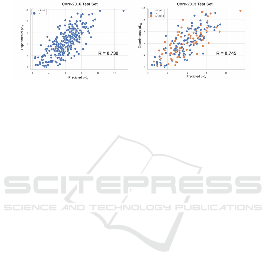
Figure 5: Experiment vs Predicted Binding Affinity in pK
a
for best LigityScore3D model. The left scatter plot represents the
core 2016 set, whilst the right scatter plot represents the core 2013 set.
The scatter plots for the predicted affinity versus
the experimental affinity for best performing Ligi-
tyScore3D model is shown in Figure 5. The scat-
ter plots represent the Core-2016 (left) and the Core-
2013 (right) sets showing good correlation between
predicted and experimental affinities. The ideal model
would produce a plot of function y = x, as the pre-
dicted affinity should be equal to the experimental
value. The ranking of LigityScore for CASF-2013
and CASF-2016 are presented in Tables 3 and 4.
Apart from the scoring function evaluated directly in
CASF, Tables 3 and 4 include other scoring functions,
marked with an asterix (*), that represent results re-
ported in literature (in individual publications) that
also utilise the CASF benchmarks. Tables 3 and 4
thus provide, to the best of our knowledge, a compre-
hensive list of the scoring functions developed in re-
cent years to date, that compare and rank the different
scoring functions available. LigityScore3D achieved
5
th
place in the CASF-2013 benchmark with an av-
erage R-score of 0.713, and exceeds the reported
CASF-2013 score for Pafnucy. On the CASF-2016
benchmark, LigityScore models achieve the 7
th
and
8
th
places.
4 CONCLUSIONS
In this study we explored the use of CNNs to develop
a scoring function, called LigityScore, for binding
affinity prediction. Machine learning scoring func-
tions have been developed to address the limitations
of classical models, such as the use of linear models,
imposed functional form, and their inability to learn
from new data. However, conventional ML based
scoring functions still rely on a degree of feature engi-
neering that requires expert knowledge to preprocess
the data. This, in turn, led to the introduction of deep
learning methods. To this effect we have developed
two different protein-ligand representations that are
extracted directly from the 3D structure of both the
protein and ligand using pharmocophoric features.
The choice of representation of the protein-ligand
structure determines the flexibility and expressiveness
that the model is able to learn and ultimately its scor-
ing power. Although deep learning methods extract
features automatically during training, correct repre-
sentation of the complex is critical for the feature ex-
traction ability of the DL model. As a point for im-
provement for LigityScore performance, future work
would focus on the data representation component of
the protein-ligand complex to build on the existing
representation and possibly seek ways to incorporate
alternate types of features within LigityScore. In this
regard one of the research tasks would be to look into
additional pharmacophoric feature families (or types)
that could help create an enriched descriptor. Other
features such as the spatial distribution count for dis-
tances between key atom combinations could be con-
sidered as another dimension to the LigityScore rep-
resentation. Additionally, since CNNs are difficult to
interpret, in future work we would apply techniques
such as SHAP (Lundberg and Lee, 2017) to determine
critical features used for predictions.
The major contribution for this study is in the pre-
sentation of a novel protein-ligand representation for
use as a CNN scoring function for binding affinity
prediction adapted from Ebejer et al. (2019). Rep-
resentation engineering is required when using CNN
for SBVS as the data needs to represent the protein-
ligand structure. Representation engineering is nec-
essary since the protein-ligand complex cannot be in-
put directly into the CNN as in the case of an im-
age. In our approach we use spatial distances be-
tween key pharmacophoric features which is simpler
than creating a mathematical model to describe the
protein-ligand interactions. LigityScore still relies on
the automatic feature extraction of CNNs for feature
LigityScore: Convolutional Neural Network for Binding-affinity Predictions
47

extraction. Since LigityScore is based on distances
between pharmacophoric features, it also presents a
rotationally invariant representation. Additionally,
the method shows relatively good performance that
marginally exceed the Pafnucy R-score performance
on the CASF-2013 benchmark by 0.01 on average, us-
ing a less computationally complex model that can be
trained 16 times faster. The LigityScore models can
potentially be used for affinity predictions for novel
molecules, and as a scoring function for docking in
virtual screening.
A recent paper by Shen et al. (2020) highlights
the importance of assessing the scoring function in all
four powers (scoring, ranking, docking, and screen-
ing) of the CASF benchmark for a 360 degree per-
formance evaluation. Due to the recent release of
Shen et al. (2020) it was not possible to extend eval-
uation of LigityScore on the rest of the powers. This
is a limitation in the sense that these results are not
known, and future work would consider testing Ligi-
tyScore for the other powers in the CASF benchmark.
Recent literature for deep learning scoring functions
also focused on only the scoring power aspect such as
Stepniewska-Dziubinska et al. (2017), Jim
´
enez et al.
(2018), and Zheng et al. (2019), and therefore a simi-
lar approach was taken. Shen et al. (2020) has shown
that Pafnucy and OnionNet do not perform well on the
rest of the benchmark powers, and even report perfor-
mance lower than the classical functions.
Although the ideal scoring function should per-
form well in all CASF benchmark powers, we argue
that this is not necessarily the case and a particular
ML scoring function may not be suited for every sce-
nario. Therefore a different version, trained for a par-
ticular power, may be better suited. As an example,
the screening power would require the scoring func-
tion model to differentiate between actives and inac-
tives. However, the models trained with the PDB-
bind dataset do not include any inactive information.
Due to the lack of experimentally-validated inactives
there are no evaluation datasets that include inactive
molecules highlighting the need for better and more
complete datasets (Sieg et al., 2019). ML models,
including DL, use learning by representation to ex-
tract the underlying function in the data. If the dataset
does not include the inactive class it is intuitive that
the model may not respond well when presented with
inactive molecules. A ML scoring function can be
developed to cater for the particular power, leverag-
ing on the flexibility they provide to adjust and derive
their parameters from the given training data automat-
ically.
Finding a suitable representation of the protein-
ligand complex is a major challenge when building a
scoring function, and is key for accurate predictions
using deep learning techniques. In our work we have
successfully found a suitable representation that to the
best of our knowledge was never used for binding
affinity prediction, which provides good results and
ranked 5
th
in the CASF-2013 benchmark. Therefore,
although our work did not outperform the top scoring
function we deem it is still a valid contribution to the
area and may be further enhanced in future work, or
may also serve as motivation and inspiration for other
researchers to seek out alternative methods that in-
crease the effectiveness of scoring functions and vir-
tual screening in general.
We believe a deeper understanding of CNN in the
domain of SBVS is still required, and a breakthrough
like the work of Krizhevsky et al. (2012) in the com-
puter vision domain is still being sought after in this
challenging domain. Nonetheless, we also believe
that ML and DL techniques will lead the future of the
development of scoring functions.
ACKNOWLEDGEMENTS
We would like to thank the AWS Research Credits
Team for supporting our research with AWS credits
to develop our models.
REFERENCES
Ain, Q. U., Aleksandrova, A., Roessler, F. D., and Ballester,
P. J. (2015). Machine-learning scoring functions to
improve structure-based binding affinity prediction
and virtual screening. Wiley Interdisciplinary Re-
views: Computational Molecular Science, 5(6):405–
424.
Berman, H., Henrick, K., and Nakamura, H. (2003). An-
nouncing the worldwide protein data bank. Nature
Structural & Molecular Biology, 10(12):980–980.
Boyles, F., Deane, C. M., and Morris, G. M. (2020). Learn-
ing from the ligand: using ligand-based features to
improve binding affinity prediction. Bioinformatics,
36(3):758–764.
Ching, T., Himmelstein, D. S., Beaulieu-Jones, B. K.,
Kalinin, A. A., Do, B. T., Way, G. P., Ferrero, E.,
Agapow, P.-M., Zietz, M., Hoffman, M. M., et al.
(2018). Opportunities and obstacles for deep learn-
ing in biology and medicine. Journal of The Royal
Society Interface, 15(141):20170387.
Goldberg, Y. (2016). A primer on neural network models
for natural language processing. Journal of Artificial
Intelligence Research, 57:345–420.
He, K., Zhang, X., Ren, S., and Sun, J. (2015). Delving
deep into rectifiers: Surpassing human-level perfor-
mance on imagenet classification. In 2015 IEEE In-
BIOINFORMATICS 2021 - 12th International Conference on Bioinformatics Models, Methods and Algorithms
48

ternational Conference on Computer Vision (ICCV),
pages 1026–1034.
Jim
´
enez, J., Skalic, M., Martinez-Rosell, G., and De Fabri-
tiis, G. (2018). K deep: protein–ligand absolute bind-
ing affinity prediction via 3d-convolutional neural net-
works. Journal of chemical information and model-
ing, 58(2):287–296.
Kaggle, M. (2012). Kaggle: Merck molecular activity chal-
lenge. https://www.kaggle.com/c/MerckActivity, Ac-
cessed Feb 8, 2019.
Kingma, D. P. and Ba, J. (2014). Adam: A
method for stochastic optimization. cite
arxiv:1412.6980Comment: Published as a con-
ference paper at the 3rd International Conference for
Learning Representations, San Diego, 2015.
Landrum, G. (2020). Rdkit: Open-source cheminformatics.
Accessed April, 2020.
Leach, A. R., Gillet, V. J., Lewis, R. A., and Taylor, R.
(2010). Three-dimensional pharmacophore methods
in drug discovery. Journal of medicinal chemistry,
53(2):539–558.
LeCun, Y., Bengio, Y., and Hinton, G. (2015). Deep learn-
ing. nature, 521(7553):436–444.
Li, Y., Liu, Z., Li, J., Han, L., Liu, J., Zhao, Z., and Wang,
R. (2014). Comparative assessment of scoring func-
tions on an updated benchmark: 1. compilation of the
test set. Journal of chemical information and model-
ing, 54(6):1700–1716.
Liu, Z., Cui, Y., Xiong, Z., Nasiri, A., Zhang, A., and
Hu, J. (2019). Deepseqpan, a novel deep convolu-
tional neural network model for pan-specific class i
hla-peptide binding affinity prediction. Scientific re-
ports, 9(1):794.
Liu, Z., Su, M., Han, L., Liu, J., Yang, Q., Li, Y., and
Wang, R. (2017a). Forging the basis for developing
protein–ligand interaction scoring functions. Accounts
of chemical research, 50(2):302–309.
Liu, Z., Su, M., Han, L., Liu, J., Yang, Q., Li, Y., and
Wang, R. (2017b). Forging the basis for developing
protein–ligand interaction scoring functions. Accounts
of chemical research, 50(2):302–309.
Lundberg, S. M. and Lee, S.-I. (2017). A unified approach
to interpreting model predictions. In Advances in Neu-
ral Information Processing Systems 30, pages 4765–
4774. Curran Associates, Inc.
Nguyen, D. D. and Wei, G.-W. (2019a). Agl-score: Al-
gebraic graph learning score for protein–ligand bind-
ing scoring, ranking, docking, and screening. Journal
of chemical information and modeling, 59(7):3291–
3304.
Nguyen, D. D. and Wei, G.-W. (2019b). Dg-gl: Differen-
tial geometry-based geometric learning of molecular
datasets. International journal for numerical methods
in biomedical engineering, 35(3):e3179.
¨
Ozt
¨
urk, H.,
¨
Ozg
¨
ur, A., and Ozkirimli, E. (2018). Deepdta:
deep drug–target binding affinity prediction. Bioinfor-
matics, 34(17):i821–i829.
Paszke, A., Gross, S., Massa, F., Lerer, A., Bradbury, J.,
Chanan, G., Killeen, T., Lin, Z., Gimelshein, N.,
Antiga, L., Desmaison, A., Kopf, A., Yang, E., De-
Vito, Z., Raison, M., Tejani, A., Chilamkurthy, S.,
Steiner, B., Fang, L., Bai, J., and Chintala, S. (2019).
Pytorch: An imperative style, high-performance deep
learning library. In Advances in Neural Information
Processing Systems 32, pages 8024–8035. Curran As-
sociates, Inc.
P
´
erez-Sianes, J., P
´
erez-S
´
anchez, H., and D
´
ıaz, F. (2019).
Virtual screening meets deep learning. Current
computer-aided drug design, 15(1):6–28.
Ragoza, M., Hochuli, J., Idrobo, E., Sunseri, J., and Koes,
D. R. (2017). Protein–ligand scoring with convolu-
tional neural networks. Journal of chemical informa-
tion and modeling, 57(4):942–957.
Rifaioglu, A. S., Atas, H., Martin, M. J., Cetin-Atalay, R.,
Atalay, V., and Dogan, T. (2018). Recent applications
of deep learning and machine intelligence on in silico
drug discovery: methods, tools and databases. Brief.
Bioinform, 10.
Sieg, J., Flachsenberg, F., and Rarey, M. (2019). In need
of bias control: Evaluating chemical data for machine
learning in structure-based virtual screening. Jour-
nal of chemical information and modeling, 59(3):947–
961.
Stepniewska-Dziubinska, M. M., Zielenkiewicz, P., and
Siedlecki, P. (2017). Pafnucy–a deep neural network
for structure-based drug discovery. stat, 1050:19.
Su, M., Yang, Q., Du, Y., Feng, G., Liu, Z., Li, Y., and
Wang, R. (2018). Comparative assessment of scoring
functions: the casf-2016 update. Journal of chemical
information and modeling, 59(2):895–913.
Szegedy, C., Liu, W., Jia, Y., Sermanet, P., Reed, S.,
Anguelov, D., Erhan, D., Vanhoucke, V., and Rabi-
novich, A. (2015). Going deeper with convolutions.
In Proceedings of the IEEE conference on computer
vision and pattern recognition, pages 1–9.
Tompson, J., Goroshin, R., Jain, A., LeCun, Y., and Bregler,
C. (2015). Efficient object localization using convo-
lutional networks. In Proceedings of the IEEE Con-
ference on Computer Vision and Pattern Recognition,
pages 648–656.
Ulyanov, D., Vedaldi, A., and Lempitsky, V. (2017). Im-
proved texture networks: Maximizing quality and di-
versity in feed-forward stylization and texture synthe-
sis. In The IEEE Conference on Computer Vision and
Pattern Recognition (CVPR). IEEE.
W
´
ojcikowski, M., Kukiełka, M., Stepniewska-Dziubinska,
M. M., and Siedlecki, P. (2019). Development of
a protein–ligand extended connectivity (plec) finger-
print and its application for binding affinity predic-
tions. Bioinformatics, 35(8):1334–1341.
Zhang, H., Liao, L., Saravanan, K. M., Yin, P., and Wei,
Y. (2019). Deepbindrg: a deep learning based method
for estimating effective protein–ligand affinity. PeerJ,
7:e7362.
Zheng, L., Fan, J., and Mu, Y. (2019). Onionnet: a multiple-
layer intermolecular-contact-based convolutional neu-
ral network for protein–ligand binding affinity predic-
tion. ACS omega, 4(14):15956–15965.
LigityScore: Convolutional Neural Network for Binding-affinity Predictions
49
