MetaBox+: A New Region based Active Learning Method for Semantic

Segmentation using Priority Maps

Pascal Colling

1,2

, Lutz Roese-Koerner

, Hanno Gottschalk

and Matthias Rottmann

University of Wuppertal, School of Mathematics and Natural Sciences, IMACM & IZMD, Germany

Aptiv, Wuppertal, Germany

Keywords:

Active Learning, Semantic Segmentation, Priority Maps via Meta Regression, Cost Estimation.

Abstract:

We present a novel region based active learning method for semantic image segmentation, called MetaBox+.

For acquisition, we train a meta regression model to estimate the segment-wise Intersection over Union (IoU)

of each predicted segment of unlabeled images. This can be understood as an estimation of segment-wise

prediction quality. Queried regions are supposed to minimize to competing targets, i.e., low predicted IoU

values / segmentation quality and low estimated annotation costs. For estimating the latter we propose a sim-

ple but practical method for annotation cost estimation. We compare our method to entropy based methods,

where we consider the entropy as uncertainty of the prediction. The comparison and analysis of the results

provide insights into annotation costs as well as robustness and variance of the methods. Numerical exper-

iments conducted with two different networks on the Cityscapes dataset clearly demonstrate a reduction of

annotation effort compared to random acquisition. Noteworthily, we achieve 95% of the mean Intersection

over Union (mIoU), using MetaBox+ compared to when training with the full dataset, with only 10.47% /

32.01% annotation effort for the two networks, respectively.

1 INTRODUCTION

In recent years, semantic segmentation, the pixel-

wise classiﬁcation of the semantic content of im-

ages, has become a standard method to solve prob-

lems in image and scene understanding. Examples

of applications are autonomous driving and environ-

ment understanding (Zhao et al., 2017), (Chen et al.,

2018), (Wang et al., 2019), biomedical analyses (Ron-

neberger et al., 2015) and further computer visions

tasks. Deep convolutional neural networks (CNN) are

commonly used in semantic segmentation. In order to

maximize the accuracy of a CNN, a large amount of

annotated and varying data is required, since with an

increasing number of samples the accuracy increases

only logarithmically (Sun et al., 2017). For instance

in the ﬁeld of autonomous driving, fully and precisely

annotated street scenes require an enormous (and tir-

ing) annotation effort. Also biomedical applications,

in general domains that require expert knowledge for

annotation, suffer from high annotation costs. Hence,

from multiple perspectives (annotation) cost reduc-

tion while maintaining model performance is highly

desirable.

agg

Init

Candiate

Boxes

Dataset

CNN

Priority

Maps

Aggregation Joining

M UL

Oracle

Prediction

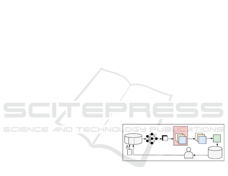
Figure 1: Illustration of the region based AL method. The

red parts highlight the novel meta regression based ingredi-

ents: as query priority maps we use MetaSeg and the esti-

mated number of clicks. Training of MetaSeg requires an

additional small sample of data (ﬁxed for the whole course

of AL), indicated by M ⊂ P (in red color).

One possible approach is active learning (AL),

which basically consists of alternatingly annotating

data and training a model with the currently available

annotations. The key component in this algorithm that

can substantially leverage the learning process is the

so called query or acquisition strategy. The ultimate

goal is to label the data that leverages the model per-

formance most while paying with as small labeling

costs as possible. For an introduction to AL methods,

see e.g. (Settles, 2009).

First AL approaches (before the deep learning

(DL) era) for semantic segmentation, for instance

Colling, P., Roese-Koerner, L., Gottschalk, H. and Rottmann, M.

MetaBox+: A New Region based Active Learning Method for Semantic Segmentation using Priority Maps.

DOI: 10.5220/0010227500510062

In Proceedings of the 10th International Conference on Pattern Recognition Applications and Methods (ICPRAM 2021), pages 51-62

ISBN: 978-989-758-486-2

FCN8

Deeplab

RandomBoxMetaBox+Full setGround Truth

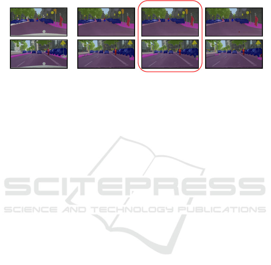
Figure 2: Segmentation results with our novel method MetaBox+ for two CNN models. With an annotation effort of only

10.47% for the Deeplab model (top) and 32.01% for the FCN8 model (bottom), we achieve 95% full set mIoU. Additionally,

the segmentation results are shown when training the networks with the full dataset (Full set) and with a random selection

strategy (RandomBox) producing the same annotation effort as MetaBox+. Annotation effort is stated in terms of a click

based metric (cost

, Equation (10)).

based on conditional random ﬁelds, go back to (Vezh-

nevets et al., 2012), (Konyushkova et al., 2015), (Jain

and Grauman, 2016), (Mosinska et al., 2017). At the

heart of an AL method is the so-called query strat-

egy that decides which data to present to the anno-

tator / oracle next. In general, uncertainty sampling

is one of the most common query strategies (Wang

et al., 2016), (Gal et al., 2017), (Beluch et al., 2018),

(Rottmann et al., 2018), (Hahn et al., 2019), besides

that there also exist approaches on expected model

change (Vezhnevets et al., 2012) and reinforcement

learning based AL (Casanova et al., 2020).

In recent years, approaches to deep AL for seman-

tic segmentation have been introduced, primarily for

two applications, i.e., biomedical image segmenta-

tion and semantic street scene segmentation. The ap-

proaches in (Yang et al., 2017), (Gorriz et al., 2017),

(Özdemir et al., 2018), (Mahapatra et al., 2018)

are speciﬁcally designed for medical and biomed-

ical applications, mostly focusing on foreground-

background segmentation. Due to the underlying na-

ture of the data, these approaches refer to annotation

costs in terms of the number of labeled images.

The methods presented in (Mackowiak et al.,

2018), (Siddiqui et al., 2019), (Kasarla et al., 2019),

(Casanova et al., 2020) use region based proposals.

All of them evaluate the model accuracy in terms of

mean Intersection over Union (mIoU). The method

in (Siddiqui et al., 2019) is designed for multi-view

semantic segmentation datasets, in which objects are

observed from multiple viewpoints. The authors in-

troduce two new uncertainty based metrics and aggre-

gate them on superpixel (SP) level (SPs can be viewed

as visually uniform clusters of pixels). They measure

the costs by the number of labeled pixels. Further-

more they have shown that labeling on SP level can

reduce the annotation time by 25%. In (Kasarla et al.,

2019) a new uncertainty metric on SP level is deﬁned,

which includes the information of the Shannon En-

tropy (Shannon, 2001), combined with information

about the contours in the original image and a class-

similarity metric to put emphasis on rare classes. In

(Kasarla et al., 2019), the number of pixels labeled

deﬁne the costs. The authors of (Casanova et al.,

2020) utilize the same cost metric. The latter work

uses reinforcement learning to ﬁnd the most infor-

mative regions, which are given in quadratic format

of ﬁxed size. This procedure aims at ﬁnding regions

containing instances of rare classes. The method in

(Mackowiak et al., 2018) queries quadratic regions

of ﬁxed-size from images as well. In contrast to the

methods discussed before, the costs are measured by

annotation clicks. They use a combination of un-

certainty measure (Vote (Dagan and Engelson, 1995)

and Shannon Entropy) and a clicks-per-polygon based

cost estimation, which is regressed by a second DL

model. The methods in (Mackowiak et al., 2018),

(Kasarla et al., 2019), (Casanova et al., 2020) are fo-

cusing on multi-class semantic segmentation dataset

like Cityscapes (Cordts et al., 2016).

In this work, we introduce a query strategy, which

is based on an estimation of the segmentation qual-

ity. We use the meta regression method MetaSeg,

introduced in (Rottmann et al., 2020), to predict the

segment-wise IoU and extend this method by aggre-

gating the segment-wise IoU over the quadratic can-

didate regions of images. MetaSeg was further ex-

tended in other directions, i.e., for controlled false-

negative reduction (Chan et al., 2020), for time-

dynamic uncertainty estimates of videos (Maag et al.,

2020) as well as for taking resolution-dependent

uncertainties into account (Rottmann and Schubert,

2019).

In semantic segmentation, the annotation cost de-

pends less on the number of labeled pixels, but rather

on the complexity of labeled contours. The latter are

ICPRAM 2021 - 10th International Conference on Pattern Recognition Applications and Methods

typically approximated by polygons where polygon

nodes correspond to clicks. To this end, we intro-

duce a simple and practical method to estimate an-

notation costs in terms of clicks. Through the com-

bination of both, we target informative regions with

low annotation costs. A sketch of our method is

given in Figure 1. Based on the number of clicks re-

quired for annotation, we introduce a new cost met-

ric, since we are also evaluating the costs in terms of

clicks and not in terms of labeled images or pixels.

For numerical experiments we used the Cityscapes

dataset (Cordts et al., 2016) with two models, namely

the FCN8 (Long et al., 2015) and the Deeplabv3+

Xcpetion65 (Chen et al., 2018) (following in short

only Deeplab).

2 RELATED WORK

In this section, we compare our work to the works

closest to ours. Therefore, we focus on the region

based approaches (Mackowiak et al., 2018), (Kasarla

et al., 2019), (Siddiqui et al., 2019), (Casanova et al.,

2020). All of them evaluate the model accuracy in

terms of mIoU. The approaches in (Kasarla et al.,

2019), (Siddiqui et al., 2019) use handcrafted uncer-

tainty metrics aggregated on SP level and also query

regions in form of SP. While (Siddiqui et al., 2019) is

speciﬁcally designed for multi-views datasets, our ap-

proach focuses on single-view multi-class segmenta-

tion of street scenes. For the query strategy presented

in (Kasarla et al., 2019), the authors do not only use

uncertainty metrics, but also information about the

contours of the images as well as class similarities

of the SP to identify rare classes. We also use dif-

ferent types of information to generate our proposals.

The AL method in (Casanova et al., 2020) is based

on deep reinforcement learning and queries quadratic

ﬁxed size regions. The only similarity to our approach

is the format of the queried regions. Compared to

the approaches above (Kasarla et al., 2019), (Siddiqui

et al., 2019), (Casanova et al., 2020) we do not focus

on ﬁnding a minimal dataset to achieve a satisfying

model accuracy. We consider the costs in terms of

required clicks for annotating a region and aim to re-

duce the human annotation effort (therefore we refer

to those clicks as costs). To this extent, we take an es-

timation of the labeling effort during acquisition into

account. In addition, we estimate the segmentation

quality to identify regions of interest.

As in (Mackowiak et al., 2018), our candidate re-

gions for acquisition are square-shaped and of ﬁxed

size, and we also use a cost metric based on the num-

ber of clicks required to draw a polygon overlay for

an object. Hence, (Mackowiak et al., 2018) is in spirit

closest to our work. However, instead of using an un-

certainty measure to identify high informational re-

gions, we use information about the estimated seg-

mentation quality in terms of the segment-wise Inter-

section over Union (IoU) (see (Rottmann et al., 2020),

(Jaccard, 1912)). Entropy is a common measure to

quantify uncertainty. However, in semantic segmen-

tation we observe increased uncertainty on segment

boundaries, while uncertainty in the interior is often

low. This is in line with the observation that, neu-

ral network in general provide overconﬁdent predic-

tions (Goodfellow et al., 2014), (Hein et al., 2019).

We solve this problem by evaluating the segmentation

quality of whole predicted segments.

Furthermore, also our cost estimation method dif-

fers substantially from the one presented in (Mack-

owiak et al., 2018). While the authors of (Mackowiak

et al., 2018) use another CNN to regress on the num-

ber of clicks per candidate region, we infer an esti-

mate of the number of required clicks directly from

the prediction on the segmentation network and show

in our results, that our measure is indeed strongly cor-

related with the true number of clicks per candidate

region.

3 REGION BASED ACTIVE

LEARNING

In this section we ﬁrst describe a region based AL

method, which queries ﬁxed-size and quadratic im-

age regions. Afterwards, we describe our new AL

method. This method is subdivided into a 2-step pro-

cess: ﬁrst, we predict the segmentation quality by

using the segment-wise meta regression method pro-

posed in (Rottmann et al., 2020). Second, we incor-

porate a cost estimation of the click number required

to label a region, we term this add on.

3.1 Method Description

For the AL method we assume a CNN as semantic

segmentation model with pixel-wise softmax proba-

bilities as output. The corresponding segmentation

mask, also called segmentation, is the pixel-wise ap-

plication of the argmax function to the softmax prob-

abilities. The dataset is given as data pool P . The

set of all labeled data is denoted by L and set of unla-

beled data by U. At the beginning we have no labeled

data, i.e., L =

0, and we wish to provide labels over a

given number of classes c ∈ N,c ≥ 2 for all images.

A generic AL method can be summarized as follows:

Initially, a small set of data from U is labeled and

MetaBox+: A New Region based Active Learning Method for Semantic Segmentation using Priority Maps

added to L. Then, two steps are executed alternat-

ingly in a loop. Firstly, the model (the CNN) is trained

on L. Thereafter, a chosen amount of unlabeled data

from U is queried according to a query strategy, la-

beled and added to L.

In region based AL, we add newly labeled regions

to L instead of whole images. An image x remains in

U as long as it is not entirely labeled. In order to avoid

multiple queries of the same region, a region that is

contained in both U and L is tagged with a query

priority equal to zero. In the remainder of this section,

we describe the query function in detail and introduce

an appropriate concept of priority in the given context.

Region based Queries. The query strategy is a

key ingredient of an AL method. In general, most

query function designs strive for maximally leverag-

ing training progress (i.e., achieving high validation

accuracy after short time) at reduced labeling costs.

Thus, we aim at querying regions of images which

leads to a region-wise concept of query priority.

In what follows, we only compute measures of

priority by means of the softmax output of the neu-

ral network. To this end, let

f : [0,1]

w×h×3

→ [0,1]

w×h×c

(1)

be a function given by a segmentation network pro-

viding softmax probabilities for a given input image,

where w denotes the image width, h the height and c

the number of classes.

A priority map can be viewed as another function

g : [0,1]

w×h×c

→ [0,1]

w×h

(2)

that outputs one priority score per image pixel. The

output of g can be viewed as a heatmap that indicates

priority. A higher score of priority should presumably

correlate with the attractiveness of the corresponding

ground truth. A typical example for g is the pixel-wise

entropy H which for a chosen pixel (i, j) is given by

H(y

i, j,·

) = −

∑

k=1

i, j,c

log(y

i, j,c

) (3)

where y

i, j,c

= f (x)

i, j,c

∈ [0,1] for a given input x ∈

[0,1]

w×h×3

. The priority maps that we use in our

method are introduced in the subsequent section.

Note that, if an image pixel has already been labeled,

we overwrite the corresponding pixel value of the pri-

ority map by zero.

Our AL method queries regions that are square-

shaped (boxes) and of ﬁxed width b ∈ N. A box-wise

overall priority score is obtained via aggregation. To

this end, we simply choose to sum up the scores. That

is, given a box B ⊂ [0,1]

w×h

, the aggregated score

given by

agg

(y,B) =

∑

(i, j)∈B

i, j

(y). (4)

Given the set B of all possible boxes of width b in

[0,1]

w×h

, we can deﬁne an aggregated priority map

(y) = {g

agg

(y,B) : B ∈ B} (5)

which can be viewed as another heatmap resulting

from a convolution operation with a constant ﬁlter.

Given t aggregated priority scores, for the sake of

brevity named h

(1)

(y,B),...,h

(t)

(y,B), we deﬁne a

joint priority score by

h(y,B) =

∏

s=1

(s)

(y,B). (6)

Analogously to Equation (5) we introduce a joint pri-

ority map h

(y). However, in what follows we do not

distinguish between joint priority maps and singleton

(aggregated) priority maps as this follows from the

context. Furthermore, we only refer to priority maps

while performing calculations on priority score level.

Algorithm. In summary, our AL method proceeds

as follows. Initially, a randomly chosen set of m

init

entire images from U is labeled and then moved to

L. Afterwards, the AL method proceeds as previously

described in the introduction of this section. Deﬁning

the set of all candidate boxes as

C = {(y,B) : y = f (x), x ∈ U, B ∈ B }, (7)

we query in each iteration a chosen number m

of non-overlapping boxes Q = {(y

) : j =

1,...m

} ⊂ C, with the highest scores h(y,B), i.e.,

(y,B) ∈ Q, (y

) /∈ Q (8)

=⇒ h(y, B) ≥ h(y,B

) or (B ∩ B

0 and y = y

A sketch of the whole AL loop is depicted by Fig-

ure 1.

3.2 Joint Priority Maps based on Meta

Regression and Click Estimation

It remains to specify the priority maps h

(i)

(y,B) de-

ﬁned in the previous section. In our method, we have

t = 2 priority maps. As an estimate of prediction qual-

ity, we use MetaSeg (Rottmann et al., 2020) which

provides a quality estimate in [0,1] for each segment

predicted by f . This aims at querying ground truth for

image regions that presumably have been predicted

badly. Mapping predicted qualities back to each pixel

of a given segment and thereafter aggregating the val-

ues over boxes, we obtain our ﬁrst priority map h

(1)

ICPRAM 2021 - 10th International Conference on Pattern Recognition Applications and Methods

On the other hand, we wish to label regions that are

easy (or cheap) to label. Therefore, we estimate the

number of clicks required to annotate a box B. From

this, we deﬁne another priority map h

(2)

which con-

tains high values for regions with low estimated num-

bers of clicks and vice versa (details follow in the up-

coming paragraphs). We query boxes according to the

product of priorities, i.e.,

h(y,B) = h

(1)

(y,B) · h

(2)

(y,B) (9)

as being done in (Mackowiak et al., 2018), but with

both h

(1)

and h

(2)

being different. In what follows,

we describe the priority maps g

(1)

(y) and g

(2)

(y)

more precisely, where the aggregated priority maps

(1)

(y,B) and h

(2)

(y,B) are constructed as in Sec-

tion 3.1.

Priority via MetaSeg. As priority map g

(1)

(y) we

use MetaSeg (Rottmann et al., 2020) which estimates

the segmentation quality by means of predicting the

IoU of each predicted segment with the ground truth.

MetaSeg uses regression models with different

types of hand-crafted input metrics. These include

pixel-wise dispersion measures like (Shannon) en-

tropy and the difference between the two largest soft-

max probabilities. These pixel-wise dispersions are

aggregated on segment level by computing the mean

over each segment. Here, a segment is a connected

component of a predicted segmentation mask of a

given class.

In addition, for each predicted segment we con-

sider shape-related quantities, i.e., the segment size,

the fractality and the surface center of mass coordi-

nates. Furthermore, averaged class probabilities for

each predicted segment are presented to the regres-

sion model.

Training the regression model of MetaSeg re-

quires ground truth to compute the IoU for each pre-

dicted segment and the corresponding ground truth

segment. Since the prediction changes in every itera-

tion of the AL method, we train the regression model

for MetaSeg once in every AL iteration. In order to

have ground truth available for training the regression

model, we randomly select and label a further initial

dataset M of n

meta

samples, which will be ﬁxed for

the whole AL process. To predict the quality of net-

work predictions via MetaSeg, we perform the fol-

lowing steps after updating the semantic segmentation

model:

1. Infer the current CNN’s predictions for all images

in M ,

2. Compute the metrics for each predicted segment

(from step 1.),

3. Train MetaSeg to predict the IoU by means of the

metrics from step 2.

4. Infer the current CNN’s predictions for the unla-

beled data U,

5. Compute the metrics for each predicted segment

that belongs to U (as in step 2.),

6. Apply MetaSeg in inference mode to each pre-

dicted segment from U (from step 4.) and its met-

rics (from step 5.) to predict the IoU.

For each unlabeled (i.e., not entirely labeled)

image, MetaSeg provides a segmentation quality

heatmap q(y) by registering the predicted IoU val-

ues of the predicted segments for each of their cor-

responding pixels. An example of the segmentation

quality heatmap is given in Figure 3. The corre-

sponding priority map as deﬁned in Equation (2), is

obtained via g

(1)

(y) = 1 − q(y). Hence, regions of

(1)

(y) containing relatively high values are consid-

ered as being attractive for acquisition. More details

on MetaSeg can be found in (Rottmann et al., 2020).

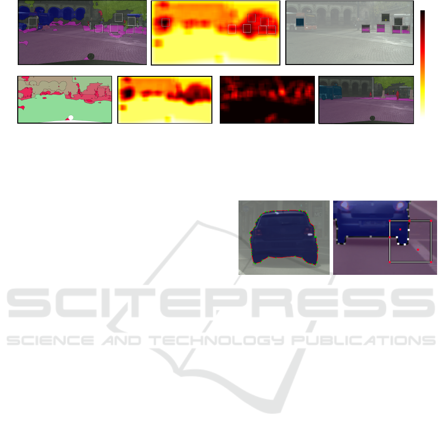
Figure 3: Prediction of the IoU values. The ﬁgure consists

of ground truth (bottom left), predicted segments (bottom

right), true IoU for the predicted segments (top left) and

predicted IoU for the predicted segments (top right). In the

top row, green color corresponds to high IoU values and red

color to low ones, for the white regions there is no ground

truth available.

Priority via Estimated Number of Clicks. As an

additional priority map g

(2)

(y) we choose an esti-

mate of annotation costs. Multi-class semantic seg-

mentation datasets are generally labeled with a poly-

gon based annotation tool, i.e., the objects are de-

scribed by a ﬁnite number of vertices connected by

edges such that the latter form a closed loop. (Cordts

et al., 2016), (Neuhold et al., 2017). If the ground

truth is given only pixel-wise, an estimate of the num-

ber of required clicks can be approximated by ap-

plying the Ramer-Douglas-Peucker (RDP) algorithm

(Ramer, 1972), (Douglas and Peucker, 1973) to the

segmentation contours.

To estimate the true number of clicks required for

annotation in the AL process, we correlate this num-

ber with how many clicks it approximately requires

MetaBox+: A New Region based Active Learning Method for Semantic Segmentation using Priority Maps

to annotate the predicted segmentation (provided by

the current CNN) using the RDP algorithm. The ap-

proximation accuracy of the RDP algorithm is con-

trolled by a parameter ε. We deﬁne a cost map κ(y)

via κ

i, j

(y) = 1 if there is a polygon vertex in pixel

(i, j) and κ

i, j

(y) = 0 else. Since we are prioritising

regions with low estimated costs, the priority map is

given by g

(2)

(y) = 1 − κ(y). Following the construc-

tion in Section 3.1 yields the aggregated priority map

(2)

(y,B). A visual example of the cost estimation is

given in Figure 5 (left panel).

In our tests with the RDP algorithm applied to

ground truth segmentations, we observed that on av-

erage the estimated number of click is fairly close to

the true number of clicks provided by the Cityscapes

dataset. Therefore, if we assume that over the course

of AL iterations, the model performance increases,

approaching a level of segmentation quality that is

close to ground truth, then the described cost estima-

tion on average will approach the click numbers in the

ground truth.

In the following, we distinguish between the fol-

lowing methods: MetaBox uses only the priority via

MetaSeg and MetaBox+ uses both the joint priority

of MetaSeg and the estimated number of clicks. An

overview of the different steps of our AL method is

given by Figure 1 and an exemplary visualization of

the different stages of MetaBox+ is shown in Figure 4.

Note that there are different conventions for counting

clicks which we discuss in Section 4.1.

Further Priority Maps and Baseline Methods.

For the sake of comparison, we also deﬁne a prior-

ity map based on the pixel-wise entropy as in Equa-

tion (3). Analogously to MetaBox and MetaBox+, we

introduce EntropyBox and EntropyBox+: Entropy-

Box uses only the priority via entropy and Entropy-

Box+ uses the joint priority of the entropy and the

estimated number of clicks. The method Entropy-

Box+ is similar to the method introduced in (Mack-

owiak et al., 2018). The corresponding authors also

use a combination of the entropy and a cost estima-

tion, but the cost estimation is computed by a second

DL model. Furthermore, as a naive baseline we con-

sider a random query function that performs queries

by means of random priority maps. We term this

method RandomBox.

4 EXPERIMENTS

Before presenting results of our experiments, we in-

troduce metrics to measure the annotation effort. To

this end, we discuss different types of clicks required

for labeling and how they can be taken into account

for deﬁning annotation costs. Afterwards we specify

the experiments settings and the implementation de-

tails. Thereafter, we present numerical experiments

where we compare different query strategies with re-

spect to performance and robustness. Furthermore we

study the impact of incorporating annotation cost es-

timations.

4.1 Measuring Annotation Effort

In semantic segmentation, annotation is usually gen-

erated with a polygon based annotation tool. A con-

nected component of a given class is therefore repre-

sented by a polygon, i.e., a closed path of edges. This

path is constructed by a human labeler clicking at the

corresponding vertices. We term these vertices poly-

gon clicks c

∈ N. Since we query quadratic image re-

gions (boxes), we introduce the following additional

types of clicks:

• intersection clicks, c

(B) ∈ N

, occur due to the

intersection between the contours of a segment

and the box boundary,

• box clicks, c

(B) ∈ N

, specify the quadratic box

itself,

• class clicks, c

(B) ∈ N, specify the class of the

annotated segment.

For an annotated image, the class clicks correspond

to the number of segments. Like the polygon clicks,

they can also be considered for the cost evaluation of

fully annotated images.

For the evaluation of a dataset P (with fully la-

beled images), c

(P ) ∈ N is the total number of poly-

gon clicks and c

(P ) ∈ N the total number of class

clicks. Let L

be the the initially annotated dataset

(with fully labeled images) and Q the set of all queried

and annotated boxes, then we deﬁne the cost metrics

cost

) + c

(Q) + c

(Q)

(P ) + c

(P )

(10)

cost

) + c

(Q) + c

(Q)

(P )

(11)

with c

]

(Q) =

∑

∈Q

]

), ] ∈ {p, i, b, c}.

In addition to that,

cost

(12)

deﬁnes the costs as amount of labeled pixels with re-

spect to the whole dataset.

The amount of required clicks depends on the annota-

tion tool. The box clicks c

(B) are not necessarily re-

quired: with a suitable tool, the chosen image regions

ICPRAM 2021 - 10th International Conference on Pattern Recognition Applications and Methods

(1) segmentation (2) joined priority map

(3) annotation

(1a) predicted IoU values with MetaSeg

(2a) priority via MetaSeg

(2b) priority via estimated number of clicks

(3a) ground truth

high

low

Figure 4: Visualisation of our AL method MetaBox+ at a speciﬁc AL iteration. The top row shows the segmentation (1),

the joined priority map (2) and the acquired annotation (3). The joined priority map (2) is based on the priority via MetaSeg

(2a) and the estimated number of clicks (2b). High values represent prioritized regions for labeling: in (2b) regions with

low predicted IoU values are of interest in (2b) regions with low estimated clicks. (1a) shows the predicted IoU values via

MetaSeg.

(boxes) are suggested and the annotation process re-

stricted accordingly. Required are the polygon clicks

(B) and the intersections clicks c

(B) to deﬁne the

segment contours as well as the class clicks c

(B) to

deﬁne the class of the annotated segment. Cost metric

cost

(Equation (10)) is based on this consideration.

Cost metric cost

(Equation (11)) is introduced in

(Mackowiak et al., 2018). Due to a personal corre-

spondence with the authors we are able to state details

that go beyond the description provided in (Mack-

owiak et al., 2018): Cost metric cost

is mostly in

accordance with cost

, except for two changes. The

box clicks c

(B) = 4 are taken into account while

the class clicks c

(B) are omitted. Theoretically both

metrics can become greater than 1. Firstly, fully la-

beled images do not require intersection clicks c

Secondly, ground truth segments that are labeled by

more than one box produce multiple class clicks c

to specify the class. In the following, the cost met-

rics cost

, cost

are given in percent (of the

costs for labeling the full dataset without considering

regions). An illustration of the click types is shown in

Figure 5 (right panel).

4.2 Experiment Settings

For our experiments, we used the Cityscapes (Cordts

et al., 2016) dataset. It contains images of urban street

scenes with 19 classes for the task of semantic seg-

mentation. Furthermore, the annotation clicks / poly-

gons are given. We used the training set with 2,975

samples as data pool P . For all model and experiment

evaluations we used the validation set containing 500

samples. We used two CNN models: FCN8 (Long

et al., 2015) (with width multiplier 0.25 introduced in

(Sandler et al., 2018)) and Deeplabv3+ (Chen et al.,

2018) with an Xception65 (Chollet, 2017) backbone,

Figure 5: (left): Visualization of the estimated annotation

clicks obtained by the RDP algorithm applied to the seg-

mentation contours of a predicted segment of class “car”.

The segment contours are highlighted by red color, the

obtained vertices (estimated clicks) are highlighted green.

(right): Example of possible types of clicks we can take into

account for a cost deﬁnition. The white (and gray) pixels

depict true annotation clicks obtained from the data of (here

5 polygon clicks within the box). The red ones represent

additional types of clicks: the ones required for annotating

intersection points of segment contour and box edges (here

2 intersection clicks), the ones for deﬁning the box itself (4

box clicks, one for each corner) and one click per segment

to specify the class of the segment (here 2 class clicks: for

car and street).

(short: Deeplab). Using all training data, also referred

to as full set, we achieve a mIoU of 60.50% on the

validation dataset with the FCN8 model and a mIoU

of 76.11% for the Deeplab model. We have not re-

sized the images, i.e., we used the original resolution

of height h = 1,024 and width w = 2,048. In each

AL iteration, we train the model from scratch. The

training is stopped, if no improvement in term of val-

idation mIoU is achieved over 10 consecutive epochs.

Details regarding the training parameters are given in

Section 4.3 below. All experiments started from an

initial dataset of 50 samples. For experiments with

MetaSeg based queries (MetaBox, MetaBox+), we

took 30 additional samples to train MetaSeg. In each

AL iteration we queried 6,400 boxes with a width of

b = 128, which corresponds to 50 full images in terms

MetaBox+: A New Region based Active Learning Method for Semantic Segmentation using Priority Maps

of the number of pixels.

Each experiment was repeated three times. For

each method we present the mean over the mIoU and

the mean over the cost metrics (cost

, cost

)

of each AL iteration. All CNN trainings were per-

formed on NVIDIA Quadro P6000 GPUs. In total, we

trained the Deeplab model 180 times, which required

approximately 8,000 GPU hours and the FCN8 model

290 times, which required approximately 3,500 GPU

hours. This amounts to 11,500 GPU hours in total.

On top of that, we consumed a few additional GPU

hours for the inference as well as a moderate amount

of CPU hours for the query process.

4.3 Implementation Details

To train the CNN models with only parts of the im-

ages, we set the labels of the unlabeled regions to ig-

nore. Both models (FCN8 and Deeplab) are initial-

ized with pretrained weights of imagenet (Deng et al.,

2009).

FCN8. For training of the FCN8 model (Long et al.,

2015), with the width multiplier 0.25 (Sandler et al.,

2018), we used the Adam optimizer with learning

rate, alpha, and beta set to 0.0001, 0.99, and 0.999,

respectively. We used a batch size of 1 and did not

use any data augmentation.

Deeplab. For the training of the Deeplab model,

with the Xception-backbone (Chollet, 2017) we pro-

ceeded as in (Chen et al., 2018): we set decoder out-

put stride to 4, train crop size to 769 × 769, atrous

rate to 6,12,18 and output stride to 16. To consume

less GPU memory resources we used a batch size of

4: We have not ﬁne-tuned the batch norm parameters.

For the training in the AL iterations, we used as poly-

nomial decay learning rate policy:

(i)

= lr

base

∗



1 − s

(i)

tot



where lr

(i)

is the learning rate in step s

(i)

= i, lr

base

0.001 the base learning rate, p = 0.8 the learning

power and s

tot

= 150,000 the total number of steps.

For training with the full set we used the same learn-

ing rate policy with a base learning rate lr

base

= 0.003.

With these settings we achieve a mIoU of 76.11%

(mean of 5 runs). The original model achieves a mIoU

of 78.79% (with a batch size of 8).

MetaSeg. We used the implementation of

https://github.com/mrottmann/MetaSeg with

minor modiﬁcations in the regression model. Instead

of a linear regression model, we used a gradient

boosting method with 100 estimators, max depth 4

and learning rate 0.1. In our tests, a gradient boosting

method led to better results than a linear regression

model. For the training of MetaSeg we used 30

images. We tested MetaSeg for different numbers of

predictions and of differently performing CNN mod-

els. With the given parameters, we achieve results in

terms of R

values similar to those presented in the

original paper (Rottmann et al., 2020).

4.4 Evaluation

In the following, we compare MetaBox(+) to the en-

tropy based methods EntropyBox(+) as well as to the

baseline method RandomBox. As we already men-

tioned, EntropyBox(+) is very similar to the method

presented in (Mackowiak et al., 2018). Furthermore

the authors in (Mackowiak et al., 2018) are up to now

the only ones evaluating the costs in terms of clicks

and performing cost efﬁcient AL. Since an implemen-

tation is not available, we use our EntropyBox(+) im-

plementation for comparisons.

Comparison of MetaBox and EntropyBox. First

we compare the methods that do not include the cost

estimation. As can be seen in Figure 6, MetaBox out-

performs EntropyBox in terms annotation required to

achieving 95% full set mIoU: for the FCN8 model,

MetaBox produces click costs of cost

= 38.63%

while EntropyBox produces costs of cost

= 44.60%.

For analogous experiments with the Deeplab model,

MetaBox produces click costs of cost

= 14.48%

while EntropyBox produces costs of cost

= 19.61%.

Furthermore, for the Deeplab model both methods

perform better compared to RandomBox, which re-

quires costs of cost

= 22.04%. However, for the

FCN8 model RandomBox produces the least click

costs of cost

= 34.54%. Beyond the 95% (full set

mIoU) frontier, all three methods perform very sim-

ilar on the FCN8 model. For the Deeplab model,

RandomBox does not signiﬁcantly gain performance

while MetaBox and EntropyBox achieve the full

set mIoU requiring approximately the same costs of

cost

≈ 36.56%.

Figure 7 shows a visualisation of prioritised re-

gions for annotation. In general, high entropy values

are observed on the boundaries of predicted segments.

Therefore EntropyBox queries boxes, which over-

lap with the contours of predicted segments. Since

MetaBox prioritises regions with low predicted IoU

values, queried boxes often lie in the interior of

predicted segments. Furthermore, EntropyBox pro-

duces higher costs in each AL iteration compared to

ICPRAM 2021 - 10th International Conference on Pattern Recognition Applications and Methods

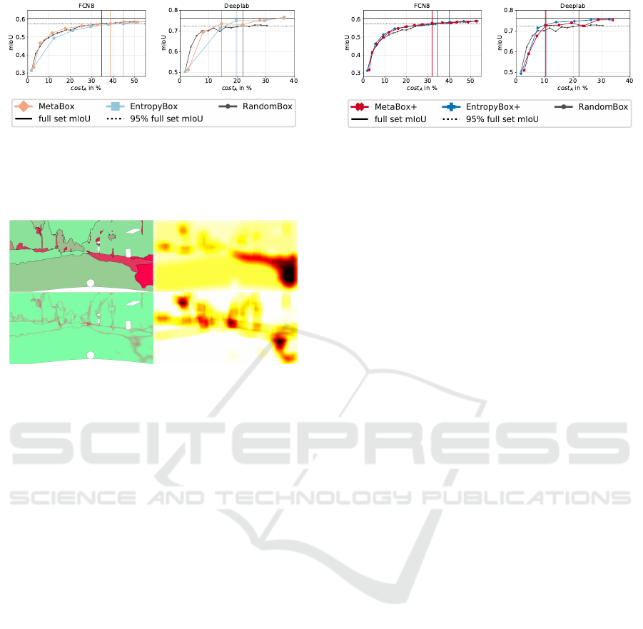
Figure 6: Results of the AL experiments for MetaBox,

EntropyBox and RandomBox. Costs are given in terms

of cost metric cost

. The vertical lines indicate where a

corresponding method achieves 95% full set mIoU. Each

method’s curve represents the mean over 3 runs.

Figure 7: Comparison of query strategies based on MetaSeg

and entropy. In the MetaSeg priority map (top left), low es-

timated IoU values are colored red and high ones green. Ac-

cordingly, in the entropy priority map (bottom left) low con-

ﬁdence is colored red and high conﬁdence is colored green.

The (line-wise) corresponding aggregations are given in the

right hand column. The higher the priority, the darker the

color.

MetaBox and RandomBox. RandomBox produces

relatively small but very consistent costs per AL it-

eration.

Comparison of MetaBox+ and EntropyBox+. In-

corporating the estimated number of clicks improves

both methods MetaBox and EntropyBox, see Fig-

ure 8. For the FCN8 model, EntropyBox+ still pro-

duces more clicks cost

= 40.06% compared to Ran-

domBox. On the other hand, MetaBox+ requires

the lowest costs with cost

= 32.01%. For the

Deeplab model, EntropyBox+ and MetaBox+ pro-

duce almost the same click costs (cost

= 10.25% and

cost

= 10.47%, respectively) for achieving 95% full

set mIoU. By taking the estimated costs into account,

the produced costs per AL iteration are lower for both

methods. Although, in comparison with Entropy-

Box and MetaBox, the methods EntropyBox+ and

MetaBox+ require more AL iterations, both methods

perform better in terms of required clicks to achieve

95% full set mIoU. Due to the incorporation of cost

estimation, both EntropyBox+ and Metabox+ query

regions with lower costs and, as indicated by our re-

sults, with more efﬁciency.

Figure 8: Results of the AL experiments for MetaBox+ and

EntropyBox+. Costs are given in terms of cost metric cost

The vertical lines indicate where a corresponding method

achieves 95% full set mIoU. Each method’s curve repre-

sents the mean over 3 runs.

In general, we observe that the Deeplab model

gains performance quicker than the FCN8 model.

This can be attributed to the fact that the FCN8

framework does not incorporate any data augmenta-

tion while the Deeplab framework uses state-of-the-

art data augmentation and provides a more elaborate

network architecture.

Robustness and Variance. Considering Figure 10,

where the experiments for each CNN model are

shown in one plot, we observe that all methods show

a clear dependence on the CNN model. In our ex-

periments with the FCN8 we also observe that results

show only insigniﬁcant standard deviation over the

different trainings. Hence we did not include a ﬁg-

ure for this ﬁnding and rather focus on discussing the

robustness of the methods with respect to the Deeplab

model.

For the Deeplab model, the methods show a sig-

niﬁcant standard deviation over trainings, especially

the methods MetaBox, MetaBox+ and RandomBox,

see Figure 9. In the ﬁrst AL iterations, RandomBox

rapidly gains performance at low costs. However,

in the range of 95% full set mIoU it rather ﬂuctu-

ates and only slightly gains performance. Beyond the

95% full set mIoU frontier, the methods MetaBox(+)

and EntropyBox(+) still improve at a descent pace.

MetaBox+ and EntropyBox+ nearly achieve the full

set mIoU with approximately the same costs.

Furthermore, when investigating the variation of

results with respect to two different CNN models, we

observe that the discrepancy between the FCN8 and

the Deeplab model is roughly 8 percent points smaller

for MetaBox+ than for EntropyBox+. This shows that

MetaBox+ tends to be more robust with respect to the

choice of CNN model.

Comparison of Cost Metrics. In the evaluation

above, we only consider the cost metric cost

. A com-

parison of cost metrics for both CNN models is given

in Table 1. Note that EntropyBox+* and MetaBox+*

MetaBox+: A New Region based Active Learning Method for Semantic Segmentation using Priority Maps

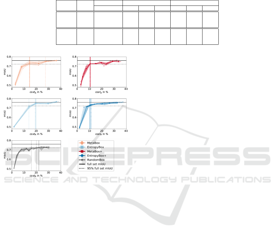
Table 1: Annotation costs in % (row) produced by each method (column) to achieve 95% full set mIoU. Cost metrics cost

(Equation (10)) and cost

(Equation (11)) are based on annotation clicks while cost metric cost

(Equation (12)) indicates

the amount of labeled pixels. The costs with respect to the cost metric of the best performing methods are highlighted. The

strategies EntropyBox+* and MetaBox+* represent a hypothetical “optimum” by knowing the true costs. Each value was

obtained as the mean over 3 runs.

CNN Cost RandomBox EntropyBox MetaBox

model metric + +

∗

+ +

∗

cost

34.54 44.60 40.06 19.82 38.63 32.01 26.61

FCN8 cost

35.76 40.74 37.55 18.87 35.58 30.85 25.74

cost

28.57 10.08 13.45 10.08 12.77 17.81 16.13

cost

22.04 19.61 10.25 10.95 14.48 10.47 16.21

Deeplab cost

22.77 17.92 9.85 10.60 13.56 10.43 15.85

cost

18.49 5.04 5.04 6.72 6.05 7.73 11.09

Figure 9: Results of single AL experiments (consisting of

3 runs each) for each AL method with the Deeplab model.

Costs are given in terms of cost metric cost

. In each plot,

the single runs are given as dotted lines, the mean (over

costs and mIoU) as a solid line. The vertical lines show

where each run achieves 95% full set mIoU.

refer to methods that are equipped with the true costs

from the Cityscapes dataset. We elaborate further

on this aspect in next paragraph. Except for Ran-

domBox, the required costs to achieve 95% full set

mIoU is up to 3 percent points lower when consider-

ing cost

instead of cost

. Considering the proportion

of labeled pixels cost

makes the costs seem signiﬁ-

cantly lower. Noteworthily, for the FCN8 model En-

tropyBox requires only costs of cost

= 10.08% while

RandomBox does require costs of cost

= 28.57%,

which is roughly a factor of 3 higher. Comparing this

with cost

= 44.60% it becomes clear, that these 10%

of the pixels in the dataset constitute to almost half

of the actually required click work. This compari-

son highlights the importance of cost measurement

(deﬁnition of a cost metric) and that the annotation

of image regions requires different human annotation

effort.

Click Estimation. To evaluate our cost estimation

(Section 3.2), we compare it to the provided clicks

in the Cityscapes dataset by considering the latter as

a “perfect” cost estimation. That is, we supply En-

tropyBox and MetaBox with the true costs and term

these methods EntropyBox+* and MetaBox+*. A

comparison of the different click estimations and the

true clicks is given in Table 1. For the FCN8 model,

the experiments show that knowing the true costs in

most cases improves the results: EntropyBox+* pro-

duces costs of cost

= 19.82%. This is the half of the

costs of EntropyBox+. MetaBox+* produces costs of

cost

= 26.61, which is 6 percent points less costs

compared to MetaBox+. For the Deeplab model, us-

ing true rather than estimated costs do not lead to bet-

ter results. However, in terms of cost metric cost

EntropyBox+* produces 1 percent point more costs

then EntropyBox+. MetaBox+* produces even 6 pp.

more costs then MetaBox+. Similarly, we see such

an increase also with respect to the other cost metrics

cost

and cost

5 CONCLUSION

We have introduced a novel AL method MetaBox+,

which is based on the estimated segmentation qual-

ity, combined with a practical cost estimation. We

compared MetaBox(+) to entropy based methods. Us-

ing a combination of entropy and our introduced cost

estimation shows also remarkable results. Our ex-

periments include in-depth studies for two different

CNN models, comparisons of cost metrics, cost / click

estimates, three different query types (Random, En-

tropy, MetaSeg) as well as a study on the robustness.

The new methods MetaBox+ proposed by us lead to

robust reductions in annotation cost, resulting in re-

quiring 10-30% annotation costs for achieving 95%

full set mIoU. All our tests were conducted using a

query function that minimizes the product of two tar-

gets, i.e., minimizing the annotation effort and mini-

ICPRAM 2021 - 10th International Conference on Pattern Recognition Applications and Methods

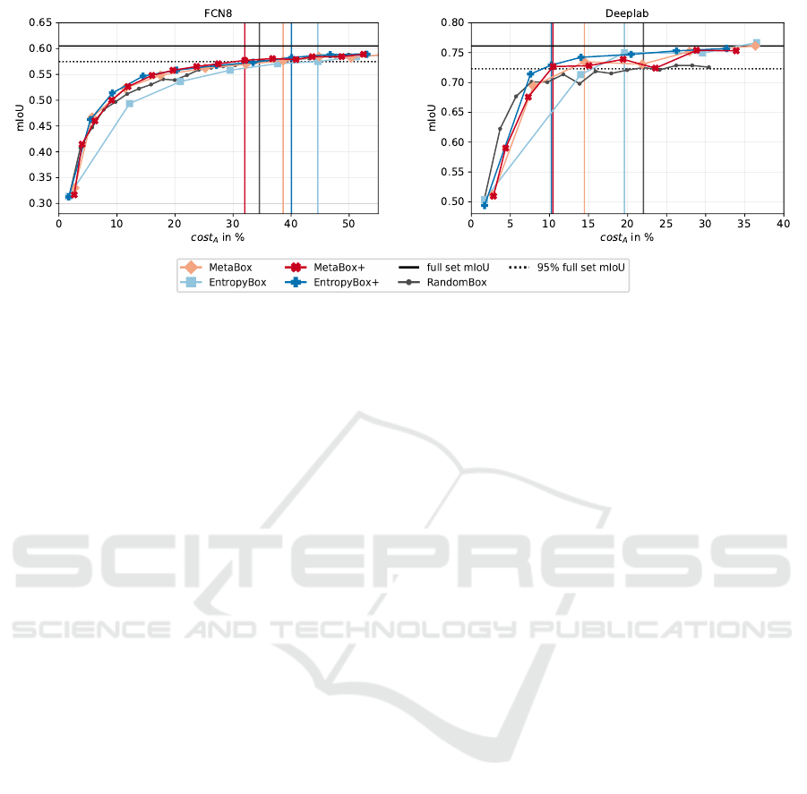
Figure 10: Summary of the results of the AL experiments with the FCN8 model (top) and the Deeplab model (bottom). The

costs are given in cost metric cost

. The vertical lines display where the 95% full set mIoU are achieved. MetaSeg based

method’s have more initial costs due to the data M required for training MetaSeg. Each method’s curve represents the mean

over 3 runs.

mizing the estimated segmentation quality for a given

query region. We leave the question open, whether a

weighted sum of priorities instead of a product Equa-

tion (6) would lead to additional improvements of our

methods. Since each method produces different an-

notation costs per AL iteration, it could be of interest

to vary the number of queried boxes (per AL itera-

tion) or to start each experiment with some Random-

Box iterations. Furthermore, it would be interesting

to also incorporate pseudo labels, i.e., to label regions

of high estimated quality with the predictions of the

CNN model. Semi-supervised approaches remain a

promising direction for further improvements and will

be investigated in the future.

REFERENCES

Beluch, W. H., Genewein, T., Nürnberger, A., and Köhler,

J. M. (2018). The power of ensembles for active learn-

ing in image classiﬁcation. In Proceedings of the IEEE

Conference on Computer Vision and Pattern Recogni-

tion, pages 9368–9377.

Casanova, A., Pinheiro, P. O., Rostamzadeh, N., and Pal,

C. J. (2020). Reinforced active learning for image seg-

mentation. arXiv preprint arXiv:2002.06583.

Chan, R., Rottmann, M., Hüger, F., Schlicht, P., and

Gottschalk, H. (2020). Controlled false negative re-

duction of minority classes in semantic segmentation.

Chen, L.-C., Zhu, Y., Papandreou, G., Schroff, F., and

Adam, H. (2018). Encoder-decoder with atrous sep-

arable convolution for semantic image segmentation.

CoRR, abs/1802.02611.

Chollet, F. (2017). Xception: Deep learning with depth-

wise separable convolutions. 2017 IEEE Conference

on Computer Vision and Pattern Recognition (CVPR),

pages 1800–1807.

Cordts, M., Omran, M., Ramos, S., Rehfeld, T., Enzweiler,

M., Benenson, R., Franke, U., Roth, S., and Schiele,

B. (2016). The cityscapes dataset for semantic urban

scene understanding. In Proc. of the IEEE Conference

on Computer Vision and Pattern Recognition (CVPR).

Dagan, I. and Engelson, S. P. (1995). Committee-based

sampling for training probabilistic classiﬁers. In Ma-

chine Learning Proceedings 1995, pages 150–157. El-

sevier.

Deng, J., Dong, W., Socher, R., Li, L., Kai Li, and Li Fei-

Fei (2009). Imagenet: A large-scale hierarchical im-

age database. In 2009 IEEE Conference on Computer

Vision and Pattern Recognition, pages 248–255.

Douglas, D. H. and Peucker, T. K. (1973). Algorithms for

the reduction of the number of points required to rep-

resent a digitized line or its caricature. Cartographica:

the international journal for geographic information

and geovisualization, 10(2):112–122.

Gal, Y., Islam, R., and Ghahramani, Z. (2017). Deep

bayesian active learning with image data. CoRR,

abs/1703.02910.

Goodfellow, I. J., Shlens, J., and Szegedy, C. (2014). Ex-

plaining and harnessing adversarial examples. arXiv

preprint.

Gorriz, M., Carlier, A., Faure, E., and Giro-i Nieto, X.

(2017). Cost-effective active learning for melanoma

segmentation. arXiv preprint arXiv:1711.09168.

Hahn, L., Roese-Koerner, L., Cremer, P., Zimmermann, U.,

Maoz, O., and Kummert, A. (2019). On the robustness

of active learning. EPiC Series in Computing, 65:152–

162.

Hein, M., Andriushchenko, M., and Bitterwolf, J. (2019).

Why relu networks yield high-conﬁdence predictions

far away from the training data and how to mitigate

the problem. In Proceedings of the IEEE Conference

on Computer Vision and Pattern Recognition, pages

41–50.

Jaccard, P. (1912). The distribution of the ﬂora in the alpine

zone. New Phytologist, 11(2):37–50.

MetaBox+: A New Region based Active Learning Method for Semantic Segmentation using Priority Maps

Jain, S. D. and Grauman, K. (2016). Active image segmen-

tation propagation. In 2016 IEEE Conference on Com-

puter Vision and Pattern Recognition (CVPR), pages

2864–2873.

Kasarla, T., Nagendar, G., Hegde, G. M., Balasubramanian,

V., and Jawahar, C. V. (2019). Region-based active

learning for efﬁcient labeling in semantic segmenta-

tion. In 2019 IEEE Winter Conference on Applications

of Computer Vision (WACV), pages 1109–1117.

Konyushkova, K., Sznitman, R., and Fua, P. (2015). In-

troducing geometry in active learning for image seg-

mentation. In Proceedings of the IEEE International

Conference on Computer Vision, pages 2974–2982.

Long, J., Shelhamer, E., and Darrell, T. (2015). Fully con-

volutional networks for semantic segmentation. In

The IEEE Conference on Computer Vision and Pat-

tern Recognition (CVPR).

Maag, K., Rottmann, M., and Gottschalk, H. (2020). Time-

dynamic estimates of the reliability of deep semantic

segmentation networks. In 2020 IEEE International

Conference on Tools with Artiﬁcial Intelligence (IC-

TAI).

Mackowiak, R., Lenz, P., Ghori, O., Diego, F., Lange, O.,

and Rother, C. (2018). CEREALS - cost-effective

region-based active learning for semantic segmenta-

tion. CoRR, abs/1810.09726.

Mahapatra, D., Bozorgtabar, B., Thiran, J., and Reyes, M.

(2018). Efﬁcient active learning for image classiﬁca-

tion and segmentation using a sample selection and

conditional generative adversarial network. CoRR,

abs/1806.05473.

Mosinska, A., Tarnawski, J., and Fua, P. (2017). Active

learning and proofreading for delineation of curvilin-

ear structures. In International Conference on Med-

ical Image Computing and Computer-Assisted Inter-

vention, pages 165–173. Springer.

Neuhold, G., Ollmann, T., Rota Bulo, S., and Kontschieder,

P. (2017). The mapillary vistas dataset for semantic

understanding of street scenes. In Proceedings of the

IEEE International Conference on Computer Vision,

pages 4990–4999.

Özdemir, F., Peng, Z., Tanner, C., Fürnstahl, P., and Gok-

sel, O. (2018). Active learning for segmentation by

optimizing content information for maximal entropy.

CoRR, abs/1807.06962.

Ramer, U. (1972). An iterative procedure for the polygonal

approximation of plane curves. Computer graphics

and image processing, 1(3):244–256.

Ronneberger, O., Fischer, P., and Brox, T. (2015). U-net:

Convolutional networks for biomedical image seg-

mentation. In International Conference on Medical

image computing and computer-assisted intervention,

pages 234–241. Springer.

Rottmann, M., Colling, P., Hack, T. P., Chan, R., Hüger, F.,

Schlicht, P., and Gottschalk, H. (2020). Prediction er-

ror meta classiﬁcation in semantic segmentation: De-

tection via aggregated dispersion measures of softmax

probabilities. In 2020 International Joint Conference

on Neural Networks (IJCNN), pages 1–9. IEEE.

Rottmann, M., Kahl, K., and Gottschalk, H. (2018).

Deep bayesian active semi-supervised learning. In

2018 17th IEEE International Conference on Machine

Learning and Applications (ICMLA), pages 158–164.

IEEE.

Rottmann, M. and Schubert, M. (2019). Uncertainty mea-

sures and prediction quality rating for the semantic

segmentation of nested multi resolution street scene

images. In Proceedings of the IEEE Conference on

Computer Vision and Pattern Recognition Workshops,

pages 0–0.

Sandler, M., Howard, A. G., Zhu, M., Zhmoginov, A., and

Chen, L.-C. (2018). Inverted residuals and linear bot-

tlenecks: Mobile networks for classiﬁcation, detection

and segmentation. CoRR, abs/1801.04381.

Settles, B. (2009). Active learning literature survey. Com-

puter Sciences Technical Report 1648, University of

Wisconsin–Madison.

Shannon, C. E. (2001). A mathematical theory of communi-

cation, volume 5, pages 3–55. ACM New York, NY,

USA.

Siddiqui, Y., Valentin, J., and Nießner, M. (2019). Viewal:

Active learning with viewpoint entropy for semantic

segmentation. arXiv preprint arXiv:1911.11789.

Sun, C., Shrivastava, A., Singh, S., and Gupta, A. (2017).

Revisiting unreasonable effectiveness of data in deep

learning era. In Proceedings of the IEEE international

conference on computer vision, pages 843–852.

Vezhnevets, A., Buhmann, J. M., and Ferrari, V. (2012).

Active learning for semantic segmentation with ex-

pected change. In 2012 IEEE Conference on Com-

puter Vision and Pattern Recognition, pages 3162–

3169. IEEE.

Wang, J., Sun, K., Cheng, T., Jiang, B., Deng, C., Zhao,

Y., Liu, D., Mu, Y., Tan, M., Wang, X., Liu, W., and

Xiao, B. (2019). Deep high-resolution representation

learning for visual recognition. TPAMI.

Wang, K., Zhang, D., Li, Y., Zhang, R., and Lin, L. (2016).

Cost-effective active learning for deep image classi-

ﬁcation. IEEE Transactions on Circuits and Systems

for Video Technology, 27(12):2591–2600.

Yang, L., Zhang, Y., Chen, J., Zhang, S., and Chen, D. Z.

(2017). Suggestive annotation: A deep active learning

framework for biomedical image segmentation. pages

399–407.

Zhao, H., Shi, J., Qi, X., Wang, X., and Jia, J. (2017).

Pyramid scene parsing network. In Proceedings of

the IEEE conference on computer vision and pattern

recognition, pages 2881–2890.

ICPRAM 2021 - 10th International Conference on Pattern Recognition Applications and Methods