An Investigation Into the Effect of the Learning Rate on Overestimation

Bias of Connectionist Q-learning

Yifei Chen

, Lambert Schomaker

and Marco Wiering

Bernoulli Institute for Mathematics, Computer Science and Artiﬁcial Intelligence, University of Groningen,

9747 AG Groningen, The Netherlands

Keywords:

Reinforcement Learning, Q-learning, Function Approximation, Overestimation Bias.

Abstract:

In Reinforcement learning, Q-learning is the best-known algorithm but it suffers from overestimation bias,

which may lead to poor performance or unstable learning. In this paper, we present a novel analysis of this

problem using various control tasks. For solving these tasks, Q-learning is combined with a multilayer percep-

tron (MLP), experience replay, and a target network. We focus our analysis on the effect of the learning rate

when training the MLP. Furthermore, we examine if decaying the learning rate over time has advantages over

static ones. Experiments have been performed using various maze-solving problems involving deterministic

or stochastic transition functions and 2D or 3D grids and two Open-AI gym control problems. We conducted

the same experiments with Double Q-learning using two MLPs with the same parameter settings, but without

target networks. The results on the maze problems show that for Q-learning combined with the MLP, the

overestimation occurs when higher learning rates are used and not when lower learning rates are used. The

Double Q-learning variant becomes much less stable with higher learning rates and with low learning rates

the overestimation bias may still occur. Overall, decaying learning rates clearly improves the performances of

both Q-learning and Double Q-learning.

1 INTRODUCTION

The core idea of Reinforcement learning (RL) is to

let an agent learn to optimize its behavior by inter-

acting with an environment. The goal of the agent

is to maximize its cumulative obtained reward. To

achieve this goal, the agent learns from trial and error

by observing the effects of different actions in differ-

ent states. This process leads to a temporal sequence:

{ s

, a

, r

, s

, a

, r

, ... } of states s

, actions a

and re-

wards r

, which can be used by the agent to optimize

its action-selection policy (Sutton and Barto, 2018).

The process is stopped when the task is completed

or interrupted in another way, which forms a single

episode (note that continuing tasks also exist, but are

less common in RL). Usually many episodes are re-

quired for learning a near-optimal policy, and there-

fore RL algorithms can take a long time to learn good

policies in complex environments.

A well-known and often used RL algorithm is Q-

learning (Watkins and Dayan, 1992). Q-learning is an

https://orcid.org/0000-0001-8240-0259

https://orcid.org/0000-0003-2351-930X

https://orcid.org/0000-0003-4331-7537

off-policy algorithm and uses bootstrapping for up-

dates. Off-policy learning means the agent uses a tar-

get policy π for updating the value function but uses a

different behavior policy π

for selecting actions (Sut-

ton and Barto, 2018). In this approach, bootstrap-

ping entails the update of the value of the current

state-action pair is based on other action-value esti-

mates, which are usually biased and contain errors.

For solving problems involving large or continuous

state spaces, Q-learning needs to be combined with

function-approximation methods such as neural net-

works, an approach which has already been used suc-

cessfully in the 1990s (Lin, 1993).

The collected data (state, action, target value) dur-

ing training is non-stationary and non-iid. Therefore,

ﬁtting a (non-linear) function on this data may lead

to unstable learning and bad performances. The cur-

rent methodology to deal with this issue is to use

experience replay and a target network (Mnih et al.,

2015), which helps to improve stability, but which

does not solve all problems. One problem that re-

mains is that Q-learning tends to overestimate state-

action values, referred to as the overestimation bias

(Thrun and Schwartz, 1993; Van Hasselt, 2010). Sut-

ton and Barto deﬁned the combination of off-policy

Chen, Y., Schomaker, L. and Wiering, M.

An Investigation Into the Effect of the Learning Rate on Overestimation Bias of Connectionist Q-learning.

DOI: 10.5220/0010227301070118

In Proceedings of the 13th International Conference on Agents and Artiﬁcial Intelligence (ICAART 2021) - Volume 2, pages 107-118

ISBN: 978-989-758-484-8

107

RL, bootstrapping and function approximation as ’the

deadly triad’ (Sutton and Barto, 2018) and several

studies have shown that such algorithms can diverge

(Boyan and Moore, 1994; Wiering, 2004). These

problems sometimes make the application of RL to

solve challenging control tasks very hard.

The problem of overestimation bias in Q-learning

has drawn attention from researchers in RL for many

years. Thrun and Schwartz pointed out that the over-

estimation bias is the major source of failure when

function approximators are combined with Q-learning

(Thrun and Schwartz, 1993). They proved that this

combination could cause a systematic overestimation

of utility values because of the approximation error

and mentioned that this could be resolved by biasing

the function approximator to learn lower predictions.

Later in (Van Hasselt, 2010), van Hasselt showed

that overestimation is quite general in the application

of Q-learning and also occurs when lookup tables are

used to store the state-action value function. To tackle

this problem, van Hasselt proposed an off-policy al-

gorithm called Double Q-learning which does not suf-

fer from overestimation, but which can suffer from

underestimation (Van Hasselt, 2010). Later, van Has-

selt extended the idea of Double Q-learning to us-

ing deep neural networks and constructed an algo-

rithm called Double DQN, which successfully learned

better policies than DQN on different Atari games

(Van Hasselt et al., 2016).

A problem of Double Q-learning is that it does not

solve all problems concerning learning an accurate

state-action value function with function approxima-

tion, because the overestimation problem is replaced

by an underestimation problem. In (D’Eramo et al.,

2016), the authors proposed the Weighted Estimator

to generate more accurate estimations by computing

the weighted averages of the sample means. In (Lu

et al., 2018), the authors identiﬁed another problem

of approximate Q-learning, termed delusional bias.

This delusional bias occurs when value-function up-

dates are generated which are inconsistent with each

other and cannot be jointly realized. To handle this

problem, the authors propose to use information sets,

which are possible function approximator parameter

settings that can justify the updates. These two algo-

rithms are however complex and require much more

computation than regular Q-learning.

Contributions. In this paper we study the over-

estimation bias of Q-learning combined with multi-

layer perceptrons (MLPs) when this QMLP technique

is used to solve different maze-navigation problems

and some other control tasks. QMLP uses experience

replay and a target network and uses the Adam op-

timizer (Kingma and Ba, 2014) to train the MLP on

mini-batches with experiences. We especially exam-

ine the effects of different learning rates on the result-

ing overestimation bias and ﬁnal performance. We

also propose the use of decaying the learning rate in-

stead of using a static learning rate as commonly used

in connectionist RL. Furthermore, we implemented a

Double Q-learning algorithm in which two MLPs are

used to learn two different state-action value functions

similar to the original Double Q-learning algorithm

(Van Hasselt, 2010). For this DQMLP method no tar-

get networks are used.

We created four tasks consisting of 2D or 3D maze

environments and deterministic or stochastic transi-

tion functions. Besides, two classic control prob-

lems from the Open-AI gym environments were used

to further examine the effect of learning rates on

the overestimation bias and performance. The re-

sults showed that when lower learning rates are used

for QMLP, no signiﬁcant overestimation bias occurs.

However, with higher learning rates, the overestima-

tion bias does occur with QMLP. By using a decay-

ing learning rate, the overestimation bias can be sub-

dued and the value estimation can be improved. When

Double Q-learning is combined with MLPs, the re-

sulting DQMLP algorithm sometimes still leads to an

overestimation bias when very low learning rates are

used and becomes less stable when higher learning

rates are used. Again, the value estimation can be im-

proved by using a decaying learning rate. The results

show that higher learning rates lead to worse ﬁnal per-

formances for both algorithms on the maze problems,

although low learning rates lead to lower average per-

formance during a whole simulation, which is caused

by the initial slow learning behavior. Finally, the re-

sults demonstrate that in almost all experiments the

use of a decaying learning rate can considerably im-

prove the ﬁnal and average performances.

Paper Outline. In Section 2, the used RL algo-

rithms and the learning rate decay technique are de-

scribed. Section 3 explains the experimental setup.

In Section 4, the experimental results are presented

and discussed. Section 5 concludes the paper and de-

scribes some directions for future work.

2 REINFORCEMENT LEARNING

In order to formalize most RL problems, the Markov

decision process (MDP) framework can be used

(Howard, 1960). A ﬁnite stationary MDP is a tuple

< S, A, R, P, γ >, where:

• S represents the set of possible states in the envi-

ronment and s

denotes the state at time step t.

ICAART 2021 - 13th International Conference on Agents and Artiﬁcial Intelligence

108

• A is the set of valid actions the agent can take and

denotes the selected action at time step t.

• R(s, a, s

) is the reward function which emits a re-

ward r

t+1

after the agent took action a in state s

and moved to state s

• P(s, a, s

) is the state transition probability func-

tion and gives the probability of transitioning to

state s

if the agent takes action a in state s.

• γ is a discount factor, 0 ≤ γ ≤ 1, and determines

the importance of rewards obtained in the future

compared to immediate rewards.

The goal of an agent is to learn the optimal policy to

obtain the highest possible cumulative discounted re-

ward. In many RL algorithms, the agent uses value

functions that estimate the goodness of states or state-

action pairs. The value of a state, v

(s), denotes the

expected discounted cumulative reward that an agent

obtains when starting from state s and following pol-

icy π:

(s) = E[

∞

∑

k=0

t+k+1

= s] (1)

Where the expectancy operator is used to average over

stochastic transitions and possibly over a stochastic

policy and a stochastic reward function. Similarly, the

state-action values q

(s, a) are deﬁned by:

(s, a) = E[

∞

∑

k=0

t+k+1

= s, a

= a] (2)

An optimal policy π

∗

is associated to the optimal Q-

function q

∗

(s, a), which is the maximum Q-function

over all policies. When the agent correctly estimated

∗

(s, a), it can select optimal actions using π

∗

(s) =

argmax

∗

(s, a).

2.1 Q-learning with a Multilayer

Perceptron

Q-learning (Watkins, 1989; Watkins and Dayan,

1992) is the most often used algorithm for value-

function based RL and can learn the optimal policy

for ﬁnite MDPs even when actions are always taken

completely randomly. This is because of its off-policy

nature and this makes it also suitable for learning

policies from expert demonstrations or for simulta-

neously learning multiple policies that solve different

tasks. Given an experience tuple (s

, a

, r

t+1

, s

t+1

), Q-

learning updates the Q-value Q(s

, a

) according to:

Q(s

, a

) :=Q(s

, a

η(r

t+1

+ γmax

Q(s

t+1

, a

) − Q(s

, a

))

(3)

where η denotes the learning rate. As the agent ex-

plores the effects of different actions in the environ-

ment, the Q-function is continuously updated. When

lookup tables are used to store the Q-function, Q-

learning with a proper learning rate annealing sched-

ule will converge after all actions have been tried an

inﬁnite number of times in all states (Jaakkola et al.,

1994; Tsitsiklis, 1994)

Although the most straightforward way of ap-

plying Q-learning is using a look-up table to store

the Q-values of all state-action pairs, this is infeasi-

ble if the state-action space is very large or continu-

ous. Furthermore, a tabular representation does not

have generalization power, which makes it impossi-

ble for the agent to select an informed action in a

state that has not been visited before. Therefore, us-

ing function approximation is necessary when using

Q-learning for solving complex sequential decision-

making problems. The most often used function

approximation techniques in RL are different kinds

of neural networks. In 1993, Lin combined multi-

layer perceptrons with Q-learning for several chal-

lenging navigation tasks (Lin, 1993), for which he

also proposed the currently popular experience replay

method. Tesauro also used an MLP when training a

backgammon playing program that used self-play and

temporal-difference learning (Tesauro, 1994). The

resulting TD-Gammon program reached a human-

expert level playing performance and was one of the

ﬁrst successes of RL.

More recently, approximating Q-functions by us-

ing convolutional neural networks (CNNs) has been

shown to work very well for solving problems in-

volving huge state spaces. In (Mnih et al., 2013;

Mnih et al., 2015), the authors proposed a novel RL

method, the deep Q-network (DQN), that combines

Q-learning, a CNN, experience replay and a separate

target Q-network. This DQN agent achieved state-of-

the-art performances on 43 Atari games by only us-

ing images containing raw pixel values as input. This

led to the active research ﬁeld of deep reinforcement

learning (DRL), in which deep neural networks are

combined with RL algorithms.

When training neural networks with RL algo-

rithms, an objective or loss function can be speciﬁed.

When Q-learning and a target network are used, the

loss function is:

= E[(r

t+1

+ γmax

Q(s

t+1

, a;θ

−

) − Q(s

, a

;θ))

]

(4)

where θ consists of all trainable parameters of the cur-

rent Q-network, and θ

−

represents the parameters of

the target Q-network which is a backup version of a

previous Q-network. The expectancy operator is used

An Investigation Into the Effect of the Learning Rate on Overestimation Bias of Connectionist Q-learning

109

because training occurs using stochastic sampling of

mini-batches with experiences.

In this paper, we also use this objective function

but instead of a CNN, we use a multilayer percep-

tron and train it with Q-learning. We will call this

approach QMLP and similar to DQN, experience re-

play is used so that the collected experiences can be

used multiple times for training the MLP (Lin, 1993).

Furthermore, a separate target Q-network which is up-

dated periodically is used, which is considered state-

of-the-art practice in DRL to make the method more

stable.

2.2 Double Q-learning with Two

Multilayer Perceptrons

As described in the introduction, Q-learning can suf-

fer from overestimation errors when learning the Q-

function. Furthermore, the combination of off-policy

RL, bootstrapping and function approximation form

the deadly triad (Sutton and Barto, 2018), which can

lead to poor learning performances (Van Hasselt et al.,

2018). There have been different attempts to alleviate

the overestimation bias in Q-learning. In (Van Has-

selt, 2010), van Hasselt proposed an off-policy algo-

rithm, Double Q-learning, which uses a double esti-

mator approach for updating Q-values. Let Q

and

denote the two estimators, then for selecting an

action one of them is selected randomly or the av-

erage action value of both Q-functions can be used.

Then, one Q-function (e.g. Q

) is randomly selected

to be updated using:

, a

) :=Q

, a

η(r

t+1

+ γQ

t+1

, a

) − Q

, a

))

(5)

where a

= argmax

t+1

, a) denotes the optimal

action to take in the next state according to function

. The updating rule for Q

is the same with Q

and

swapped.

Subsequently, Double DQN was developed by

adapting the DQN algorithm with respect to the idea

of Double Q-learning (Van Hasselt et al., 2016). The

update for the Q-network of Double DQN is similar

to the one of DQN, except for the target value of an

update:

DDQN

≡ r

t+1

+ γQ(s

t+1

, argmax

Q(s

t+1

, a;θ

), θ

−

)

(6)

where θ and θ

−

are again the parameters of the Q-

network and the target Q-network. The basic differ-

ence is that the Q-network is used to compute the best

action in the next state instead of letting the target Q-

network determine this best action. It should be noted

that this update is somewhat different from the orig-

inal Double Q-learning algorithm, because only one

network is used for selecting actions and updated on

the experiences.

In our experiments, we developed a DQMLP al-

gorithm that is more similar to the original Double

Q-learning algorithm, which has also been proposed

in (Schilperoort et al., 2018). Our DQMLP algorithm

uses two MLPs to approximate the two estimators of

the Double Q-learning algorithm. For selecting an ac-

tion, the average Q-value of both MLPs is used. For

each training step, one MLP is randomly picked to be

updated, and the other MLP is used to compute the

target value. The loss function for updating the Q

network is:

= E[(r

t+1

+ γQ

t+1

, a

∗

;θ

) − Q

, a

;θ

))

]

(7)

where θ

and θ

represent the parameters of the two

MLPs. The action a

∗

is again determined using net-

work Q

. The update for the Q

network is again the

same with indices swapped.

2.3 Learning Rate Decay

Learning rate decay is a commonly used technique in

deep learning because of its simplicity and effective-

ness (You et al., 2019). In the beginning of training,

a reasonably high learning rate is important to learn

fast, but once a good approximation has been learned,

using a low learning rate helps with ﬁne-tuning the

model. It has been shown that when using stochastic

gradient descent with mini-batches of training data,

annealing the learning rate is necessary for the model

to converge.

In RL, almost all researches use ﬁxed learning

rates and the effect of learning rate decay has hardly

been studied. In (Van Hasselt, 2010), the author used

a linear learning rate and a polynomial learning rate

decay in the experiments, but the effect of using de-

caying learning rates compared to ﬁxed learning rates

was not researched. The relationship between learn-

ing rates and convergence rates in the Q-learning al-

gorithm was explored in (Even-Dar and Mansour,

2003), but the algorithm studied was not combined

with function approximators.

Therefore, besides the impact of learning rates on

the overestimation bias, this paper investigates the ef-

fect of learning rate decay on the value estimation and

performances of approximate RL algorithms.

ICAART 2021 - 13th International Conference on Agents and Artiﬁcial Intelligence

110

3 EXPERIMENTAL SETUP

The experiments were performed in different maze

environments and two Open-AI gym environments:

CartPole-v0 and Acrobot-v1. In this section, we will

ﬁrst describe details of the maze environments. Then

the structure of the MLPs is presented together with

the used hyper-parameters. At the end of this section

we explain how we measured the performances of the

RL algorithms.

3.1 Maze Environments

To investigate when the overestimation occurs in the

QMLP and DQMLP algorithms, an empty 2D maze

and an empty 3D maze were constructed as illustrated

in Figure 1. In each episode of the 2D maze, the agent

starts from the upper left corner (green cell) and has to

navigate to the lower right corner (red cell). The 2D

maze consists of 100 states and four actions: north,

south, west, and east. Similarly, in every episode of

the 3D maze, the agent starts in the green cell and

needs to ﬁnd the red cell. The 3D maze consists of

1000 states and there are six actions: up, down, north,

south, west, and east.

(a) 2D maze (b) 3D maze

Figure 1: Illustration of the 2D and 3D environments. The

following states can be viewed: the starting state (green),

the terminal state (red), and other states (white). Note that

there is a wall around each entire maze, which is not shown

in the ﬁgures.

State Transition Functions. Two types of state

transition functions were created for both mazes: (1)

deterministic transition functions, and (2) stochastic

transition functions. Therefore, four kinds of envi-

ronments were constructed in total: a deterministic

2D maze, a stochastic 2D maze, a deterministic 3D

maze, and a stochastic 3D maze. In the maze with

a deterministic transition function, the agent executes

the selected action deterministically. For the stochas-

tic transition function, the agent has a 20% chance of

randomly moving to one of the neighboring states in-

stead of executing the selected action.

Reward Function. The reward function is kept

the same for all maze environments. The agent gets a

reward of −5 for hitting the borders of the maze and

+20 for reaching the terminal goal state. For every

other step, a punishment of −1 is given to encourage

the agent to ﬁnd the exit using the least number of

steps. The optimal cumulative reward intake in one

episode is +3 for the deterministic 2D maze, and −6

for the deterministic 3D maze. Note that the optimal

Q-value of the best action in the starting state (which

we will also analyse) is different for these environ-

ments due to the discount factor.

3.2 Structure of Multilayer Perceptrons

and Used Hyper-parameters

3.2.1 Maze Environments

In the maze-navigation problems, the MLPs in QMLP

and DQMLP are implemented with the same struc-

ture, but DQMLP uses two MLPs. Each MLP is com-

posed of an input layer, a single hidden layer, and an

output layer.

Input Layer. The input of the MLP uses a con-

tinuous representation of the state of the agent. The

current coordinates of the agent are normalized to val-

ues between 0 and 1. Therefore, the input layer of the

2D maze is composed of 2 nodes, which represent the

row and column index of the agent. The starting state

of the 2D maze is represented as [0.0, 0.0], and the

terminal state is [1.0, 1.0]. Likewise, three inputs are

used for the 3D maze.

Hidden Layer. The number of hidden units is

2048, which was enough to reliably learn to solve

the tasks in preliminary experiments. As activation

function, the hidden units use the rectiﬁed linear unit

(ReLU) function (Glorot et al., 2011).

Output Layer. The outputs of the MLP represent

the Q-values of the actions. Therefore, the number of

output units is the same as the number of actions (4 or

6). A linear activation function is used in the output

layer.

Other Hyper-parameters. The QMLP and

DQMLP agent are both trained using the Adam op-

timizer (Kingma and Ba, 2014). We use the standard

values β

= 0.9 and β

= 0.999 and varied the values

of the learning rate. All other parameters were tuned

using preliminary experiments. The epsilon-greedy

policy is used as exploration strategy. For each sim-

ulation, each agent is trained for 5,000 episodes with

the value of epsilon decaying linearly from 1.0 to 0.0

in the ﬁrst 4,000 episodes and staying at 0.0 in the last

1,000 episodes. The maximum number of steps in one

episode is set to 2,000. The discount factor is 0.95. In

every updating step, a batch size of 128 experiences

is sampled from the experience replay buffer for the

agent to learn from. The capacity of the experience

replay memory is 20,000. The best results were ob-

An Investigation Into the Effect of the Learning Rate on Overestimation Bias of Connectionist Q-learning

111

tained by copying the current Q-network to the target

network after each step and therefore this means that

essentially no target network is used for QMLP.

3.2.2 Open-AI Gym Environments

For solving the Open-AI gym problems, the hyper-

parameters were slightly re-tuned. Both QMLP and

DQMLP agents are trained for 500 episodes. The

epsilon value decreases linearly from 1.0 to 0.0 in

the ﬁrst 400 episodes and stays 0.0 for the remain-

ing episodes. For both agents, the MLP used two

hidden layers, the ﬁrst with 48 and the second with

96 hidden units. The capacity of the memory buffer

is 1,000,000. The batch size is 512 for both algo-

rithms. The target network of QMLP is updated ev-

ery 64 steps. The other hyper-parameters are kept the

same as for the maze-solving agents.

3.3 Performance Measures

In the results, we report three different performance

measures. First, the cumulative reward intake dur-

ing the last episode is recorded for each simulation.

Second, the average cumulative reward per episode

during an entire simulation is computed. Third, to an-

alyze possible overestimation or underestimation er-

rors, we record the estimated maximal Q-value of the

starting state. Because the Q-values of the initial state

can change during the entire episode due to the use

of experience replay after each time step, the average

initial state value is computed for each episode. Equa-

tion (8) shows the computation of the initial state-

value estimate per episode.

start

∑

t=1

max

Q(S

start

, a;θ) (8)

Where T denotes the number of steps in an episode

(T ≤ 2000 for maze-navigation problems), and θ rep-

resents the weight values of the Q-network. For

DQMLP, two Q-functions are learned and we selected

the highest Q-value for the initial state from both Q-

functions to compute the initial state value. The true

maximum state-action value of the starting state in

each maze environment was calculated by using dy-

namic programming (Bellman, 1957).

4 EXPERIMENTAL RESULTS

The results are obtained by running 10 simulations

with different random seeds. For each episode, the

initial state value estimate V

start

and the cumulative re-

ward sum R are recorded. In each ﬁgure for the value

estimates in the following subsections, the straight

red line represents the true optimal value of the start-

ing state in each corresponding environment. Each

curve shows the average result of the 10 runs, and the

shaded regions show the standard deviation. Some

parts of the ﬁgures were zoomed in for clarity.

In 2D mazes, The learning curves of using the

learning rates: 5e − 3, 1e − 3, 1e − 4, 1e − 5, 1e − 6,

and a decaying learning rate are plotted. While in 3D

mazes and the Open-AI gym control environments,

the learning rates 1e − 3, 1e − 4, 1e − 5, 1e − 6, and

a decaying learning rate are used. Speciﬁcally, the

decaying learning rate is set as 10

with x linearly an-

nealing from -3 to -6 over all the episodes. The setting

of the decaying learning rate is kept the same in the

following experiments.

4.1 Results on Maze Environments

4.1.1 Deterministic 2D Maze

The ﬁrst row in Figure 2 shows the estimated initial

state value and the cumulative reward per episode of

the QMLP agent in the deterministic 2D maze. We

can see from Figure 2a that overestimation occurred

with the learning rates 5e − 3 and 1e − 3. The cor-

responding cumulative reward curves became unsta-

ble after around 4300 episodes as shown in Figure 2b.

The agent performed best with the decaying learning

rate: the corresponding cumulative rewards smoothly

converged and the average reward intake was highest.

When we examine the results for DQMLP in Fig-

ure 2c, we can observe that the initial state-value es-

timate curves become unstable for the learning rates

5e − 3 and 1e − 3, and their corresponding cumula-

tive rewards were also deteriorating as shown in Fig-

ure 2d. The agent had a stable learning behavior and

achieved the optimal cumulative rewards of +3 with a

learning rate of 1e−4, 1e −5, 1e −6 and the decaying

learning rate. When we zoom in, we can observe that

DQMLP with a learning rate of 1e − 6 surprisingly

starts to overestimate the initial state value in the end.

Table 1 shows the results of both algorithms in the

last episode for the initial state value estimate V and

the cumulative reward R, where σ represents the stan-

dard deviation. The table also shows the average cu-

mulative reward

R over all episodes. The table clearly

shows the overestimation errors for QMLP when high

learning rates are used. The table also shows that

DQMLP always obtains the highest cumulative re-

ward in the last episode, but QMLP learns faster and

obtains higher average rewards over all episodes. De-

caying the learning rate leads to the best performances

for both algorithms: the value function is accurate and

ICAART 2021 - 13th International Conference on Agents and Artiﬁcial Intelligence

112

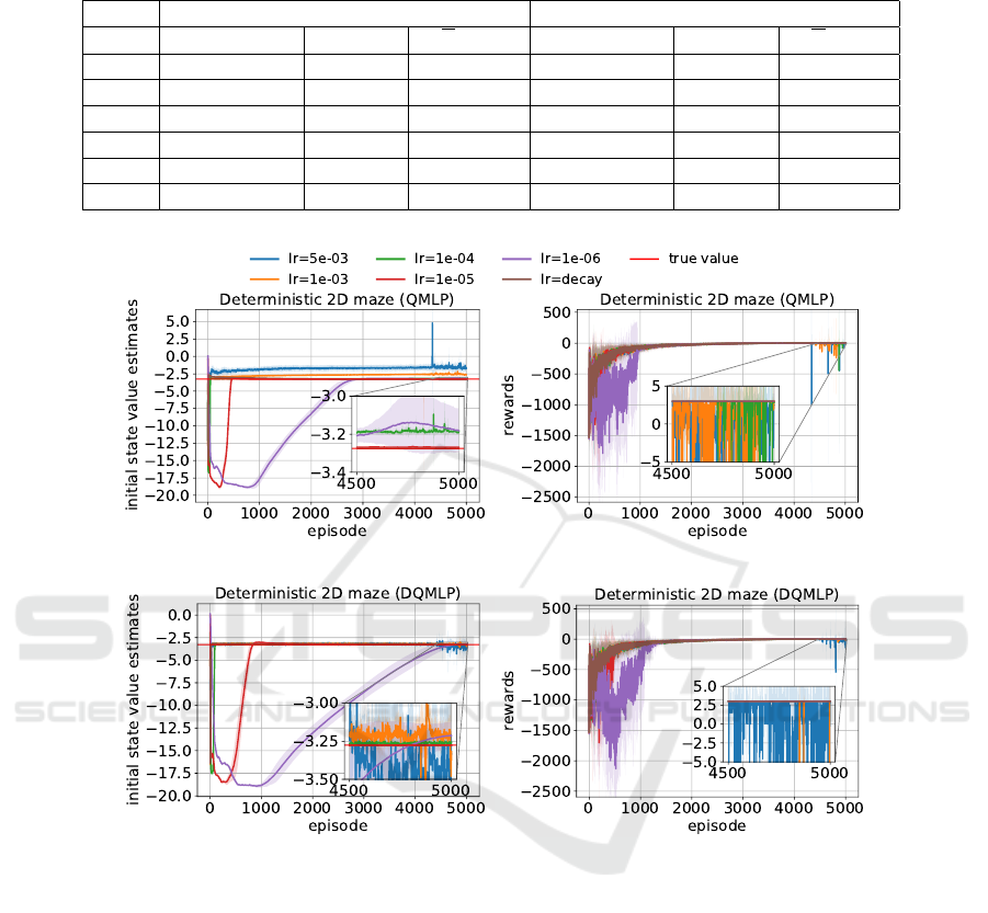
Table 1: Results of QMLP and DQMLP in a deterministic 2D maze. The true value for the initial state is -3.28 and the optimal

cumulative reward is +3.0.

QMLP DQMLP

l.r. V ± σ R ± σ R ± σ V ± σ R ± σ R ± σ

5e-3 −1.71 ± 0.37 2.5 ± 1.5 −57 ± 2 −3.33 ± 0.60 3.0 ± 0.0 −60 ± 1

1e-3 −2.63 ± 0.13 3.0 ± 0.0 −56 ± 1 −3.32 ± 0.33 3.0 ± 0.0 −59 ± 1

1e-4 −3.19 ± 0.01 2.8 ± 0.6 −56 ± 0 −3.26 ± 0.01 3.0 ± 0.0 −59 ± 1

1e-5 −3.27 ± 0.00 3.0 ± 0.0 −67 ± 2 −3.28 ± 0.00 3.0 ± 0.0 −78 ± 8

1e-6 −3.18 ± 0.12 3.0 ± 0.0 −151 ± 20 −3.21 ± 0.09 3.0 ± 0.0 −195 ± 26

decay −3.28 ± 0.00 3.0 ± 0.0 −55 ± 1 −3.28 ± 0.00 3.0 ± 0.0 −58 ± 1

(a) QMLP: V

start

(b) QMLP: Reward Sum

start

(d) DQMLP: Reward Sum

Figure 2: Performances of the QMLP agent and the DQMLP agent in a deterministic 2D maze with different learning rates.

Each curve shows the average results of 10 runs. The shaded regions show the standard deviation.

the average reward intake over all episodes is highest.

At the end of training this method is also much more

stable than using static higher learning rates.

4.1.2 Deterministic 3D Maze

The results for the QMLP and DQMLP agent in a de-

terministic 3D maze are shown in Table 2. The table

shows clear overestimation errors for QMLP when the

learning rate is 1e − 3. For DQMLP, signiﬁcant over-

estimation errors occur for the lowest learning rate.

The use of a decaying learning rate is again very use-

ful for both algorithms: the accuracy of the value

function, the ﬁnal performance and the average per-

formance are all excellent using the decay function.

We also noticed that using higher learning rates again

led to instabilities in the learning process.

4.1.3 Stochastic 2D Maze

The ﬁrst row of Figure 3 shows the training results of

the QMLP agent in a stochastic 2D maze. As reported

in Figure 3a, with a learning rate of 5e − 3, 1e − 3

and 1e − 4, the agent signiﬁcantly overestimated the

value of the starting state. Large standard deviations

(shaded areas) can also be seen in the curve with a

learning rate of 5e − 3. Figure 3b shows that QMLP

with a learning rate of 1e − 5, 1e − 6 and the decaying

An Investigation Into the Effect of the Learning Rate on Overestimation Bias of Connectionist Q-learning

113

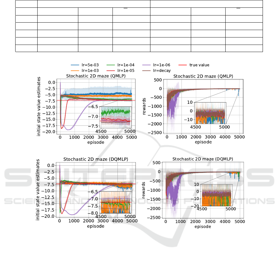
Table 2: Results of QMLP and DQMLP in a deterministic 3D maze. The true value for the initial state is -9.46 and the optimal

cumulative reward is -6.0.

QMLP DQMLP

l.r. V ± σ R ± σ R ± σ V ± σ R ± σ R ± σ

1e-3 −7.39 ± 1.52 −6.4 ± 0.8 −195 ± 80 −9.95 ± 1.73 −6.2 ± 0.6 −171 ± 2

1e-4 −9.18 ± 0.04 −6.0 ± 0.0 −156 ±2 −9.40 ± 0.10 −6.0 ± 0.0 −163 ± 2

1e-5 −9.45 ± 0.00 −6.0 ± 0.0 −170 ± 11 −9.47 ± 0.01 −6.0 ± 0.0 −254 ± 21

1e-6 −9.35 ± 0.07 −6.0 ± 0.0 −734 ± 117 −8.67 ± 0.57 −6.0 ± 0.0 −1151 ± 41

decay −9.44 ± 0.04 −6.0 ± 0.0 −157 ± 4 −9.47 ± 0.01 −6.0 ± 0.0 −117 ± 2

(a) QMLP: V

start

(b) QMLP: Reward Sum

start

(d) DQMLP: Reward Sum

Figure 3: Performances of the QMLP and DQMLP agent in a stochastic 2D maze. Each curve shows the average results of

10 runs.

learning rate performed the most stable.

As can be seen from Figure 3c, for DQMLP with

a learning rate of 5e −3, 1e −3 or 1e− 4, the value es-

timate became unstable. Their corresponding cumu-

lative reward curves also became oscillating as shown

in Figure 3d. The agent ﬁnally performed best with

a learning rate of 1e − 5, 1e − 6 or a decaying learn-

ing rate. In the end, DQMLP again overestimates the

initial state value with a learning rate of 1e − 6.

The results on the stochastic 2D maze are also

shown in Table 3. The table shows large overestima-

tion errors for QMLP with the highest learning rates.

DQMLP signiﬁcantly underestimates the initial state

value when a learning rate of 1e − 3 is used and over-

estimates the value with a learning rate of 1e− 6. Due

to the stochasticity of the environment, the cumulative

rewards of the last episode have large standard devi-

ations, but we can observe that the highest learning

rate leads to worse performances for both algorithms.

Decaying the learning rate was again beneﬁcial for

QMLP, but DQMLP had a few bad episodes with it at

the end, which explains the high standard deviation.

4.1.4 Stochastic 3D Maze

The results for the QMLP and DQMLP agent in the

stochastic 3D maze are shown in Table 4. The ta-

ble shows signiﬁcant overestimation errors for QMLP

with the highest used learning rate. Furthermore, with

all learning rates DQMLP learns to underestimate the

ICAART 2021 - 13th International Conference on Agents and Artiﬁcial Intelligence

114

Table 3: Results of QMLP and DQMLP in a stochastic 2D maze. The true value for the initial state is -7.23 and the optimal

cumulative reward is -2.4.

QMLP DQMLP

l.r. V ± σ R ± σ R ± σ V ± σ R ± σ R ± σ

5e-3 −4.60 ± 2.65 −5.7 ± 5.2 −76 ±3 −8.12 ± 1.02 −6.8 ± 6.7 −80 ± 3

1e-3 −5.54 ± 0.46 −2.2 ± 4.4 −74 ±1 −7.34 ± 0.42 −6.1 ± 6.2 −76 ± 1

1e-4 −6.76 ± 0.29 −3.6 ± 5.9 −77 ±2 −7.42 ± 0.35 −2.1 ± 5.0 −78 ± 2

1e-5 −7.24 ± 0.17 −2.8 ± 3.9 −74 ±1 −7.23 ± 0.20 −3.4 ± 6.0 −76 ± 2

1e-6 −7.28 ± 0.19 −2.3 ± 3.9 −142 ± 27 −6.98 ± 0.19 −2.2 ± 5.3 −200 ± 15

decay −7.28 ± 0.15 −2.1 ± 4.3 −74 ± 1 −7.71 ± 0.33 −5.3 ± 7.4 −76 ± 1

Table 4: Results of QMLP and DQMLP in a stochastic 3D maze. The true value for the initial state is -13.36 and the optimal

cumulative reward is -14.2.

QMLP DQMLP

l.r. V ± σ R ± σ R ± σ V ± σ R ± σ R ± σ

1e-3 −9.56 ± 0.48 −20.2 ± 10.5 −208 ± 2 −14.93 ± 1.18 −39.0 ± 60.8 −222 ± 3

1e-4 −13.27 ± 0.26 −18.1 ± 7.0 −381 ± 63 −14.78 ± 0.29 −18.9 ± 8.9 −317 ± 32

1e-5 −15.18 ± 0.83 −20.1 ± 7.5 −276 ± 49 −15.20 ± 0.35 −19.0 ± 8.4 −329 ± 12

1e-6 −15.45 ± 0.96 −20.1 ± 6.0 −1110 ± 280 −18.16 ± 3.44 −119 ± 116.2 −928 ± 77

decay −14.89 ± 0.49 −17.1 ± 5.6 −209 ± 3 −15.54 ± 0.34 −19.9 ± 6.6 −225 ± 2

value of the initial state.

For QMLP, the value estimate converged when the

learning rate is 1e − 4. With a learning rate of 1e − 6,

the standard deviation of the value estimate curve be-

came large and it seems the algorithm needs more

episodes to converge. The best used learning rate is

the decaying learning rate, which leads to the best ﬁ-

nal cumulative reward and average reward.

For DQMLP, the agent with a decaying learning

rate performed best: it obtained the highest average

reward and the ﬁnal cumulative reward was among

the best. When the learning rate is 1e − 6, the agent

performed the worst. Also with DQMLP, the algo-

rithm needs more episodes to converge with this low

learning rate.

4.2 Results on Open-AI Gym Problems

As we have seen from the previous results, the agent

using a decaying learning rate performed the best in

the experiments with the empty maze environments.

To further examine the effect of annealing the learning

rate, we additionally conducted experiments on two

classic control problems provided by Open-AI Gym:

CartPole-v0 and Acrobot-v1.

4.2.1 Results on CartPole-V0

The CartPole-v0 problem requires the agent to push a

cart left or right in order to keep a pole standing on the

cart from falling, while keeping the cart on the track.

There are four inputs: cart position and velocity and

the pole’s angle and the angular velocity. There are

two actions: push the cart to the left or right. It is a

well-known control problem that has been researched

extensively.

Optimal Values. In the CartPole-v0 environment,

the agent gets a reward of +1 for every step that the

pole does not fall over. The episode terminates when

either the pole angle or the cart position is out of range

or the episode length reaches the maximum of 200

steps. The value of the discount factor γ is 0.95. This

means that the maximal cumulative reward is 200 and

the optimal Q-value is

∑

199

t=0

1 ∗ γ

≈ 19.999.

Results. The learning curves are presented in Fig-

ure 4. For this problem, low learning rates do not

lead to good performances. The best performance

for QMLP and DQMLP is obtained with the decay-

ing learning rate. Table 5 shows some more details

about the value estimation and performances of both

algorithms in CartPole. It shows that DQMLP with

the decaying learning rate is always able to obtain

the optimal performance. Note that ﬁgure 4(c) shows

that a large overestimation bias occurs in DQMLP,

which was also shown in a similar algorithm (Fuji-

moto et al., 2018). Double DQN, which is a vari-

ant of DQMLP, can also overestimate the true value

(Van Hasselt et al., 2016) in some cases.

4.2.2 Results on Acrobot-V1

The goal of the Acrobot-v1 problem is to swing

up a robot consisting of 2 links and 2 joints. The

problem consists of 6 inputs and there are 3 actions

An Investigation Into the Effect of the Learning Rate on Overestimation Bias of Connectionist Q-learning

115

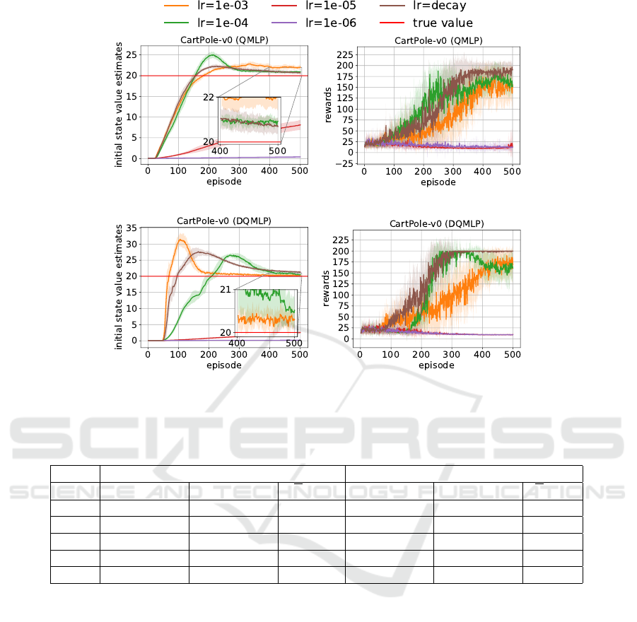
(a) QMLP: V

start

(b) QMLP: Reward Sum

start

(d) DQMLP: Reward Sum

Figure 4: Performances of the QMLP and DQMLP agent in CartPole-v0. Each curve shows the average results of 10 runs.

Table 5: Results of QMLP and DQMLP in the CartPole-v0 environment. The true value for the initial state of CartPole-v0 is

19.999 and the optimal cumulative reward is 200.

QMLP (CartPole-v0) DQMLP (CartPole-v0)

l.r. V ± σ R ± σ R ± σ V ± σ R ± σ R ± σ

1e-3 22.06 ± 0.65 155.6 ± 43.8 81 ± 5 20.30 ± 0.19 168.7 ± 40.2 88 ± 7

1e-4 20.93 ± 0.18 151.9 ± 29.6 107 ± 7 20.52 ± 0.40 160.9 ± 32.5 110 ± 4

1e-5 8.12 ± 1.23 13.3 ± 8.6 14 ± 1 2.55 ± 0.30 9.8 ± 0.6 14 ±1

1e-6 0.38 ± 0.21 11.9 ± 6.5 17 ± 7 0.15 ± 0.04 9.3 ± 0.6 14 ±1

decay 20.69 ± 0.35 190.3 ± 18.7 110 ± 10 21.26 ± 0.32 200.0 ± 0.0 130 ± 3

left/right/do-nothing which is the torque applied on

the second joint.

Optimal Values. For the Acrobot-v1 environ-

ment, there is not a clear optimal cumulative reward,

so we approximate it. The agent gets a punishment of

−1 for every time step until it reaches the goal. The

problem is considered solved when the agent gets an

average reward of -100.0 over 100 consecutive trials.

The value of the discount factor γ is 0.95, and there-

fore we calculated the approximate optimal Q-value

as follows:

∑

t=0

−1 ∗ γ

≈ −19.882.

Results. Table 6 shows the value estimation and

performances of both algorithms in the Acrobot envi-

ronment. The learning curves are presented in Figure

5. As is shown in the results, QMLP with a decaying

learning rate performed very well. The ﬁnal perfor-

mance is very good and the average performance is

the best of all tested learning rates.

For the DQMLP agent, a learning rate of 1e − 4

works the best in the Acrobot environment. The de-

caying learning rate combined with DQMLP leads

again to several bad runs.

4.3 Discussion

From the results, we observe that overestimation er-

rors occur in QMLP with a high learning rate in the

maze problems, no matter whether there is noise in

the environment. For example, in both the determin-

istic 2D maze (ﬁrst row of Figure 2) and the stochas-

tic 2D maze (ﬁrst row of Figure 3), obvious overesti-

mation errors appeared for high learning rates. This

means that noise in the environment is not the pri-

mary cause of overestimation in our cases. There-

ICAART 2021 - 13th International Conference on Agents and Artiﬁcial Intelligence

116

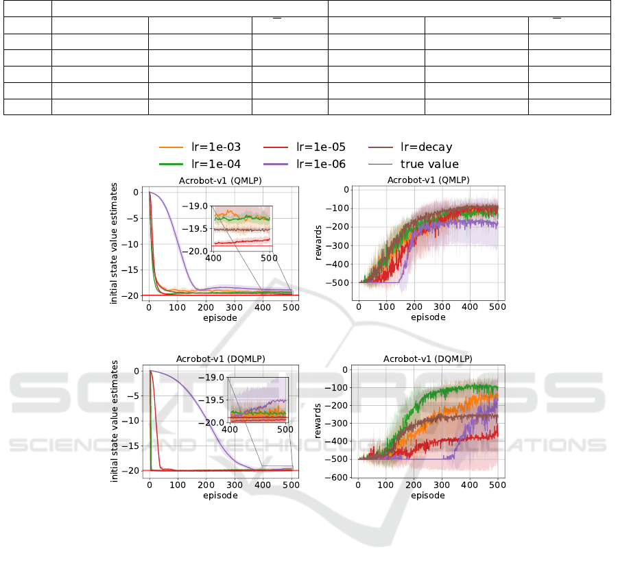
Table 6: Results of QMLP and DQMLP in the Acrobot-v1 environment. The approximate true value for the initial state of

Acrobot-v1 is -19.882 and the approximate optimal cumulative reward is -100.

QMLP (Acrobot-v1) DQMLP (Acrobot-v1)

l.r. V ± σ R ± σ R ± σ V ± σ R ± σ R ± σ

1e-3 −19.26 ± 0.34 −104.0 ± 17.9 −236 ± 13 −19.87 ± 0.21 −148.4 ± 26.7 −315 ± 73

1e-4 −19.27 ± 0.10 −129.7 ± 40.8 −228 ± 27 −19.80 ± 0.13 −98.0 ± 16.9 −237 ± 28

1e-5 −19.72 ± 0.09 −93.7 ± 16.6 −255 ± 47 −19.93 ± 0.13 −373.4 ± 176.2 −428 ± 102

1e-6 −18.85 ± 0.46 −181.6 ± 123.1 −295 ± 73 −19.52 ± 0.53 −171.8 ± 126.5 −433 ± 30

decay −19.51 ± 0.06 −98.7 ± 34.5 −207 ± 10 −19.88 ± 0.21 −265.7 ± 194.0 −335 ± 132

(a) QMLP: V

start

(b) QMLP: Reward sum

start

(d) DQMLP: Reward sum

Figure 5: Performances of the QMLP and DQMLP agent in Acrobot-v1. Each curve shows the average results of 10 runs.

fore, we conclude that the problem occurs because of

function approximation errors that lead to estimating

inconsistent subsequent state-action values. For the

problems we studied, using a decaying learning rate

worked well to handle overestimation errors. Lower

learning rates can also lead to good performances, but

for some problems they lead to very slow learning.

When examining the used combination of Dou-

ble Q-learning with MLPs, where two MLPs learn

two different Q-functions, we observed that with low

learning rates, the DQMLP algorithm can suffer from

the overestimation bias. This could be caused when

both Q-function approximations become almost iden-

tical, in which case the algorithm is similar to QMLP.

In the DQMLP algorithm, actions were selected by

combining both Q-functions. It might be possible that

overestimation bias is less likely when one Q-function

is randomly selected to select an action. The DQMLP

algorithm did not use target networks and although for

the deterministic environments, this did not seem to

be a problem, the learning behavior in the stochastic

environments was less stable than the one of QMLP.

5 CONCLUSION

This paper described a novel analysis of when and

why the overestimation bias may occur when Q-

learning is combined with multilayer perceptrons.

The focus of our study was on the effect of the learn-

ing rate, and we proposed the use of decaying learning

rates in reinforcement learning. The results on four

An Investigation Into the Effect of the Learning Rate on Overestimation Bias of Connectionist Q-learning

117

different grid-worlds demonstrated that the overesti-

mation problem always occurred when higher learn-

ing rates were used and not with lower learning rates

or decaying learning rates.

We also analyzed the performance of Double Q-

learning with multilayer perceptrons under the same

conditions. This algorithm in general suffers from

more underestimation when higher learning rates are

used and surprisingly can also suffer from the overes-

timation bias when very low learning rates are used.

We also examined the performances of both algo-

rithms on two Open-AI gym control problems. The

results obtained on all six environments suggest that

in general the best performances are achieved by us-

ing the decaying learning rates.

Our future work includes studying the connection

between the learning rate and overestimation bias for

more complex environments. We also want to per-

form more research on different methods for anneal-

ing the learning rate over time.

ACKNOWLEDGEMENTS

We would like to thank the Center for Information

Technology of the University of Groningen for their

support and for providing access to the Peregrine high

performance computing cluster. Yifei Chen acknowl-

edges the China Scholarship Council (Grant number:

201806320353) for ﬁnancial support.

REFERENCES

Bellman, R. (1957). Dynamic programming. Princeton Uni-

versity Press, Princeton, NJ, USA, 1 edition.

Boyan, J. A. and Moore, A. W. (1994). Generalization

in reinforcement learning: Safely approximating the

value function. In Proceedings of the 7th Interna-

tional Conference on Neural Information Processing

Systems, pages 369–376. MIT Press.

D’Eramo, C., Restelli, M., and Nuara, A. (2016). Esti-

mating maximum expected value through gaussian ap-

proximation. In International Conference on Machine

Learning, pages 1032–1040. PMLR.

Even-Dar, E. and Mansour, Y. (2003). Learning rates for

q-learning. Journal of machine learning Research,

5(Dec):1–25.

Fujimoto, S., Van Hoof, H., and Meger, D. (2018). Ad-

dressing function approximation error in actor-critic

methods. arXiv preprint arXiv:1802.09477.

Glorot, X., Bordes, A., and Bengio, Y. (2011). Deep sparse

rectiﬁer neural networks. In Proceedings of the four-

teenth international conference on artiﬁcial intelli-

gence and statistics, pages 315–323.

Howard, R. A. (1960). Dynamic Programming and Markov

Processes. MIT Press.

Jaakkola, T., Jordan, M. I., and Singh, S. P. (1994). Con-

vergence of stochastic iterative dynamic programming

algorithms. In Advances in neural information pro-

cessing systems, pages 703–710.

Kingma, D. P. and Ba, J. (2014). Adam: A

method for stochastic optimization. arXiv preprint

arXiv:1412.6980.

Lin, L.-J. (1993). Reinforcement learning for robots using

neural networks. PhD thesis, Carnegie Mellon Uni-

versity, USA.

Lu, T., Schuurmans, D., and Boutilier, C. (2018). Non-

delusional q-learning and value-iteration. In Ad-

vances in Neural Information Processing Systems,

volume 31, pages 9949–9959. Curran Associates, Inc.

Mnih, V., Kavukcuoglu, K., Silver, D., Graves, A.,

Antonoglou, I., Wierstra, D., and Riedmiller, M.

(2013). Playing atari with deep reinforcement learn-

ing. arXiv preprint arXiv:1312.5602.

Mnih, V., Kavukcuoglu, K., Silver, D., Rusu, A. A., Ve-

ness, J., Bellemare, M. G., Graves, A., Riedmiller, M.,

Fidjeland, A. K., Ostrovski, G., et al. (2015). Human-

level control through deep reinforcement learning. na-

ture, 518(7540):529–533.

Schilperoort, J., Mak, I., Drugan, M. M., and Wiering,

M. A. (2018). Learning to play pac-xon with q-

learning and two double q-learning variants. In 2018

IEEE Symposium Series on Computational Intelli-

gence (SSCI), pages 1151–1158. IEEE.

Sutton, R. S. and Barto, A. G. (2018). Reinforcement learn-

ing: An introduction. MIT press, 2nd edition.

Tesauro, G. (1994). Td-gammon, a self-teaching backgam-

mon program, achieves master-level play. Neural

computation, 6(2):215–219.

Thrun, S. and Schwartz, A. (1993). Issues in using function

approximation for reinforcement learning. In Pro-

ceedings of the 1993 Connectionist Models Summer

School. Erlbaum Associates.

Tsitsiklis, J. N. (1994). Asynchronous stochastic approxi-

mation and q-learning. Machine learning, 16(3):185–

202.

Van Hasselt, H. (2010). Double q-learning. In Advances in

Neural Information Processing Systems, pages 2613–

2621. Curran Associates, Inc.

Van Hasselt, H., Doron, Y., Strub, F., Hessel, M., Son-

nerat, N., and Modayil, J. (2018). Deep reinforce-

ment learning and the deadly triad. arXiv preprint

arXiv:1812.02648.

Van Hasselt, H., Guez, A., and Silver, D. (2016). Deep re-

inforcement learning with double q-learning. In Thir-

tieth AAAI conference on artiﬁcial intelligence. AAAI

Press.

Watkins, C. J. C. H. (1989). Learning from delayed rewards.

PhD thesis, King’s College, Cambridge, UK.

Watkins, C. J. C. H. and Dayan, P. (1992). Q-learning. Ma-

chine learning, 8(3-4):279–292.

Wiering, M. A. (2004). Convergence and divergence in

standard and averaging reinforcement learning. In

Proceedings of the 15th European Conference on Ma-

chine Learning, pages 477–488. Springer-Verlag.

You, K., Long, M., Wang, J., and Jordan, M. I. (2019).

How does learning rate decay help modern neural net-

works? arXiv preprint arXiv:1908.01878.

ICAART 2021 - 13th International Conference on Agents and Artiﬁcial Intelligence

118