Learning to Correct Reconstructions from Multiple Views

tefan S

aftescu and Paul Newman

Oxford Robotics Institute, University of Oxford, U.K.

Keywords:

Deep Learning, Multi-view Fusion, Reconstruction, Mesh Correction.

Abstract:

This paper is about reducing the cost of building good large-scale reconstructions post-hoc. This is an important

consideration for survey vehicles which are equipped with sensors which offer mixed ﬁdelity or are restricted by

road rules to high-speed traversals. We render 2D views of an existing, lower-quality, reconstruction and train

a convolutional neural network (

CNN

) that reﬁnes inverse-depth to match to a higher-quality reconstruction.

Since the views that we correct are rendered from the same reconstruction, they share the same geometry, so

overlapping views complement each other. We impose a loss during training which guides predictions on

neighbouring views to have the same geometry and has been shown to improve performance. In contrast to

previous work, which corrects each view independently, we also make predictions on sets of neighbouring

views jointly. This is achieved by warping feature maps between views and thus bypassing memory-intensive

computation. We make the observation that features in the feature maps are viewpoint-dependent, and propose

a method for transforming features with dynamic ﬁlters generated by a multi-layer perceptron from the relative

poses between views. In our experiments we show that this last step is necessary for successfully fusing feature

maps between views.

1 INTRODUCTION

Building good dense reconstructions is essential in

many robotics tasks, such as surveying, localisation,

or planning. Despite numerous advancements in both

hardware and techniques, large-scale reconstructions

remain costly to build.

We approach this issue by trying to reduce the

data acquisition cost either through the use of cheaper

sensors, or by collecting less data. To make up for the

cheaper but lower quality data, we have to turn to prior

information from the operational environment (e.g.

roads and buildings are ﬂat, cars and trees have speciﬁc

shapes, etc). To learn these priors, we train a

CNN

over 2D views of reconstructions, and predict reﬁned

inverse-depth maps that can be fused back into an

improved reconstruction. We take this detour through

two dimensions in order to avoid the high memory

requirements that a volumetric approach over large-

scale reconstructions would impose.

While operating in 2D, neighbouring views are

related by the underlying geometry. Previous work

aftescu and Newman, 2020) has leveraged this re-

lation during training, where a geometric consistency

loss is imposed between neighbouring views that pe-

nalises mismatched geometry. Here, we improve the

adeptness of this approach by showing how neigh-

bouring views can be used together when predicting

reﬁned depth, and to that end introduce a method for

aggregating feature maps in the CNN.

To fuse feature maps from multiple views, we

could either “un-project” them into a common volume

or “collect” them into a common target view through

reprojection, as proposed by (Donne and Geiger, 2019).

As un-projecting into re-introduces the limitation we

wished to avoid, we take the latter approach.

Directly aggregating feature maps between views

– either in a volume or in a common target view – im-

plies features are somewhat independent of viewpoint.

To lift this restriction, this paper proposes a method

for transforming features between views, enabling us

to more easily aggregate feature maps from arbitrary

viewpoints. Concretely, we use the relative pose be-

tween views to generate a projection matrix in feature

space that can be used to transform feature maps, as

illustrated in Figure 1.

The contributions of this paper are as follows:

We introduce a method for fusing multi-view data

that decouples much of the multi-view geometry

from model parameters. Not only do we warp

feature maps between views, but we make the key

observation that features themselves can be view-

point dependent, and show how to transform the

feature space between views.

aftescu, S

. and Newman, P.

Learning to Correct Reconstructions from Multiple Views.

DOI: 10.5220/0010226409010909

In Proceedings of the 16th International Joint Conference on Computer Vision, Imaging and Computer Graphics Theory and Applications (VISIGRAPP 2021) - Volume 5: VISAPP, pages

901-909

ISBN: 978-989-758-488-6

901

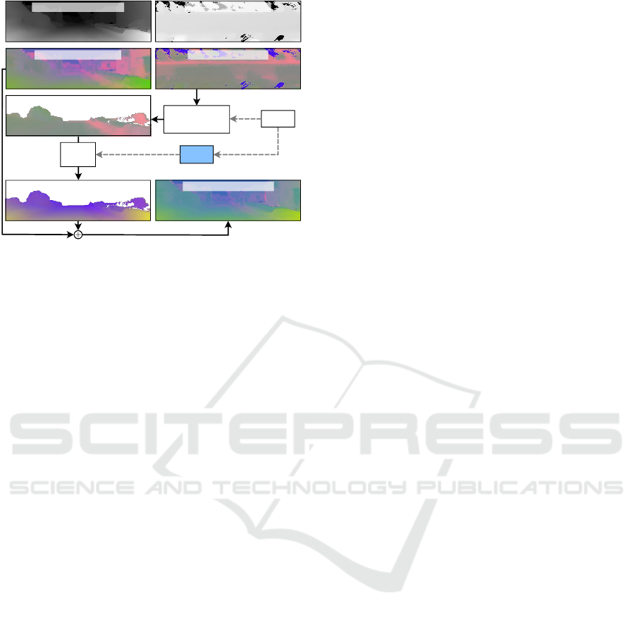
Aggregated feature-map

MLP

1×1

Conv

front,top

Front view inverse-depth Top view inverse-depth

Front view feature-map Top view feature-map

Warped top-view

feature-map

Warped and transformed top-view

feature-map

Feature space

reprojection

Feature Map

Warping

Aggregate

Figure 1: Feature map aggregation. In the top two rows we

show inverse-depth images for a front and a top view, along

with two feature maps. To aggregate the feature map of the

top view with the front view, we ﬁrst warp the top feature

map into the front view. The relative transform between the

top and the front view,

f ront,top

, is processed by a multi-

layer perceptron (

MLP

) to generate a linear transform that

maps the features from the top to the front view. Finally, the

resulting feature map can be aggregated with the front view

feature map. Note that in the front feature map the features

fade from green to violet, while in the warping of the top

view, the features do not change with depth towards the

horizon until after transforming the features. The front view

feature maps are aggregated analogously. For visualisation,

the above feature maps are projected to three channels using

the same random projection.

We apply this method to the problem of correcting

dense meshes. We render 2D views from recon-

structions and learn how to reﬁne inverse-depth,

while making use of multi-view information.

In our experiments we look at two ways of aggre-

gating feature maps and conclude that the feature space

transformation is necessary to beneﬁt from the use of

multiple views when correcting reconstructions.

2 RELATED WORK

Our work focuses on reﬁning the output of an existing

reconstruction system such as BOR

G (Tanner et al.,

2015) or KinectFusion (Newcombe et al., 2011), thus

producing higher-quality reconstructions. Since we

achieve this by operating on 2D projections and re-

ﬁning inverse-depth, our work is related to depth re-

ﬁnement. In the following we summarise some of the

related literature and methods used in this work.

Mesh Correction.

(Tanner et al., 2018) ﬁrst propose

ﬁxing reconstructions by reﬁning 2D projections of

them with a

CNN

, one at a time. The geometrical

relation between neighbouring views is leveraged by

aftescu and Newman, 2020) during training, by the

addition of a geometric consistency loss that penalises

differences in geometry. In this work, we process

neighbouring views jointly not only while training, but

also when making predictions.

Learnt Depth Reﬁnement and Completion.

There

are several depth reﬁnement methods similar to our ap-

proach. Multiple depth maps are fused by (Kwon et al.,

2015) with KinectFusion (Newcombe et al., 2011) to

obtain a high-quality reference mesh and use dictio-

nary learning to reﬁne raw RGB-D images. Using

CNN

on the colour channels of an RGB-D image,

(Zhang and Funkhouser, 2018) predict normals and oc-

clusion boundaries and use them to optimise the depth

component, ﬁlling in holes. In the method proposed by

(Jeon and Lee, 2018), depth images are rendered from

a reconstruction at the same locations as the raw depth,

obtaining a 4000-image dataset of raw/clean depth im-

age pairs. The authors train a

CNN

to reﬁne the raw

depth maps, and show that using it reduces the amount

of data and time needed to build reconstructions. All

of these methods require a colour image in order to

reﬁne depth, and operate on live data, which limits

the amount of training data available. In contrast, our

method is designed to operate post-hoc, on existing

meshes. We can therefore generate an arbitrary num-

ber of training pairs from any viewpoint, removing any

viewpoint-speciﬁc bias that might otherwise surface

while learning.

Another recent approach proposes depth reﬁne-

ment by fusing feature maps of neighbouring views

through warping (Donne and Geiger, 2019). While

this is similar to our approach, we take the additional

step of transforming the features between views, and

consider two feature aggregation methods.

Dynamic Filter Networks.

Generating ﬁlters for

convolutions dynamically conditioned on network in-

puts is presented by (Brabandere et al., 2016), where

ﬁlters are predicted for local spatial transforms that

help in video prediction tasks. Our feature transforma-

tion is also based on this framework: given a relative

transform between two views, we predict the weights

that would transform features from one view to another.

A key distinction is that, while the ﬁlters in the origi-

nal work are demonstrated over the spatial domain, we

operate solely on the channels of the feature map with

a 1 ×1 convolution.

VISAPP 2021 - 16th International Conference on Computer Vision Theory and Applications

902

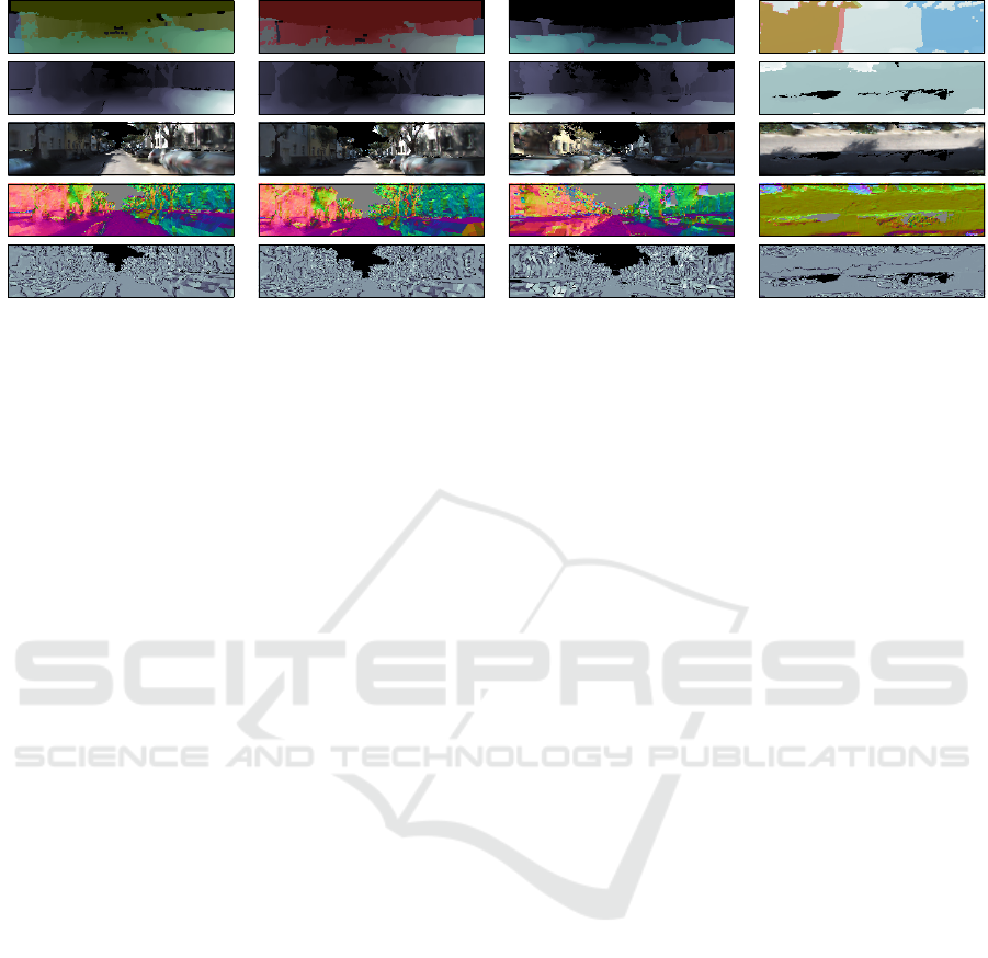
(a) Left (b) Right (c) Back (d) Top

Figure 2: Example of training data generated from a 3D mesh. Each column represents a different view rendered around the

same location. The top row shows the inverse-depth images rendered from the lidar reconstruction, with areas visible in the

other views shaded: red for left, green for right, blue for back, and cyan for top. The next four rows show the mesh features we

render from the stereo camera reconstruction: inverse-depth, colour, normals, and triangle surface area. Our proposed model

learns to reﬁne the low-quality inverse-depth (second row), using the rendered mesh features (rows 2–5) as input, processing all

four views jointly, and supervised by the high-quality inverse-depth label (ﬁrst row).

3 METHOD

3.1 Training Data

Our main goal is to correct existing dense reconstruc-

tions. To bypass the need for expensive computation,

we operate on 2D projections of a mesh from multiple

viewpoints. As we want to capture as much of the

geometry as possible in our projections, we render sev-

eral mesh features for each viewpoint: inverse-depth,

colour, normals, and triangle surface area (see Fig-

ure 2).

During training, we have access to two reconstruc-

tions of the same scene: a low-quality one that we learn

to correct, and a high-quality one that we use for super-

vision. In particular, we learn to correct stereo-camera

reconstructions using lidar reconstructions as supervi-

sion. Figure 3 shows an overview of our method.

The ground-truth labels,

∆

, are computed as the

difference in inverse-depth between high-quality and

low-quality reconstructions:

∆(p) = d

(p) −d

(p) (1)

where

is a pixel index, and

and

are inverse-

depth images for the high-quality and low-quality re-

construction, respectively. For notational compactness,

∆(p)

is referred to as

∆

, and future deﬁnitions are over

all values of p, unless otherwise speciﬁed.

There are several advantages to using inverse-

depth. Firstly, geometry closer to the camera will

have higher values and therefore these areas will be

emphasised during training. Secondly, inverse-depth

smoothly fades away from the camera, such that the

background – which has no geometry and is inﬁnitely

far away – has a value of zero. If we were to use

depth, we would have to treat background as a spe-

cial case, since neural networks are not equipped to

deal with inﬁnite values out-of-the-box. Finally, when

warping images from one viewpoint from another, as

described in the following sections, we are in essence

re-sampling. To correctly interpolate depth values, we

would have to use harmonic mean, which is less nu-

merically stable, whereas interpolating inverse-depth

can be done linearly.

3.2 Image Warping

During both training and prediction, we need to fuse

information from neighbouring views. While training,

we want to penalise the network for making predictions

that are geometrically inconsistent between views, us-

ing the geometric consistency loss from (S

aftescu and

Newman, 2020), described in Section 3.3.4. When

making predictions, we want to be able to aggregate

information from multiple views. To enable this, we

need to warp images between viewpoints, such that

corresponding pixels are aligned.

Consider a view

, an inverse-depth image

, and

a pixel location within the image,

= [u v 1]

. The

homogeneous point corresponding to p

is:



−1

)



, (2)

where

is the camera intrinsic matrix. Consider fur-

ther a nearby view

, an image

, and the relative

Learning to Correct Reconstructions from Multiple Views

903

transform

n,t

∈ SE(3)

from

that maps points

between views:

= T

n,t

. The pixel in view

corre-

sponding to p

is:

= K

(1:3)

(3)

, (3)

where a superscript indexes into the vector x

We can now warp image I

into view t:

t←n

) = I

). (4)

Note here that

might not have integer values, and

therefore might not lie exactly on the image grid of

In that case, we linearly interpolate the nearest pixels.

Since the value of inverse-depth is view-dependent,

when warping inverse-depth images we make the fol-

lowing additional deﬁnition:

t;n

) =

(4)

(3)

, (5)

which represents an image aligned with view

, with

inverse-depth values in the frame of n.

Occlusions.

Pixel correspondences computed

through warping are only valid where there are no

occlusions. We therefore have need of a mask to only

take into account unoccluded regions. Therefore,

when rendering mesh features, we also render an

additional image where every pixel is assigned

the ID of the visible mesh triangle at that location.

The triangle ID is computed by hashing the global

coordinates of its vertices. We can then warp this

image of triangle IDs from the source to the target

view. If the ID of a pixel matches between the warped

source and the target image, we know that the same

surface is in view in both images – and thus that pixel

is unoccluded.

3.3 Network Architecture

3.3.1 Model

We use an encoder-decoder architecture, with asym-

metric ResNet (He et al., 2016) blocks, the sub-pixel

convolutional layers proposed by (Shi et al., 2016)

for upsampling in the decoder, and skip connections

between the encoder and the decoder to improve sharp-

ness, as introduced by the U-Net architecture (Ron-

neberger et al., 2015). Throughout the network, we

use ELU (Clevert et al., 2015) activations and group

normalisation (Wu and He, 2018). Table 1 details the

blocks used in our network. We use F = 8 input chan-

nels: 3 for colour, 3 for normals, 1 for inverse-depth,

and 1 for triangle area.

Table 1: Overview of the

CNN

architecture for error predic-

tion.

Block Type

Filter Size

/ Stride

Output Size

Input - 96 × 288 × F

Projection 7 × 7/1 96 × 288 × 16

Residual 3 × 3/1 96 × 288 × 16

Projection, Residual×2 3 × 3/2 48 × 144 × 32

Projection, Residual×2 3 × 3/2 24 × 72 × 64

Projection, Residual×2 3 × 3/2 12 × 36 × 128

Projection, Residual×5 3 × 3/2 6 × 18 × 256

Up-projection, Skip 3 × 3/

12 × 36 × 384

Up-projection, Skip 3 × 3/

24 × 72 × 192

Up-projection, Skip 3 × 3/

48 × 144 × 96

Up-projection, Skip 3 × 3/

96 × 288 × 48

Residual×2 3 × 3/1 96 × 288 × 48

Convolution 3 × 3/1 96 × 288 × 1

Since a fair portion of the input low-quality re-

construction is already correct, we train our model to

predict the error in the input inverse-depth,

∆

∗

. We

then compute the reﬁned inverse depth as the output

of our network:

∗

= max(d

+ ∆

∗

,0). (6)

Clipping is required here because inverse-depth

cannot be negative. However, since we are supervising

the predicted error, the network can learn even when

the predicted inverse-depth is clipped and would there-

fore lack a gradient. To ensure our network can deal

with any range of inverse-depth, we offset the input

such that it has zero mean, scale it to have standard

deviation of 1, and undo the scaling on the predicted

error, ∆

∗

3.3.2 Feature Map Warping and Aggregation

As our predictions are related by the geometry of a

scene, we must would like to ensure predictions are

consistent between views. This is taken into account

during training by using the geometric consistency loss

from (S

aftescu and Newman, 2020), as described in

Section 3.3.4.

However, during inference we would like to ag-

gregate information from multiple views to improve

predictions. Take, for example, two views,

and

and feature maps in the network,

and

, after a

certain number of layers, corresponding to each of

the views. We would like to aggregate them such that

⊕ F

is a feature map containing information from

both views. Since the feature maps are aligned with

the input views, we cannot do that in a pixel-wise fash-

ion. Using the input depth, we warp the feature map

of one view into the frame of the other, such that the

input geometry is aligned. For the two input views, we

VISAPP 2021 - 16th International Conference on Computer Vision Theory and Applications

904

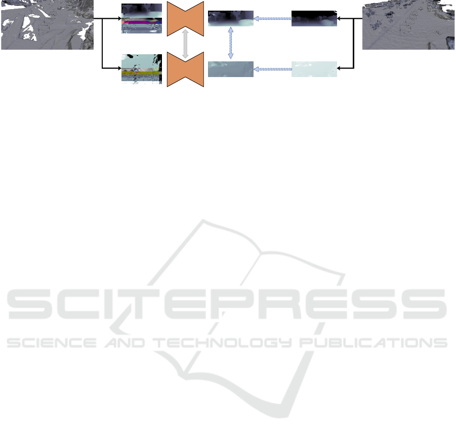
Geometric

Consistency

Regression

(data, ∇)

Regression

(data, ∇)

Rened

Inverse-depth

CNN

Feature Map

Aggregation

Extracted

mesh features

Inverse-depth

labels

Stereo Reconstruction

Lidar Reconstruction

Figure 3: Illustration of our training set-up. Starting with a low-quality reconstruction (stereo camera in this instance), we

extract mesh features from several viewpoints. Our network learns to reﬁne the input inverse-depth with supervision from a

high-quality (lidar) reconstruction. The blue arrows above indicate the losses used during training: for each view, we regress to

the high-quality inverse-depth, as well as to its gradient; between nearby prediction, we apply a geometric consistency loss to

encourage predictions with the same geometry. Within the network, feature maps are aggregated between views so information

can propagate within a neighbourhood of views, as illustrated in a two-view case in Figure 1. Adapted with permission from

aftescu and Newman, 2020).

can thus warp

to the viewpoint of

(according to

Equation 4) and then aggregate the two feature maps:

t,n

= F

⊕ F

t←n

, obtaining a feature map aligned with

t that combines information from both views.

This aggregation step is necessary (instead of sim-

ply concatenating aligned feature maps) to allow for

an arbitrary number of views. For the same reason, the

aggregation function needs to be invariant to permu-

tations of views. We consider two such aggregation

functions: averaging, and attention. For a target view

with neighbourhood

N = {t} ∪ {n

,...}

, averag-

ing is deﬁned as

∑

n∈N

t←n

/|N|

, where we consider

t←t

≡ F

For the attention-based aggregation, we use the

attention method proposed by (Bahdanau et al., 2014).

A per-pixel score

t,n

= a(F

t←n

)

is computed using

a small 3-layer convolutional sub-network. The per-

pixel weight of each view is obtained by applying soft-

max to the scores:

t,n

= exp(E

t,n

∑

m∈N

exp(E

t,m

)

Finally, the aggregation function becomes

∑

n∈N

t,n

t←n

. In both cases, pixels deemed occluded are

masked out.

In our model, we apply this warping and aggrega-

tion to every skip connection and to the encoder output,

thus mixing information across views and scales. For

every view in a batch, we aggregate all the other over-

lapping views within the batch.

3.3.3 Feature Space Reprojection

When the network is trained to make predictions one

input view at a time, the feature maps at intermediate

layers within the network contain viewpoint-dependent

features, as illustrated in Figure 1. Warping a feature

map from one view to another only aligns features

using the scene geometry, but does not change their

dependence on viewpoint.

Imagine, for example, two RGB-D images in an

urban scene – one from above looking down, and one

at the road level. The surface of the road will have

the same colour in both views. The depth of the road,

however, will be different: in the top view, it will be

mostly uniform, while in the road-level view it will

increase towards the horizon. We can easily establish

correspondences between pixels in the two images

if we know their relative pose. When not occluded,

corresponding pixels will have the same colour, but

not necessarily the same depth. This is because colour

is view-point independent, while depth depends on the

viewpoint. In other words, we can resample the colour

from one view to obtain the other view by directly

indexing and interpolating (as in Equation 4), while for

depth we also need to transform the values of the ﬁrst

view to match the reference frame of the second view

(as in Equation 5). Armed with this observation we

propose a way to learn a mapping of features between

viewpoints.

Consider again two views

and

, and a warped

feature map

t←n

from the vantage point

. Given

a spatial location

, we have a feature vector

t←n

(p) ∈ R

, its corresponding location in space

= (x,y,z, w) ∈ P

, and a transform

t,n

∈ SE(3)

We compute a matrix

W = g(T

t,n

) ∈ M

D,D+4

, using a

small multi-layer perceptron (

MLP

) to model

. This

allows us to learn a linear transform in feature space

between view n and view t:

= W





. (7)

Without this mechanism, the network would have to

learn to extract viewpoint-independent features to al-

low for feature aggregation between views.

Concretely, we implement this as a dynamic ﬁlter

network (

DFN

), with a 4-layer

MLP

generating ﬁlters

for a

1 × 1

linear convolution of the warped feature

map

t←n

, which is equivalent to applying the multi-

plication in Equation 7 at every spatial location in the

feature map. To keep the

MLP

small, we ﬁrst project

Learning to Correct Reconstructions from Multiple Views

905

(a) Sequence 00 (b) Sequence 05 (c) Sequence 06

Figure 4: Illustration of the training (blue), validation (orange), and test (green) splits on the three

KITTI-VO

sequences we are

using. Map data copyrighted (OpenStreetMap contributors, 2017) and available from https://www.openstreetmap.org.

the input feature maps to

D = 32

dimensions, apply the

dynamically generated ﬁlters, and then project back

to the desired number of features. Both projections

are implemented using

1 × 1

convolutions. We use the

same transformation

across each of the the scales

that we aggregate, and all the weights associated with

feature transform operations are learnt jointly with the

rest of the weights of the network.

In the experiments, we show that this mechanism is

essential for enabling effective multi-view aggregation.

3.3.4 Loss Function Formulation

We supervise our training with labels from a high-

quality reconstruction, as sown in Figure 3. The labels

provide two per-pixel supervision signals, one for di-

rect regression,

dat a

, and one for prediction gradients,

∇

dat a

∑

p∈V

∆

∗

− ∆

berHu

; (8)

∇

∑

p∈V



∂

∆

∗

− ∂

∆



∂

∆

∗

− ∂

∆





, (9)

where

is the set of valid pixels (to account for miss-

ing data in the ground-truth),

∆

∗

and

∆

are the pre-

diction and the target, respectively, and

k · k

berHu

the berHu norm (Owen, 2007), whose advantages for

depth prediction have been explored by (Laina et al.,

2016; Ma and Karaman, 2018). We use the Sobel op-

erator (Sobel and Feldman, 1968) to approximate the

gradients in Equation 9.

The geometric consistency loss guides nearby pre-

dictions to have the same geometry, and relies on

warped nearby views

∗

t←n

. For a target view

, a set

of nearby views

, the set of pixels unoccluded in a

nearby view

(see Figure 2, top row), this loss is

deﬁned as:

∑

n∈N

∑

p∈U



∗

t←n

−

∗

t;n



. (10)

Both

∗

t←n

and

∗

t;n

are aligned with view

and contain

inverse-depth values in frame

, as per Equation 4

and Equation 5. Note that

has no relation to the

set of valid pixels (

) from the previous losses, since

this loss is only computed between predictions. This

enables the network to make sensible predictions even

in parts of the image which have no valid label.

Finally, we also include an

weight regulariser,

reg

, to reduce overﬁtting by keeping the weights

small. The overall objective is thus deﬁned as:

L = λ

dat a

+ λ

∇

+ λ

reg

, (11)

where the

s are weights for each of the components.

We use

dat a

= 1

∇

= 0.1

, and

reg

−6

4 EXPERIMENTS

4.1 Experimental Setup

4.1.1 Dataset

For the experiments, we use sequences “00”, “05”,

and “06” from the KITTI visual odometry (

KITTI-VO

)

dataset (Geiger et al., 2013). Using the BOR

G recon-

struction system (Tanner et al., 2015), we create pairs

of low/high quality reconstructions (meshes) from the

stereo camera, and lidar, respectively. Following the

same trajectory used when collecting data (as it is

collision-free), every 0.65 m we render mesh features

from four views (left, right, back, top), illustrated in

Figure 2. For each view, we render a further 3 sam-

ples with small pose perturbations for data augmenta-

tion. In total, we obtain 178 544 distinct views of size

96 × 288 over 7.2 km.

4.1.2 Training and Inference

We train all our models on Nvidia Titan V GPUs, using

the Adam optimiser (Kingma and Ba, 2015), with

= 0.9

= 0.999

, and a learning rate that decays

linearly from

−4

5 · 10

−6

over 120 000 training

steps. We clip the gradient norm to 80. Each training

VISAPP 2021 - 16th International Conference on Computer Vision Theory and Applications

906

Table 2: Depth Error Correction Results.

Model iMAE iRMSE δ < 1.05 δ < 1.15 δ < 1.25 δ < 1.56 δ < 1.95

Uncorrected 1.21 · 10

−2

3.80 · 10

−2

51.92% 82.44% 86.66% 90.54% 91.97%

Baseline 7.09 · 10

−3

2.47 · 10

−2

73.81% 89.33% 93.08% 96.71% 97.98%

Ours (no feat. tf.; avg.) 7.11 · 10

−3

2.45 · 10

−2

72.70% 89.08% 92.87% 96.53% 97.86%

Ours (no feat. tf.; attn.) 7.22 · 10

−3

2.52 · 10

−2

73.60% 89.18% 92.90% 96.57% 97.87%

Ours (w/ feat. tf.; avg.) 6.82 · 10

−3

2.38 · 10

−2

74.22% 90.01% 93.51% 96.79% 98.01%

Ours (w/ feat. tf.; attn.) 6.88 · 10

−3

2.40 · 10

−2

74.34% 89.85% 93.47% 96.89% 98.10%

Table 3: Generalisation Capability of Depth Error Correction.

Model Train Test iMAE iRMSE δ < 1.05 δ < 1.15 δ < 1.25 δ < 1.56 δ < 1.95

Uncorrected – 06 2.43 · 10

−2

8.39 · 10

−2

49.63% 72.89% 75.07% 78.48% 80.23%

Baseline 00; 05 06 2.09 · 10

−2

8.21 · 10

−2

59.99% 79.16% 82.62% 86.33% 88.54%

Ours (no feat. tf.) 00; 05 06 2.06 · 10

−2

8.11 · 10

−2

61.57% 77.95% 81.46% 85.45% 87.88%

Ours (w/ feat. tf.) 00; 05 06 1.94 · 10

−2

6.80 · 10

−2

63.90% 78.80% 82.00% 85.80% 88.04%

Uncorrected – 05 1.15 · 10

−2

3.59 · 10

−2

55.85% 81.60% 85.07% 88.86% 90.90%

Baseline 00; 06 05 7.76 · 10

−3

2.98 · 10

−2

72.23% 87.54% 91.23% 95.46% 97.41%

Ours (no feat. tf.) 00; 06 05

7.79 · 10

−3

2.97 · 10

−2

71.57% 87.20% 90.94% 95.31% 97.34%

Ours (w/ feat. tf.) 00; 06 05 7.65 · 10

−3

2.96 · 10

−2

73.24% 87.61% 91.16% 95.34% 97.29%

Uncorrected – 00 1.19 · 10

−2

3.24 · 10

−2

53.53% 80.46% 85.18% 89.55% 91.38%

Baseline 05; 06 00 8.40 · 10

−3

2.50 · 10

−2

67.52% 86.83% 91.28% 95.85% 97.70%

Ours (no feat. tf.) 05; 06 00 8.32 · 10

−3

2.49 · 10

−2

66.04% 86.65% 91.34% 95.80% 97.64%

Ours (w/ feat. tf.) 05; 06 00 8.40 · 10

−3

2.53 · 10

−2

67.90% 87.02% 91.39% 95.83% 97.64%

batch contains 4 different examples, and each example

is composed of the four views rendered around a single

location. Unless otherwise mentioned, we train our

models for 500 000 steps. During inference, our full

model runs at 11.3 Hz when aggregating 4 input views,

compared to the baseline that runs at 12.6 Hz, so our

method comes with little computational overhead.

4.1.3 Metrics

As our method operates on 2D views extracted from

the mesh we are correcting, we measure how well

our network predicts inverse-depth images, with the

idea that better inverse-depth images result in better

reconstructions. We employ several metrics common

in the related tasks of depth prediction and reﬁnement.

One way to quantify performance is to see how of-

ten the error in prediction is small enough to be correct.

The thresholded accuracy measure is essentially the

expectation that a given pixel is within a fraction

thr

of the label:

δ = E

p∈V





max



∗



< thr



, (12)

where

is the reference inverse-depth,

∗

is the

predicted inverse depth,

is the set of valid pix-

els,

is the cardinality of

, and

I(·)

represents the

indicator function. For granularity, we use

thr ∈

{1.05,1.15,1.25,1.25

,1.25

In addition, we also compute the mean absolute er-

ror (

MAE

) and root mean square error (

RMSE

) metrics

to quantify per pixel error:

iMAE =

∑

p∈V



∗

− d



, (13)

iRMSE =

∑

p∈V

∗

− d

)

, (14)

where the ‘i’ indicates that the metrics are computed

over inverse-depth images.

4.2 Gross Error Correction

For the ﬁrst set of experiments, we take the ﬁrst 80%

of the views from each sequence as training data, the

next 10% for validation, and show our results on the

last 10%. An illustration of the KITTI sequences and

splits is shown in Figure 4.

As baseline, we train our model with geometric

consistency loss but without any feature aggregation.

During inference, this model makes predictions one

view at a time.

To illustrate our method, we train a further two

models for each aggregation method (averaging and

Learning to Correct Reconstructions from Multiple Views

907

attention): one with the feature transform disabled,

and one with it enabled.

As it can be seen in Table 2, the baseline already

reﬁnes inverse-depth signiﬁcantly. Without our feature

transformation, the models are unable to use multi-

view information because of the vastly different view-

points, and indeed this slightly hurts performance.

Only when transforming the features between view-

points does the performance increase over the baseline,

highlighting the importance of our method for success-

fully aggregating multiple views.

4.3 Generalisation

To asses the ability of our method to generalise on

unseen reconstructions, we divide our training data by

sequence: we use two of the sequences for training,

and the third for testing. Sequences 00 and 05 are

recorded in a suburban area with narrow roads, while

sequence 06 is a loop on a divided road with a median

strip, a much wider and visually distinct space. We

train models for 200 000 steps and aggregate feature

maps by averaging. The results in Table 3 show that

our method successfully uses information from mul-

tiple views, even in areas of a city different from the

ones it was trained on. Furthermore, they reafﬁrm the

need for our feature transformation method in addition

to warping.

5 CONCLUSION AND FUTURE

WORK

In conclusion, we have presented a new method for

correcting dense reconstructions via 2D mesh feature

renderings. In contrast to previous work, we make pre-

dictions on multiple views at the same time by warping

and aggregating feature maps inside a

CNN

. In addi-

tion to warping the feature maps, we also transform the

features between views and show that this is necessary

for using arbitrary viewpoints.

The method presented here aggregates feature

maps between every pair of overlapping input views.

This scales quadratically with the number of views

and thus limits the size of the neighbourhood we can

reasonably process. Future work will consider aggre-

gation into a shared 2D spatial representation, such as

360

◦

view, which would scale linearly with the input

neighbourhood size.

While in this paper we have applied our method

to correct stereo reconstructions using lidar as high-

quality supervision, our approach operates strictly on

meshes, so it is agnostic to the types of sensors used

to produce the low- and high-quality reconstructions,

so long as it is trained accordingly.

REFERENCES

Bahdanau, D., Cho, K., and Bengio, Y. (2014). Neural

machine translation by jointly learning to align and

translate. In Proceedings of The International Confer-

ence on Learning Representations (ICLR).

Brabandere, B. D., Jia, X., Tuytelaars, T., and Gool, L. V.

(2016). Dynamic ﬁlter networks. In Proceedings of The

Conference on Neural Information Processing Systems

(NIPS).

Clevert, D.-A., Unterthiner, T., and Hochreiter, S. (2015).

Fast and accurate deep network learning by exponen-

tial linear units (ELUs). In Proceedings of The In-

ternational Conference on Learning Representations

(ICLR).

Donne, S. and Geiger, A. (2019). Defusr: Learning non-

volumetric depth fusion using successive reprojections.

In Proceedings of The IEEE/CVF International Con-

ference on Computer Vision and Pattern Recognition

(CVPR).

Geiger, A., Lenz, P., Stiller, C., and Urtasun, R. (2013).

Vision meets robotics: The kitti dataset. The Inter-

national Journal of Robotics Research, 32(11):1231–

1237.

He, K., Zhang, X., Ren, S., and Sun, J. (2016). Deep resid-

ual learning for image recognition. In Proceedings

of The IEEE/CVF International Conference on Com-

puter Vision and Pattern Recognition (CVPR), pages

770–778.

Jeon, J. and Lee, S. (2018). Reconstruction-based pairwise

depth dataset for depth image enhancement using CNN.

In Proceedings of The European Conference on Com-

puter Vision (ECCV).

Kingma, D. and Ba, J. (2015). Adam: A method for stochas-

tic optimization. In Proceedings of The International

Conference on Learning Representations (ICLR).

Kwon, H., Tai, Y.-W., and Lin, S. (2015). Data-driven depth

map reﬁnement via multi-scale sparse representation.

In Proceedings of The IEEE/CVF International Con-

ference on Computer Vision and Pattern Recognition

(CVPR), pages 159–167.

Laina, I., Rupprecht, C., Belagiannis, V., Tombari, F., and

Navab, N. (2016). Deeper depth prediction with fully

convolutional residual networks. In Proceedings of The

IEEE International Conference on 3D Vision (3DV),

pages 239–248.

Ma, F. and Karaman, S. (2018). Sparse-to-dense: Depth pre-

diction from sparse depth samples and a single image.

In Proceedings of The IEEE International Conference

on Robotics and Automation (ICRA).

Newcombe, R. A., Izadi, S., Hilliges, O., Molyneaux, D.,

Kim, D., Davison, A. J., Kohli, P., Shotton, J., Hodges,

S., and Fitzgibbon, A. W. (2011). KinectFusion: Real-

time dense surface mapping and tracking. In Proceed-

ings of The IEEE International Symposium on Mixed

and Augmented Reality (ISMAR), pages 127–136.

VISAPP 2021 - 16th International Conference on Computer Vision Theory and Applications

908

OpenStreetMap contributors (2017). Planet dump re-

trieved from https://planet.osm.org. https://www.

openstreetmap.org.

Owen, A. B. (2007). A robust hybrid of lasso and ridge

regression. Contemporary Mathematics, 443:59–72.

Ronneberger, O., Fischer, P., and Brox, T. (2015). U-Net:

Convolutional networks for biomedical image segmen-

tation. In Medical Image Computing and Computer

Assisted Intervention (MICCAI).

Shi, W., Caballero, J., Husz

ar, F., Totz, J., Aitken, A. P.,

Bishop, R., Rueckert, D., and Wang, Z. (2016). Real-

time single image and video super-resolution using

an efﬁcient sub-pixel convolutional neural network.

In Proceedings of The IEEE/CVF International Con-

ference on Computer Vision and Pattern Recognition

(CVPR), pages 1874–1883.

Sobel, I. and Feldman, G. (1968). A 3

3 isotropic gradi-

ent operator for image processing. presented at the

Stanford Artiﬁcial Intelligence Project (SAIL).

aftescu,

. and Newman, P. (2020). Learning geometrically

consistent mesh corrections. In Proceedings of The

International Conference on Computer Vision Theory

and Applications (VISAPP).

Tanner, M., Pini

es, P., Paz, L. M., and Newman, P. (2015).

BOR

G: Building optimal regularised reconstructions

with GPUs (in cubes). In Proceedings of The Interna-

tional Conference on Field and Service Robotics (FSR),

Toronto, Canada.

Tanner, M., S

aftescu,

., Bewley, A., and Newman, P. (2018).

Meshed up: Learnt error correction in 3D reconstruc-

tions. In Proceedings of The IEEE International Con-

ference on Robotics and Automation (ICRA), Brisbane,

Australia.

Wu, Y. and He, K. (2018). Group normalization. In Proceed-

ings of The European Conference on Computer Vision

(ECCV).

Zhang, Y. and Funkhouser, T. A. (2018). Deep depth comple-

tion of a single RGB-D image. In Proceedings of The

IEEE/CVF International Conference on Computer Vi-

sion and Pattern Recognition (CVPR), pages 175–185.

Learning to Correct Reconstructions from Multiple Views

909