Multimodal Neural Network for Sentiment Analysis in Embedded

Systems

Quentin Portes

, Jos

e Mend

es Carvalho

, Julien Pinquier

and Fr

eric Lerasle

Renault Software Lab, Toulouse, France

IRIT, Paul Sabatier University, CNRS, Toulouse, France

LAAS-CNRS, Paul Sabatier University, Toulouse, France

Keywords:

Sentiment Analysis, Deep Learning, Multimodal, Fusion, Embedded System, Cockpit Monitoring.

Abstract:

Multimodal neural network in sentiment analysis uses video, text and audio. Processing these three modalities

tends to create computationally high models. In the embedded context, all resources and speciﬁcally compu-

tational resources are restricted. In this paper, we design models dealing with these two antagonist issues. We

focused our work on reducing the numbers of model input features and the size of the different neural network

architectures. The major contribution in this paper is the design of a speciﬁc 3D Residual Network instead

of using a basic 3D convolution. Our experiments are focused on the well-known dataset MOSI (Multimodal

Corpus of Sentiment Intensity). The objective is to perform similar results as the state of the art. Our best

multimodal approach achieves a F1 score of 80% with a number of parameters reduced by 2.2 and the memory

load reduced by a factor 13.8, compared to the state of the art. We designed ﬁve models, one for each modality

(i.e video, audio and text) and one for each fusion technique. The two high-level multimodal fusions presented

in this paper are based on the evidence theory and on a neural network approach.

1 INTRODUCTION

Sentiment analysis remains a recent subject of study,

99% of publications on this topic have been published

after 2004. The reader can refer to (M

antyl

a et al.,

2018) for a complete review on this modality subject.

Sentiment analysis is used in diverse ﬁelds of appli-

cation. Today, companies like Facebook, Amazon or

Twitter infer sentiment analysis thanks to the massive

amount of data uploaded every day on their servers.

These companies mainly adopt this type of data to ex-

tract the opinion expressed in the video stream or text

stream. More speciﬁcally they use these technologies

for brand monitoring, customer service, market re-

search, and analysis (Benedetto and Tedeschi, 2016;

Greco and Polli, 2020). Recent studies show the efﬁ-

ciency of text sentiment analysis on tweets or even on

Amazon product reviews (Trupthi et al., 2017; Nandal

et al., 2020).

Plethora of applications can today be enhanced

with deep learning. Smartphones employ IA for the

unlocking system (Baqeel and Saeed, 2019). They

also use IA to sublimate picture quality (Vu et al.,

2019). Recent cars use IA for pedestrian detec-

tions (Shi et al., 2020) or road sign detections (Dubey

et al., 2020). New headphones also implement IA

to reduce environmental noise (Reshma and Kiran,

2017). These new technologies embed dedicated IA

software and hardware. These types of tasks can be

difﬁcult to execute on a server, mainly because of

the necessity to have an Internet connection. Two

particular problems are intensiﬁed when an Internet

connection is needed: latency between the server

and the client and data leak. With the current craze

for IA, component manufacturers attend today to de-

sign modern hardware to execute deep learning algo-

rithms. This recent development is inevitable because

of the high computing resources required by IA. It in-

volves the use of expensive hardware. One of the so-

lutions to not increase the ﬁnal price of the product is

to adapt IA models to cheaper hardware.

In the automotive ﬁeld, sentiment analysis is a ma-

jor issue. For example, the level of satisfaction of the

driver in the cockpit can be analyzed. It is also possi-

ble to study the interactions between the driver and the

Human Machine Interface (HMI) of the board com-

puter. With the challenge of autonomous vehicles, the

driver will have to regularly take control over a vehi-

cle moving in the trafﬁc. The difﬁculties for the driver

are to maintain a suitable awareness of the situation to

Portes, Q., Carvalho, J., Pinquier, J. and Lerasle, F.

Multimodal Neural Network for Sentiment Analysis in Embedded Systems.

DOI: 10.5220/0010224703870398

In Proceedings of the 16th International Joint Conference on Computer Vision, Imaging and Computer Graphics Theory and Applications (VISIGRAPP 2021) - Volume 5: VISAPP, pages

387-398

ISBN: 978-989-758-488-6

387

take back the task of driving. (W

orle et al., 2020)

investigate the conducting behavior of drivers after

sleeping. The idea is to have a maximum of data on

the driver and passenger states to suggest beneﬁcial

actions and information to assist the driver. In other

contexts, like ﬂeet of autonomous vehicles, without

any driver in the vehicle, the critical problem is the

lack of authority. By analyzing the levels of interac-

tion inside the car we could detect incidents like ag-

gression and then trigger an alarm to inform a remote

controller.

Regardless of the industrial application, embed-

ded resources are always limited. Even with powerful

hardware, the performance of a Deep Neural Network

remains limited by three factors: memory bandwidth,

math bandwidth, and latency. Note T

memory

time spent

in accessing memory and T

math

time spent performing

math operations. On a given processor a given algo-

rithm is math limited if T

math

> T

memory

Expressed:

ops

bytes

math

memory

(1)

with ops the operations and BW the bandwidth.

In an embedded environment, those three factors

are more constrained than servers or computer ma-

chines. The three previous factors are directly im-

pacted by the three following operations:

• Element-wise operations.

• Reduction operations.

• Dot-Product operations.

When we deal with embedded systems, two hardware

components are directly impacted by the size of the

model:

• CPU and/or GPU loading.

• Memory loading.

Today, in image analysis the tendency is to deeply

modify the architecture to tune model for the smart-

phones or embedded devices. The objective is to

reduce CPU computation while improving perfor-

mances. Recent works in object recognition show

huge improvements in reducing the CPU/GPU re-

sources of the neural network model (Bochkovskiy

et al., 2020; Howard et al., 2019). Embed this deep

learning model remain a technological challenge.

Given these insights, this paper focuses on de-

signing a model with equivalent performances to the

state-of-the-art (or higher), but with computational re-

sources drastically reduced. We differ from the lit-

erature by the embedded approach in the context of

sentiment analysis, which is, to our best knowledge

marginally studied. Our approach also differs by our

concrete ultimate objective which is to embed our

model in a vehicle by minimizing the CPU/GPU re-

sources required. We privilege a public dataset in or-

der to compare our performances with the literature

while improving drastically the model compactness.

The paper is organized as follows. Section 2 intro-

duces a literature review on multimodality sentiment

analysis. In section 3, we expose the methodology

on each modality and our multimodal approach. Sec-

tion 4 provides information on dataset and experimen-

tal results.

2 RELATED WORKS

Most sentiment analysis approaches are only based

on text due to the high availability of text datasets,

like (Maas et al., 2011) or Amazon and Tweeter

datasets. Recent studies, with new approaches such

as multimodality, show the beneﬁt of exploiting infor-

mation from different channels. All multimodal mod-

els on sentiment analysis ﬁelds outperform unimodal

architectures (Poria et al., 2017; Cambria et al., 2017;

Huddar et al., 2018; Agarwal et al., 2019). These

methods are based on feature level fusion, which

means that features are extracted from three differ-

ent modalities (i.e the video, audio and text). Then, a

more or less complex late fusion is applied.

OpenSMILE (Eyben et al., 2010) is often used

for the audio modality (Poria et al., 2017; Cambria

et al., 2017; Huddar et al., 2018). It is an open-source

software that extracts high and low-level features like

pitch, voice intensity, MFCC, etc. The more com-

plex task is to determine the best numbers of features

that should be used to get the best score. Approaches

of (Poria et al., 2017) and (Cambria et al., 2017) use

6373 features which is too much for an embedded so-

lution. On the contrary, (Huddar et al., 2018) use only

991 features which is more realistic in our application

context.

On the text analysis two methods are typically im-

plemented. The ﬁrst one is the use of a 1D convolu-

tion as features extractor and then feed an embedding

layer as used by (Poria et al., 2017) or an SVM (Cam-

bria et al., 2017). The second one is to process the

transcription to calculate a list of the frequency dis-

tribution of each word in the dataset (Carroll, 1938).

The next step is to ﬁlter the text in order to only keep

the adverbs, verbs and adjectives which will feed our

classiﬁer (Huddar et al., 2018).

Visual features could be extracted using CNN ap-

proach or e.g. with OpenFace toolkit (Huddar et al.,

2018). Today, 3D convolution is one of the best ways

VISAPP 2021 - 16th International Conference on Computer Vision Theory and Applications

388

to analyze video and to catch spatio-temporal fea-

tures. It is used in a lot of application like actions,

emotions or hand gesture recognition. We can notice

a considerable improvement between the use of 2D

convolution (Cambria et al., 2017) and 3D convolu-

tion (Poria et al., 2017). That 3D convolution based

networks outperform their 2D counterparts (Cambria

et al., 2017) for sentiment analysis. However, the

well-known C3D model, detailed in (Poria et al.,

2017), cannot be used on embedded systems due to

the necessity of high computation resources.

The ultimate ability of our framework is related

to the late fusion which depends on the unimodal re-

sults. The state-of-the-art fusion (Poria et al., 2017)

believes in the context of inter-utterance and uses a lot

of LSTM to catch these features. This solution is not

suitable in our situation due to the considerable size

of the model. The work of (Cambria et al., 2017) uses

SVM to produce the ﬁnal prediction. The results are

too low to consider this approach. Their multimodal

fusion performs an F1 score of 76.6% which is 3.7%

worse than (Poria et al., 2017). Finally, (Huddar et al.,

2018) have an ensemble approach employing the the-

ory of cosine metric between each utterance. Their

results are close to the state-of-the-art.

Our daily life is multimodal: we use all of our

senses to analyze situations and take decisions. Sig-

nals from different modalities carry complementary

information about objects or events. The concept of

multimodality assumes that combining information

from multiple sources will improve robustness and

accuracy of the decision. The performances of multi-

modality have been proven in different ﬁelds of appli-

cation like in images description (Mao et al., 2015),

facial and emotion analysis (Li et al., 2017; Kahou

et al., 2016), speech recognition (Feng et al., 2017),

and so on. To analyze interactions in vehicle context,

it seems obvious that multimodal fusion is the best

strategy to implement.

Public multimodal datasets in context of sentiment

analysis are very scarce. In our case, in order to draw

a parallel with our on-board automobile application,

the presence of video, audio and text modalities are

mandatory.

Hereafter, we preselect six datasets with those

characteristics:

• MOUD (P

erez-Rosas et al., 2013),

• CMU-MOSI

(Zadeh et al., 2016),

• CMU-MOSEI is the next generation of MOSI,

• ICT-MMMO (W

ollmer et al., 2013),

• Youtube (Morency et al., 2011),

https://www.amir-zadeh.com/datasets

• IEMOCAP (Busso et al., 2008).

Table 1 summarizes these datasets and then

justiﬁes our choice of the MOSI dataset.

Table 1: Comparison of the six datasets. #Utt denotes the

numbers of utterances. #Spk is the number of different

speakers. S and E indicate that the dataset is annotated with

sentiments and emotions. Dur is the duration.

Dataset #Utt #Spk S E Dur

MOUD 400 101 Y N 59mn

MOSI 2199 98 Y N 2h36

MOSEI 23453 1000 Y Y 65h53

ICT-MMMO 340 200 Y N 13h58

YouTube 300 50 Y N 140mn

IEMOCAP 10000 10 N Y 11h28

Among the aforementioned datasets we select the

MOSI one. First of all, the speakers are acting nat-

urally compared to IEMOCAP where subjects were

asked to act or follow a script. The second point is that

the reviews are in English. And it is easier to make a

quantitative analysis with English reviews compared

to the MOUD dataset where speakers are Spanish.

Few subjects in the YouTube dataset are young (14

years old). In our ﬁnal application subjects will not

have under 18 years old. MOUD and YouTube are

not large enough. The other dataset (MOSEI, ICT-

MMMO, and IEMOCAP) are too large to be used

with our available computer resources. Finally, MOSI

dataset meets our expectations in terms of: (i) the

numbers of utterances, (ii) the numbers of different

speakers, and (iii) the duration. It is also the most

popular dataset in the literature for multimodal senti-

ment analysis purpose.

The 2D and 3D CNN based networks reach the

Bayes error outstanding human performance in com-

puter vision. The literature is starting to work on

the compactness of models to embed them in various

industrial applications (Cerutti et al., 2019; Pradeep

et al., 2018; Zhao et al., 2019). Unfortunately, such

recent investigations are rare and usually limited to

the ﬁeld of computer vision. Today, the embeddabil-

ity of neural networks remains a scientiﬁc challenge.

3 METHODOLOGY

In the process of Opinion-level Sentiment analysis,

information goes through different channels. Recall

that the three aforementioned modalities are consid-

ered: video, audio, and text. They are the most stud-

ied in the literature. We intuitively design three ded-

icated neural networks i.e. one for each modality.

Then, we combine these pre-trained models for mul-

Multimodal Neural Network for Sentiment Analysis in Embedded Systems

389

timodal fusion purpose. We will present these models

in section 3.4.

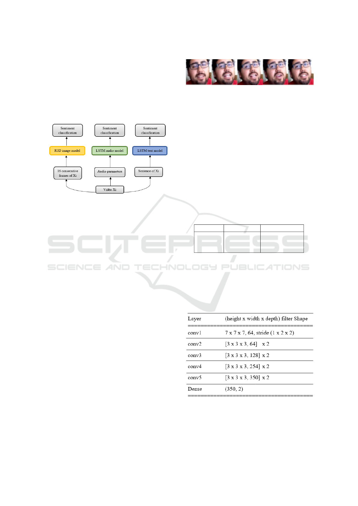
Figure 1 summarizes our unimodal pipeline ap-

proach. The three grey boxes at the bottom represent

the prepossessing of the data, the three colored boxes

are the deep learning models. In this approach, each

unimodal model predicts two class sentiment: posi-

tive or negative. The following subsections focus on

each modality.

Figure 1: Block diagram of our unimodal strategy.

3.1 Video Modality

Our approach privileges the 3D convolution on a

modiﬁed R3D model (Hara et al., 2017), designed

to reduce computation load. As a single frame con-

tains too few video features for sentiment classiﬁca-

tion, we decide to use neural networks with the abil-

ity to catch spatio-temporal features (change among

a given number of consecutive frames). The 3D-

CNN (C3D) (Tran et al., 2015) and Residual 3D-CNN

(R3D) (Hara et al., 2017), have been successfully ap-

plied in the past for action recognition. Due to em-

bedded constraints in computation and its outstand-

ing abilities in action recognition or classiﬁcation, we

prefer the R3D model. The general idea behind R3D

is to replace all two dimensional (2D) convolution in

the Resnet architecture (He et al., 2015) by 3D con-

volution. These two kind of models are fed with four

dimensional input deﬁned as R

f ∗c∗h∗w

where f is the

number of frames, c is the number of channels (three

i.e. for RGB images), h is the height of the frames

and w is the width of the frames.

Before feeding the network, we extract and crop

the head using key point detectors (Baltrusaitis et al.,

2018) instead of face detectors. With this approach,

we achieve precise alignment of the head between

each consecutive frame. We use the chin, ears, and

left and right eyebrows to determine a square and crop

it at this size. Next, the images are resized to 50px *

50px (see example Figure 2). This size is the best

compromise to obtain the best accuracy with the low-

est cost in computation. Indeed, there is a trade-off

Figure 2: Example of cropped face with 50 × 50 pixels.

between accuracy and the size of the input image in

CNN.

In the vein of previous sections, to reduce the

computational load, we also modify the last 3D con-

volution layers of the original R3D architecture. Less-

ening the numbers of ﬁlters from 512 to 350. This im-

provement reduces the numbers of parameters almost

by 13 million (see Table 2). This table shows that

the C3D model is not an adequate solution for em-

bedded systems. With equivalent performances, the

R3D model drastically reduces the number of param-

eters and the memory size of the model by a factor 2.

Finally, our R3D model reduces by factor 3 the num-

bers of parameters and the memory size by 2, which

represents a considerable improvement for equivalent

results.

Table 2: Comparison of three video-based CNN models.

Model #parameters Memory usage

C3D 63.32 M 300 MB

R3D 33.18 M 265 MB

our R3D 20.78 M 166 MB

Table 3 summarizes our model devoted to video.

The model takes in input 16 images. It is composed of

ﬁve 3D convolutional layers with an increasing num-

ber of ﬁlters on the low layers. Then the 350 extracted

features go through a dense layer to infer the ﬁnal pre-

diction.

Table 3: Our video-based CNN model.

3.2 Audio Modality

For the audio analysis, we experiment two techniques.

First, we experiment the classiﬁcation using Con-

VISAPP 2021 - 16th International Conference on Computer Vision Theory and Applications

390

volutional Neural Network (CNN). The objective is

to transform the signal into a spectral image (time-

frequency representation) and then feed the CNN with

it. This approach is widely used for sound and music

classiﬁcation (Hershey et al., 2017) or in emotional

and gender classiﬁcation (Arriaga et al., 2017).

The second model is a classiﬁcation using Long

Short Term Memory network (LSTM) (Hochreiter

and Schmidhuber, 1997). LSTM are a speciﬁc type of

Recurrent Neural Network (RNN). LSTM are today

mostly used to analyze sequential data. Its distinctive-

ness is the ability to memorize information during a

long period of time. To analyze our audio sequences,

we classically extract the audio features with openS-

MILE. We extract features every 100 ms with a slid-

ing window of 60 ms. We use Emobase2010, a con-

ﬁguration ﬁle for emotion classiﬁcation based on IN-

TERSPEECH 2010 para-linguistics (Schuller et al.,

2010). The default settings calculate 1582 features.

For time consuming purpose, we decrease to the ﬁrst

1054 features calculated by Emobase2010.

Table 4 illustrates our audio architecture. The

model is fed with a matrix of size ﬁxed: the width

is the numbers of features, and the height is the num-

bers of time step. Then the LSTM with two layers of

800 cells units each one, followed by a dense layer to

predict sentiments.

Table 4: Our audio-based LSTM models.

3.3 Text Modality

Concerning the text modality, we manually extract

the feature. We use the machine learning framework

scikit-learn. After creating a list with all words in

the dataset, we ﬁlter it to only keep adjectives and

verbs. Then each sentence is prepossessed to have

a ﬁxed length and be encoded into a number. Finally,

this vector goes through the embedding layer and then

feeds the LSTM.

Classically, LSTM text classiﬁers or generators

have an embedding layer to compress the input fea-

ture space into a smaller one. This embedding

layer (word2vec technique) is usually the Google

model trained on 100 billion words from Google

News (Mikolov et al., 2013). The weight of these lay-

ers cost more than 3.5 Go to load into memory. It

is not a feasible solution due to the constraint of the

hardware. Hence, we decide to train our own embed-

ding layer. Ultimately, the embedding layer uses a

text encoded vector of size 860 and generates a fea-

ture vector of size 100. Then, this vector feeds the

LSTM (see table 5) to ﬁnally predict sentiments. The

LSTM is structured with two layers of 32 cells units

each one, followed with a dense layer for the ﬁnal

prediction.

Table 5: Our text-based LSTM model.

3.4 Multimodal Fusion

Figure 3 illustrates our multimodal late fusion strat-

egy. The three grey squares on the bottom repre-

sent the prepossessing of the data, the three colored

squares are the deep learning models. For the fusion,

the models are modiﬁed to be combined in the orange

box. A ﬁnal model predicts the positive vs. negative

sentiment.

We consider two fusion strategies, one based on

mathematical model with the theory of evidence and

one based on data driven with a dense network layer.

The evidence theory is well adapt to model the relia-

bility of different channels. We choose to implement

it instead of SVM or Bayesian theory because they

only concern a single evidence and they cannot de-

scribe the probability of ignorance. In addition, the

SVM classiﬁer shows the lowest results for such ap-

plication (see (Cambria et al., 2017)). For the data

driven fusion, we choose the trainable technique that

requires the least amount of computing resources (i.e

the fully connected layer that is the most basic neural

network layer).

3.4.1 Fusion with Theory of Evidence (Dempster

Shafer)

Dempster-Shafer Theory (DST) (Shafer, 1976) com-

bines evidence of information from multiple events to

calculate the belief of the occurrence of another event.

Let Θ =

{

, X

, ..., X

}

be a ﬁnite set called a frame

of discernment. 2

refers to every possible mutually

exclusive subset of the elements of Θ.

Multimodal Neural Network for Sentiment Analysis in Embedded Systems

391

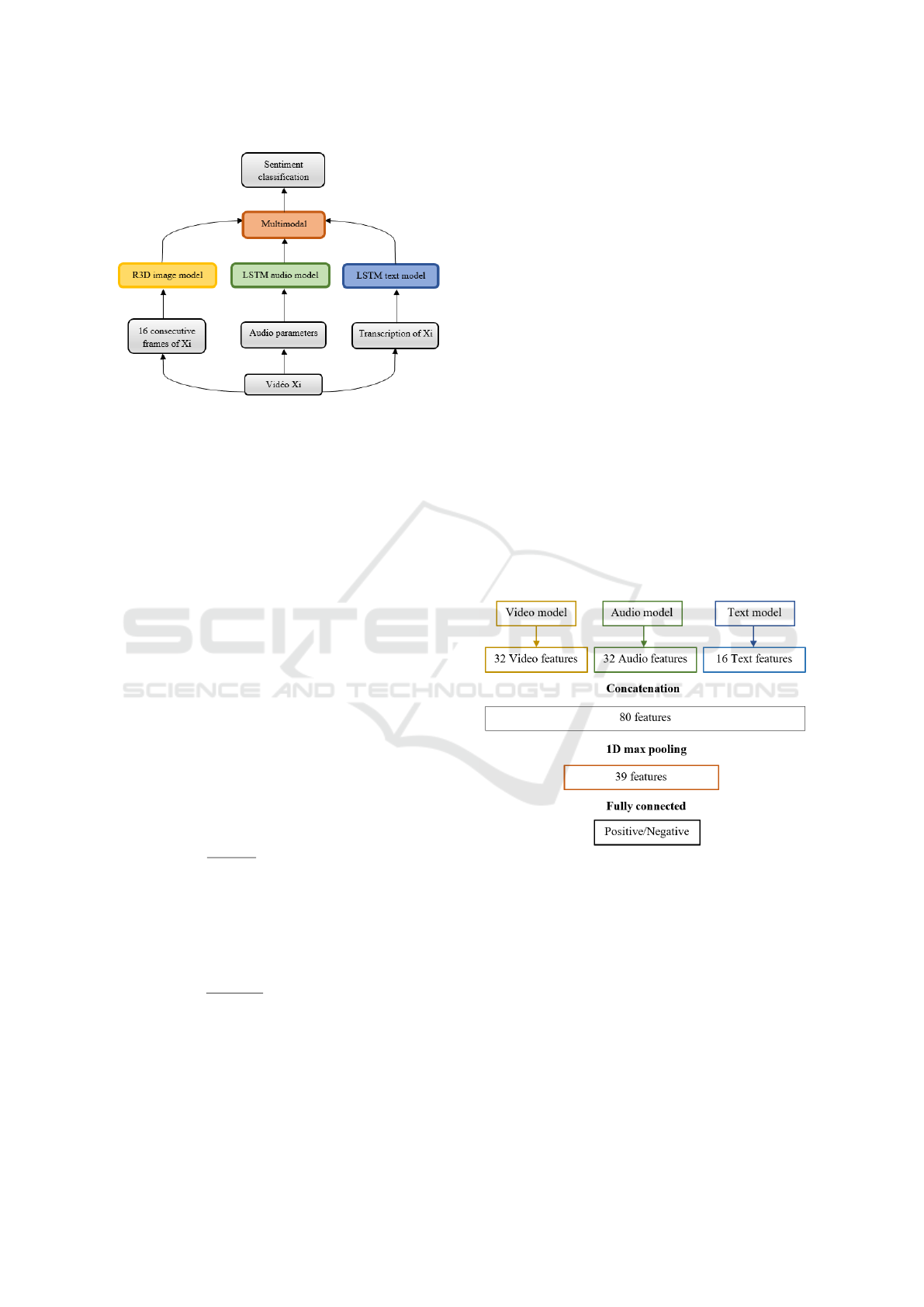
Figure 3: Block diagram of our complete multimodal sys-

tem.

Each subset receives a belief value within [0, 1].

In this approach, the uncertainty is estimated based

on the recall metric.

The mass probability, denoted m(X), is used to as-

sign evidence to a given modality X.

Where:

0 ≤ m(X

) ≤ 1,

∑

X⊆Θ

m(X) = 1, m(

0) = 0 (2)

In our framework, we have three mass probabil-

ities m

(X), m

(X), one for each modality.

Each model outputs a number of probabilities equal

to the numbers of labels. We also calculate the recall

performances of each model. The recall measures the

percentage of positive samples correctly classiﬁed.

With all these elements we can compute the DST

fusion.

Video/Text joint mass:

V,T

∑

∩X

) × m

) (3)

V T

(Z) =

1 − k

V,T

∑

Xi∩X j=Z

(Xi)m

) (4)

Video/Text/Audio joint mass:

V T,A

∑

∩X

V T

) × m

) (5)

V T,A

(Z) =

1 − k

V T,A

∑

∩X

V T

) × m

(X j)

(6)

With X

= Negative, X

= Positive

V T,A

(Z) is a table of size 3. The ﬁrst 2 columns

are the probabilities of the negative and positive class.

The last column is the uncertainty. To calculate the ﬁ-

nal F1

score

, we take the index of the maximum value

of the ﬁrst 2 columns. The index return the predic-

tion of the label (i.e 0 or 1). Then the ﬁnal F1

score

calculated using the prediction and the ground-truth.

This fusion strategy does not require any addi-

tional training and it is computationally cheap to em-

bed. However, the drawback is that time consuming

increases with the number of possible of modality to

fuse.

3.4.2 Features Level Fusion using Fully

Connected Layer (FC)

For this fusion approach, we use a late fusion. It al-

lows to use different models on each modality. It

is more ﬂexible than early fusion. To combine our

three unimodal models, we modify the output of each

model to ﬁnally have 32 features for audio and video

(respectively yellow and green on the Figure 4) and

16 features for text (in blue on Figure 4). At this

time, we applied a concatenation to obtain a vector of

80 features. These numbers of features were chosen

empirically, we noticed that more the model is con-

strained with a few numbers of parameters better are

the results. Indeed, the network tries to ﬁnd out which

parameters are the most valuable.

Figure 4: Feature concatenation for FC fusion purpose.

Then, a 1D max pooling layer is applied to get

the 39 most important features of the input. The max

pooling operation consist to downsamples the input

by taking the maximum value over a window of size

ﬁxed. Then the window is shifted across the input.

At this time, a fully connected layer of 78 parameters

is applied to get the ﬁnal sentiment prediction. With

only 78 parameters the impact on the embedded per-

formances are very low.

VISAPP 2021 - 16th International Conference on Computer Vision Theory and Applications

392

4 IMPLEMENTATION

This section details ﬁrst the MOSI dataset. Then we

present the improvement made on the pre-processing

phase to reduce embedded performances. Finally,

we present the implementation of the training phase.

During all the experiments, we use the F1 score as

evaluation metric.

The F1 score is deﬁned as follows:

score

= 2 ∗

Recall ∗ Precision

Recall + Precision

(7)

4.1 Dataset MOSI

The MOSI dataset contains 93 videos recorded thanks

to 89 different speakers. It is divided and annotated

into 2199 sub-sequences (utterances). The topic of

the dataset is English reviews on movies or books (see

Table 6 for full details of the dataset). A key point

when we work on sentiment analysis, is the speaker

dependency. The idea is to evaluate the abilities of the

algorithm to generalize when it sees a new speaker.

In order to compare the performances with the liter-

ature we split the dataset like (Cambria et al., 2017)

and (Poria et al., 2017). The ﬁrst 62 videos (≈ 70%)

of the dataset are used for train/validation and the re-

maining ones (≈ 30%) are used for the test phase.

Table 6: Details of the MOSI dataset.

Train Test

Nbrs of videos 62 31

Utterances 1447 752

Nbrs of speaker 58 31

Man 33 15

Woman 25 16

Video/Audio (min) ≈ 85 ≈ 50

Sentences 1447 752

Nbrs of word 17296 9161

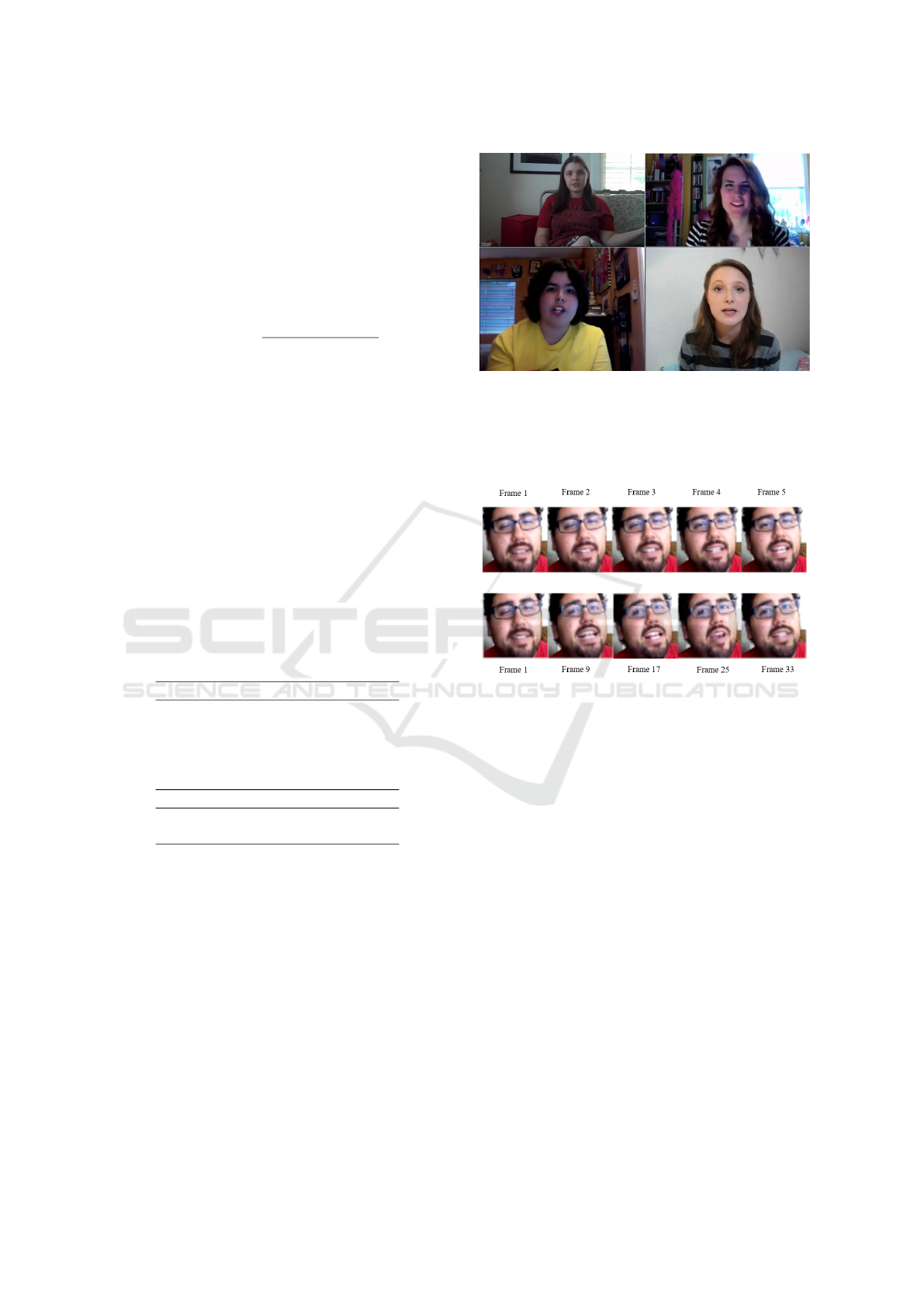
A key point for us is the relative position between

the scene and the camera. He has to be recorded in

front of their camera. Face frontal view are recorded

(i.e similar to Vlog format) in the vein of MOSI (see

ﬁgure 5). Our ﬁnal context is an in-vehicle situation,

where drivers will be analyzed with a front view cam-

era.

4.2 Computation Considerations

We implement some basic improvement in the pre-

processing phase to reduce computational resources.

On the video ﬁle, particularly in the MOSI dataset,

consecutive video frames represent redundant infor-

mation. To overcome this problem, we downscale the

Figure 5: Front view examples of MOSI dataset.

frame rate of the video. In our experiment we reduce

it by a factor 4, 8, 16, 32. The most outstanding per-

formances are for the factor 8. We can see the differ-

ence between a factor 1 and 8 on Figure 6.

Figure 6: Examples of downscaling frame rate. The ﬁrst

row represents a video with successive frames. The second

row shows the same video downsized with a factor 8.

On the audio analysis we test two models in order

to reduce computation. For the ﬁrst model, we avoid

the dependency to a speciﬁc feature’s extractor. So,

we use a 2D CNN as a features extractor followed by

a dense layer for the classiﬁcation. The results are

not signiﬁcant in our case. With the second approach,

we use OpenSMILE as a feature extractor and then

we use an LSTM model followed by a dense layer for

the classiﬁcation. By reducing the input matrix of the

LSTM we can reduce the computation. After trials

and errors, we reduce the width of the input matrix to

only 1054 features.

The text data is the transcription of spoken sen-

tences. All the sentences represent a total of 26,457

words and 3003 unique words. To improve embedded

performances, we ﬁlter all the words. After a few ex-

periments, we only kept adjectives and adverbs. This

conﬁguration provides the most signiﬁcant rate of ac-

curacy vs. numbers of words. The ﬁltering approach

reduces the numbers of words to 860. At this point,

we calculate the frequency distribution. Finally, the

Multimodal Neural Network for Sentiment Analysis in Embedded Systems

393

length of sentences is wrapped to a window of 30

words. After a few experiments, we determine that

this length leads to the best results.

The reader can refer to the table 7 where the 10

most important and less important words are listed.

Table 7: Frequency of words in the dataset.

10 most present 10 less present

words

really catastrophic

good mid

whole oldest

i rough

little meanwhile

not papa

pretty guys

sad overly

awesome upbeat

funny relatable

4.3 Implementation Details

Unlike (Poria et al., 2017), we do not consider the

inter-utterance level. An utterance is a continuous

unit of speech beginning and ending with an explicit

pause. We consider in our approach that when we

classify one utterance, others utterances do not con-

vey more contextual information. We merely predict

the three modalities of one utterance. This approach

permits to only use 2 LSTM models in the ﬁnal archi-

tecture.

4.3.1 Transfer Learning

To train the multimodal model, we use transfer learn-

ing (see (Pan and Yang, 2010) for a comprehensive

review). Indeed, instead of starting the learning pro-

cess from scratch, we start from a model that has been

learning how to solve diverse problems. This tech-

nique drastically reduces the training time. Transfer

learning includes two different approaches: develop-

ing models and pre-training. It is a widely used ap-

proach in deep learning (He et al., 2015; Krizhevsky

et al., 2012; Rawat and Wang, 2017). We implement

pre-training. It consists in selecting a source model,

then in reusing it from a starting point, and ﬁnally to

tune the model for our task. We use the unimodal

model at their best accuracy point to train the ﬁnal

multimodal model.

In our case, the use of pre-training techniques is

necessary. Indeed, the fully connected fusion model

would not be able to converge if we start the training

from scratch. The FC layer includes only 78 hyper

parameters (randomly initialized) which constraints

the network. By this layer, we force it to pro-

duce its proper decisions.

4.3.2 Tuning of Hyper Parameters

Every training of each model is performed using the

categorical cross-entropy loss. For the MOSI dataset

the literature predicts two classes. For Binary classi-

ﬁcation the formula of cross-entropy loss becomes:

loss = −(ylog(p) + (1 − y) log(1 − p))

With p the prediction of the network and y the associ-

ated ground truth.

We consider two different optimizers: stochastic

descent gradient to train the video model and Adam

optimizer (Kingma and Ba, 2017) for audio and text

model. Indeed, empirically we found that Adam is

more skillful to train networks with sparse input data

which is claimed by (Kingma and Ba, 2017).

Concerning the regularization, we use dropout di-

rectly in the audio and text LSTM model to reduce

the variance. A dropout of 0.4 (resp. 0.6) is applied

on the audio (resp. text).

Learning rate is precisely chosen for each modal-

ity and the fully connected fusion model. To train the

unimodal model, the learning rate is set at 10

−3

−5

. As we use the unimodal pre-trained model to

train the fully connected multimodal model, we re-

duce the learning rate. By default, the learning rate

starts from 10

−4

to 10

−6

, while the learning rate of

FC is multiplied by ten times the default learning rate.

5 EVALUATION AND

ASSOCIATED ANALYSIS

First, this section presents the evaluations and com-

pare them with the state of the art approach. Second,

we propose a qualitative analysis illustrated by some

results.

5.1 Quantitative Evaluations

As we can see in the table 8, each modality does not

carry the same amount of information. Video is in-

efﬁcient with an F1 score of 57%, close to random

prediction. The audio modality arrives in second po-

sition with an F1 score of 65.5%. Ultimately, text has

the best F1 score with 77.1%. Our fusion results are

78% for DST fusion and 80% for FC fusion, showing

respectively an improvement of 1% and 3% compared

to unimodal approaches. The FC fusion obtains the

most outstanding results and the 78 parameters are in-

signiﬁcant with regard to the embedded performance

(i.e. increase in memory load and computing).

VISAPP 2021 - 16th International Conference on Computer Vision Theory and Applications

394

Contrarily to (Poria et al., 2017), we improve

the performances of the audio and video classiﬁca-

tions (gains of 1.4% and 5.2% respectively). Our text

model performs 1% worse. This 1% performance re-

duction is due to the fact that we use our own embed-

ding layers trained on MOSI instead of the Google

embedding layers. The performances of the FC fusion

model is 0.3% under (Poria et al., 2017) approach.

Our framework, similarly to the most of existing

approaches evaluated on the MOSI dataset, shows the

same order of modality importance (video is not much

informative, audio and text are a little and very infor-

mative) (see (Poria et al., 2017; Cambria et al., 2017;

Huddar et al., 2018))

Table 8: Comparison of the proposed variants. The table

reports the F1 score.

Modality Source F1 score

Unimodal

Video 0.572

Audio 0.655

Text 0.771

Unimodal

(Poria et al.,

2017)

Video 0.558

Audio 0.603

Text 0.781

DST fusion Video + Audio + Text 0.780

FC fusion Video + Audio + Text 0.800

bc-LSTM

(Poria et al.,

2017)

Video + Audio + Text 0.803

Contrasting the embedded performances with the

ones in the literature is extremely complex because

they do not consider the embedded performances.

They exclusively focus on accuracy. We can certainly

compare our work with (Poria et al., 2017):

• video: we reduce by 3 the numbers of parameters

and by 2 the memory usage.

• audio: we reduce by 6 the number of audio fea-

tures feeding the LSTM model.

• text: we reduce by 3.5Go the memory use of the

model.

• fusion: our fusion approach includes only 78 pa-

rameters instead of a bi-directional LSTM com-

posed of 600 units cells.

• They use three bi-directional LSTM after each

modality to catch contextual information inter-

utterances which add 1800 units cells. Our ap-

proach does not possess it.

Overall, compared to the reference approach on

MOSI, we reduce by 2.2 the numbers of parameters

and the memory usage by 13.8.

Presently, if we compare the performances of ac-

curacy vs. embedded capability performances, we

can notice that text modality is crucial on the MOSI

dataset. The transcription brings 77% of the informa-

tion with only 112k parameters and 1.3MB of mem-

ory (see table 9).

Table 9: Computational resources of all variants.

Model Parameters Memory load

R3D 20.78 M 166 MB

LSTM audio 11.25 M 133.5 MB

LSTM text 112 k 1.3 MB

DST fusion 32.14 M 300.8 MB

FC fusion 32.14 M + 78 300.8 MB

bc-LSTM

(Poria et al.,

2017)

≈ 70 M ≈ 4.15 Go

As expected, our approach leads to state-of-art

performances while reducing drastically computation

and memory size.

5.2 Qualitative Evaluations

We recover all misclassiﬁed ﬁles for each modality in

order to achieve a more proper understanding of our

approach. The limit with the MOSI dataset is the fact

that the subject can express sentiments in total con-

tradiction of the movie sentiment. It is challenging

for the model to differentiate the speaker’s sentiments

from the movie’s sentiment. For instance, the subject

tells calmly: ”I love the war scene”. And it would

be classiﬁed as negative by the audio and text model.

But the ground truth is positive. At this moment, the

sentiment of the speaker is positive with the sentiment

”love” but the sentiment expressed by the context of

the ﬁlm can be interpreted as negative with the word

”war.” This kind of issue represents 15% of the mis-

classiﬁed samples.

As expected, there are many video ﬁles misclas-

siﬁed. This is most likely due to the fact that people

are making reviews in front of the camera without hu-

man interactions. Sometimes the length of the audio

or the text ﬁle is extremely short. The audio can also

contains very prolonged pause and the text contains

not enough words. Those two factors are responsible

for a lack of context especially for architecture like

LSTM, inducing a misclassiﬁcation. Some examples

of poor sentences: ”and it would make sense” or ”I

wish I weren’t.”. These types of problems represents

45% of the misclassiﬁed samples.

Another limitation is that some audio recordings

are absolutely neutral and the words contained in the

sentences do not provide enough meaning to classify

Multimodal Neural Network for Sentiment Analysis in Embedded Systems

395

correctly. Some examples of sentences without mean-

ing could be: ”I would like to quickly talk about Ma-

chete.” This category of error represents 35% of the

misclassiﬁed samples.

Finally, the latter limit identiﬁed in this dataset is

the quality of the recording which can impact the clas-

siﬁcation. This, represents 5% of misclassiﬁed sam-

ples. Several of them have extremely poor video qual-

ity and critical audio quality with some noises due to

the old webcams used for the records.

6 CONCLUSION AND FUTURE

WORKS

The embeddability capability of CNN networks is of-

ten omitted in the literature and even more in multi-

modal systems where models tend to be computation-

ally expensive. Our developed model leads to perfor-

mances similar to the literature but with a high em-

beddable capability i.e reducing by 2.2 (resp. 13.8)

the numbers of parameters (resp. the memory load).

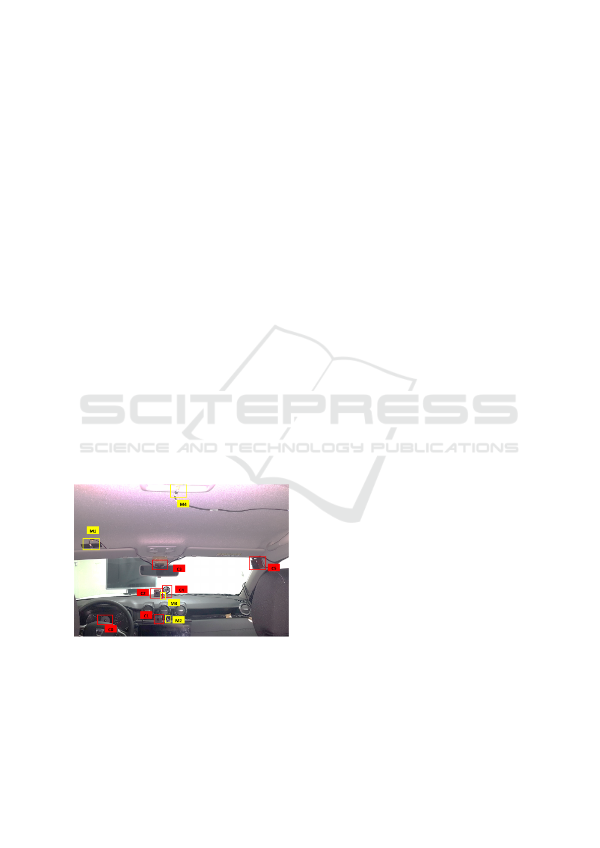
We are actually working with a real context

dataset which is composed of one driver and one pas-

senger (sat in the back). The subjects are put in dif-

ferent social situations without following scripts. Six

cameras and four microphones set at different posi-

tions in the car are installed. Figure 7 shows the

recording setup. Future works could use and adapt

our model training to such a vehicle context dataset,

with the objective to analyze sentiment interactions

between two passengers.

Figure 7: Recording setup of the Renault dataset. Red

squares refer to the cameras numbered from C0 to C5. Yel-

low squares refer to microphone numbered from M1 to M4.

Moreover, as humans are not varying their emo-

tions every seconds, an interesting approach is to

use based model theories (decision three or Hidden

Markov) or a deep learning model as an output of the

actual framework. These techniques could be promis-

ing in order to keep track of the sentiments or the

emotions of both the driver and the passenger.

ACKNOWLEDGEMENT

This work has been carried out under the funding

of an industrial doctorates fellowship from National

Association for Research and Technology (ANRT),

France.

REFERENCES

Agarwal, A., Yadav, A., and Vishwakarma, D. K. (2019).

Multimodal sentiment analysis via rnn variants. In

2019 IEEE International Conference on Big Data,

Cloud Computing, Data Science Engineering (BCD),

pages 19–23.

Arriaga, O., Valdenegro-Toro, M., and Pl

oger, P. (2017).

Real-time convolutional neural networks for emotion

and gender classiﬁcation. arXiv:1710.07557 [cs].

Baltrusaitis, T., Zadeh, A., Lim, Y. C., and Morency,

L. (2018). Openface 2.0: Facial behavior analysis

toolkit. In 2018 13th IEEE International Conference

on Automatic Face Gesture Recognition (FG 2018),

pages 59–66.

Baqeel, H. and Saeed, S. (2019). Face detection authentica-

tion on smartphones: End users usability assessment

experiences. In 2019 International Conference on

Computer and Information Sciences (ICCIS), pages

1–6.

Benedetto, F. and Tedeschi, A. (2016). Big data sentiment

analysis for brand monitoring in social media streams

by cloud computing. In Pedrycz, W. and Chen, S.-M.,

editors, Sentiment Analysis and Ontology Engineer-

ing: An Environment of Computational Intelligence,

pages 341–377. Springer International Publishing.

Bochkovskiy, A., Wang, C.-Y., and Liao, H.-Y. M. (2020).

YOLOv4: Optimal speed and accuracy of object de-

tection. arXiv:2004.10934 [cs, eess].

Busso, C., Bulut, M., Lee, C.-C., Kazemzadeh, A., Mower,

E., Kim, S., Chang, J. N., Lee, S., and Narayanan,

S. S. (2008). IEMOCAP: interactive emotional dyadic

motion capture database. Language Resources and

Evaluation, 42(4):335–359.

Cambria, E., Hazarika, D., Poria, S., Hussain, A., and Sub-

ramaanyam, R. B. V. (2017). Benchmarking multi-

modal sentiment analysis. arXiv:1707.09538 [cs].

Carroll, J. B. (1938). Diversity of vocabulary and the har-

monic series law of word-frequency distribution. The

Psychological Record, 2(16):379–386.

Cerutti, G., Prasad, R., and Farella, E. (2019). Convolu-

tional neural network on embedded platform for peo-

ple presence detection in low resolution thermal im-

ages. In ICASSP 2019 - 2019 IEEE International Con-

VISAPP 2021 - 16th International Conference on Computer Vision Theory and Applications

396

ference on Acoustics, Speech and Signal Processing

(ICASSP), pages 7610–7614.

Dubey, A. R., Shukla, N., and Kumar, D. (2020). Detec-

tion and classiﬁcation of road signs using HOG-SVM

method. In Elc¸i, A., Sa, P. K., Modi, C. N., Olague,

G., Sahoo, M. N., and Bakshi, S., editors, Smart Com-

puting Paradigms: New Progresses and Challenges,

pages 49–56. Springer Singapore.

Eyben, F., W

ollmer, M., and Schuller, B. (2010). opensmile

– the munich versatile and fast open-source audio fea-

ture extractor. In ACM Multimedia, pages 1459–1462.

Feng, W., Guan, N., Li, Y., Zhang, X., and Luo, Z. (2017).

Audio visual speech recognition with multimodal re-

current neural networks. In 2017 International Joint

Conference on Neural Networks (IJCNN), pages 681–

688. ISSN: 2161-4407.

Greco, F. and Polli, A. (2020). Emotional text mining: Cus-

tomer proﬁling in brand management. International

Journal of Information Management, 51:101934.

Hara, K., Kataoka, H., and Satoh, Y. (2017). Learning

spatio-temporal features with 3d residual networks for

action recognition. arXiv:1708.07632 [cs].

He, K., Zhang, X., Ren, S., and Sun, J. (2015). Deep resid-

ual learning for image recognition. arXiv:1512.03385

[cs].

Hershey, S., Chaudhuri, S., Ellis, D. P. W., Gemmeke,

J. F., Jansen, A., Moore, R. C., Plakal, M., Platt,

D., Saurous, R. A., Seybold, B., Slaney, M., Weiss,

R. J., and Wilson, K. (2017). CNN architectures

for large-scale audio classiﬁcation. arXiv:1609.09430

[cs, stat].

Hochreiter, S. and Schmidhuber, J. (1997). Long short-term

memory. Neural computation, 9:1735–80.

Howard, A., Sandler, M., Chu, G., Chen, L.-C., Chen, B.,

Tan, M., Wang, W., Zhu, Y., Pang, R., Vasudevan, V.,

Le, Q. V., and Adam, H. (2019). Searching for mo-

bilenetv3.

Huddar, M. G., Sannakki, S. S., and Rajpurohit, V. S.

(2018). An ensemble approach to utterance level mul-

timodal sentiment analysis. In 2018 International

Conference on Computational Techniques, Electron-

ics and Mechanical Systems (CTEMS), pages 145–

150.

Kahou, S. E., Bouthillier, X., Lamblin, P., Gulcehre,

C., Michalski, V., Konda, K., Jean, S., Frou-

menty, P., Dauphin, Y., Boulanger-Lewandowski, N.,

Chandias Ferrari, R., Mirza, M., Warde-Farley, D.,

Courville, A., Vincent, P., Memisevic, R., Pal, C.,

and Bengio, Y. (2016). EmoNets: Multimodal deep

learning approaches for emotion recognition in video.

Journal on Multimodal User Interfaces, 10(2):99–

111.

Kingma, D. P. and Ba, J. (2017). Adam: A method for

stochastic optimization. arXiv:1412.6980 [cs].

Krizhevsky, A., Sutskever, I., and Hinton, G. E. (2012). Im-

ageNet classiﬁcation with deep convolutional neural

networks. In Pereira, F., Burges, C. J. C., Bottou,

L., and Weinberger, K. Q., editors, Advances in Neu-

ral Information Processing Systems 25, pages 1097–

1105. Curran Associates, Inc.

Li, H., Sun, J., Xu, Z., and Chen, L. (2017). Multimodal

2d+3d facial expression recognition with deep fusion

convolutional neural network. IEEE Transactions on

Multimedia, 19(12):2816–2831. Conference Name:

IEEE Transactions on Multimedia.

Maas, A. L., Daly, R. E., Pham, P. T., Huang, D., Ng, A. Y.,

and Potts, C. (2011). Learning word vectors for sen-

timent analysis. In Proceedings of the 49th Annual

Meeting of the Association for Computational Lin-

guistics: Human Language Technologies, pages 142–

150, Portland, Oregon, USA. Association for Compu-

tational Linguistics.

Mao, J., Xu, W., Yang, Y., Wang, J., Huang, Z., and Yuille,

A. (2015). Deep captioning with multimodal recurrent

neural networks (m-RNN). arXiv:1412.6632 [cs].

Mikolov, T., Chen, K., Corrado, G., and Dean, J. (2013).

Efﬁcient estimation of word representations in vector

space.

antyl

a, M. V., Graziotin, D., and Kuutila, M. (2018). The

evolution of sentiment analysis—a review of research

topics, venues, and top cited papers. Computer Sci-

ence Review, 27:16 – 32.

Morency, L.-P., Mihalcea, R., and Doshi, P. (2011). To-

wards Multimodal Sentiment Analysis: Harvesting

Opinions from The Web. In International Confer-

ence on Multimodal Interfaces (ICMI 2011), Alicante,

Spain.

Nandal, N., Tanwar, R., and Pruthi, J. (2020). Machine

learning based aspect level sentiment analysis for

amazon products. Spatial Information Research.

Pan, S. J. and Yang, Q. (2010). A survey on transfer learn-

ing. IEEE Transactions on Knowledge and Data En-

gineering, 22(10):1345–1359.

erez-Rosas, V., Mihalcea, R., and Morency, L.-P. (2013).

Utterance-level multimodal sentiment analysis. In

Proceedings of the 51st Annual Meeting of the Associ-

ation for Computational Linguistics (Volume 1: Long

Papers), pages 973–982, Soﬁa, Bulgaria. Association

for Computational Linguistics.

Poria, S., Cambria, E., Hazarika, D., Majumder, N., Zadeh,

A., and Morency, L.-P. (2017). Context-dependent

sentiment analysis in user-generated videos. In Pro-

ceedings of the 55th Annual Meeting of the Associa-

tion for Computational Linguistics (Volume 1: Long

Papers), pages 873–883. Association for Computa-

tional Linguistics.

Pradeep, K., Kamalavasan, K., Natheesan, R., and Pasqual,

A. (2018). Edgenet: Squeezenet like convolution neu-

ral network on embedded fpga. In 2018 25th IEEE

International Conference on Electronics, Circuits and

Systems (ICECS), pages 81–84.

Rawat, W. and Wang, Z. (2017). Deep convolutional neural

networks for image classiﬁcation: A comprehensive

review. Neural Computation, 29:1–98.

Reshma, B. and Kiran, K. A. (2017). Active noise cancel-

lation for in-ear headphones implemented on fpga. In

2017 International Conference on Intelligent Comput-

ing and Control Systems (ICICCS), pages 602–606.

Schuller, B., Steidl, S., Batliner, A., Burkhardt, F., Dev-

illers, L., Muller, C., and Narayanan, S. S. (2010). The

Multimodal Neural Network for Sentiment Analysis in Embedded Systems

397

INTERSPEECH 2010 paralinguistic challenge. IN-

TERSPEECH 2010, page 4.

Shafer, G. (1976). A Mathematical Theory of Evi-

dence. Princeton University Press. Google-Books-ID:

wug9DwAAQBAJ.

Shi, J., Zhang, G., Yuan, J., and Zhang, Y. (2020). Im-

proved YOLOv3 infrared image pedestrian detection

algorithm. In Zeng, J., Jing, W., Song, X., and Lu, Z.,

editors, Data Science, pages 506–517. Springer Sin-

gapore.

Tran, D., Bourdev, L., Fergus, R., Torresani, L., and Paluri,

M. (2015). Learning spatiotemporal features with 3d

convolutional networks. In The IEEE International

Conference on Computer Vision (ICCV).

Trupthi, M., Pabboju, S., and Narasimha, G. (2017). Senti-

ment analysis on twitter using streaming api. In 2017

IEEE 7th International Advance Computing Confer-

ence (IACC), pages 915–919.

Vu, T., Nguyen, C. V., Pham, T. X., Luu, T. M., and Yoo,

C. D. (2019). Fast and efﬁcient image quality en-

hancement via desubpixel convolutional neural net-

works. In Leal-Taix

e, L. and Roth, S., editors, Com-

puter Vision – ECCV 2018 Workshops, volume 11133,

pages 243–259. Springer International Publishing. Se-

ries Title: Lecture Notes in Computer Science.

ollmer, M., Weninger, F., Knaup, T., Schuller, B., Sun,

C., Sagae, K., and Morency, L. (2013). Youtube

movie reviews: Sentiment analysis in an audio-visual

context. IEEE Intelligent Systems, 28(3):46–53.

orle, J., Metz, B., Othersen, I., and Baumann, M. (2020).

Sleep in highly automated driving: Takeover perfor-

mance after waking up. Accident Analysis & Preven-

tion, 144:105617.

Zadeh, A., Zellers, R., Pincus, E., and Morency, L.-P.

(2016). Mosi: Multimodal corpus of sentiment inten-

sity and subjectivity analysis in online opinion videos.

Zhao, H., Zhang, W., Sun, H., and Xue, B. (2019). Embed-

ded deep learning for ship detection and recognition.

Future Internet, 11(2):53.

VISAPP 2021 - 16th International Conference on Computer Vision Theory and Applications

398