Decision Support for Bundle Shipment Choices: Orthogonal

Two-dimensional Bin Packing with Practical Constraints

Yizi Zhou

, Jiyin Liu

, Rupal Mandania

, Shuyang Li

, Kai Chen

and Rongjun Xu

Huawei Technologies Co Ltd, Bantian Huawei Base, Shenzhen, China

School of Business and Economics, Loughborough University, Loughborough, U.K.

Keywords: Orthogonal 2D-BPP, LTL Shipping, FTL Shipping, Mixed-integer Linear Programming.

Abstract: In this paper, we study a real life application of an orthogonal two dimensional bin packing problem (2D-

BPP) with a small assortment of different shapes of bins and items. A telecommunication equipment company

ships its products to customers several times daily by trucks and it currently uses the less-than-truckload

(LTL) shipping option which is priced as unit price per volume times the total volume of products. However,

depending on scale of products to be shipped, full-truckload (FTL) shipping which is priced as a single price

per truck may be cheaper. In this paper we aim to help the company to decide on the delivery choice as well

as on how to pack the truck optimally when FTL shipping is selected. We model the problem as a variant of

an orthogonal 2D-BPP using mixed-integer linear programming (MIP) with the objective to minimise the

total cost of delivery. Practical conditions influencing the feasibility of packing patterns are also considered.

Practical guidance such as those on some modelling techniques and the application of the model, are applied

to enhance the solving efficiency. The problems are solved by commercial solver CPLEX to optimality up to

34 pallets within an acceptable time. For lager problems, we adopt an approach to combine same items into

larger rectangles and then pack them. This increases the solvability to 154 pallets. On average, our method

help the company save 26% shipping cost.

1 INTRODUCTION

We study a problem where a telecommunication

equipment company sends products from warehouses

to customer sites in mainland China once a day by

truck. There are two types of truck delivery service:

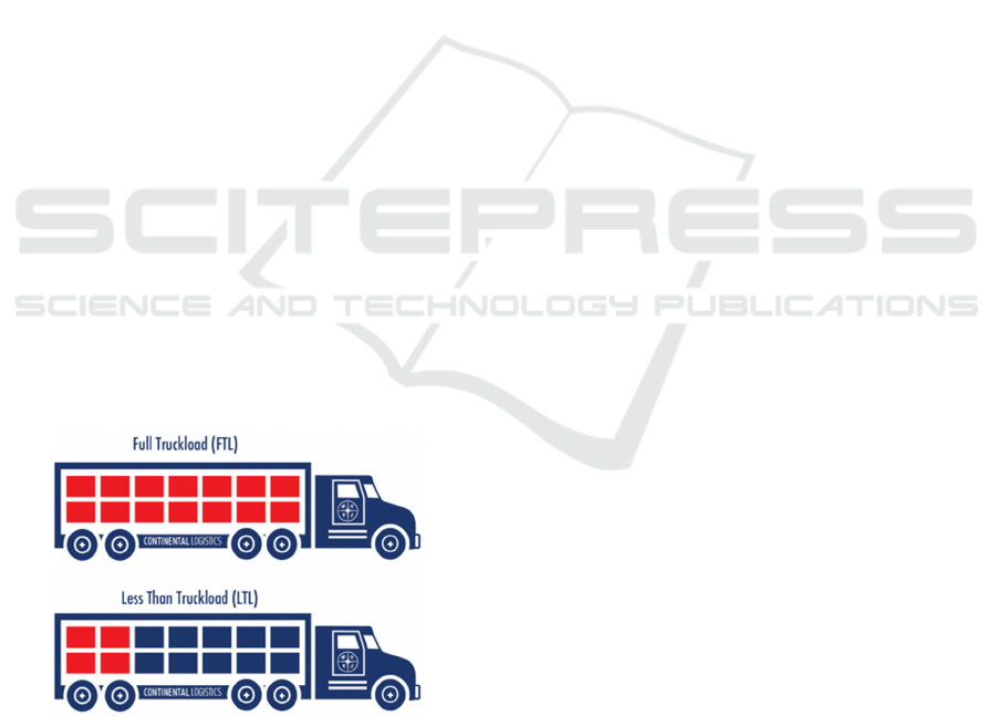
less-than-truckload (LTL) shipping and full-

truckload (FTL) shipping, as illustrated in Figure 1.

LTL is priced as unit price multiplied by total volume

of products shipped and normally the products are

packed with products of other companies. FTL is

priced as a single price per truck. When there is a

small amount of products, it is cheaper to use LTL

shipping. However, when there is a large amount of

products, the company should choose FTL shipping.

The service level agreement (SLA) of FTL is also

faster than FTL. For FTL shipping, the company need

to load the products themselves. This part of cost is

internal and negligible. The decisions to make are on

https://orcid.org/0000-0003-2140-9801

https://orcid.org/0000-0002-2752-5398

https://orcid.org/0000-0002-9025-0569

the type of shipping to choose, the number of trucks

needed for FTL and the loading sequence and

positions of products onto each truck. We modelled

the problem as a variant of an orthogonal 2D-BPP

using mixed-integer linear programming (MIP) with

the objective to minimise the total cost of delivery. It

combines two discrete optimization problems: Bin

packing and optimal bundle shipment decisions. It is

therefore modelled as an integrated mixed integer

programing model (MIP) with two sets of constraints:

one for bin packing and the other for bundle shipment

cost computation. The products to be packed are

fragile and cannot be stacked, which means there is

only one layer of products inside a truck. Practical

constraints are also needed, for example, no more

than two customers can be loaded onto the same

truck, some customers must be delivered later on the

route as the unloading time could be long for those

customers due to warehouse service capability, and

Zhou, Y., Liu, J., Mandania, R., Li, S., Chen, K. and Xu, R.

Decision Support for Bundle Shipment Choices: Orthogonal Two-dimensional Bin Packing with Practical Constraints.

DOI: 10.5220/0010221201610168

In Proceedings of the 10th International Conference on Operations Research and Enterprise Systems (ICORES 2021), pages 161-168

ISBN: 978-989-758-485-5

161

products for the same customers must be placed

together for unloading convenience. We solve the

problems using CPLEX solver. Experiments are

carried out to demonstrate the performance of the new

model. A 26% of reduction in delivery cost is

achieved by applying this model in real life cases.

Also, we provide some practical guidance on how to

reformulate the problem with care to improve the

solving efficiency. We solve the reformulated model

on the same numerical examples and reduced the

computational time to 1/100% of before which helps

the model to be implemented in real life business.

The paper is organized as follows. In section 2,

literature on the 2D-BPP formulation, typology,

practical applications, and related solution algorithms

are reviewed. Section 3 presents the mathematical

models for our problem and discusses how to pick up

an appropriate value for the number of trucks to be

used in the model when infinitely many are available.

In section 4, the proposed mathematical model is

tested through numerical experiments using general

purpose MIP solver. A 26% saving in delivery cost is

achieved on real life instances with this model. In

section 5, we discuss how to improve the solving

efficiency by choosing fixed charges in the MIP

formulation, reducing symmetry and carefully

implementing the MIP model for large cases. We

show how careful formulation for a mixed integer

program (MIP) can lead to a solution of the

mathematical model in a reasonable amount of time,

while some formulations of the same problem can

make the model practically unsolvable. The reduction

in computational time is critical for practical

implementation. Finally, conclusions and future

research directions are provided in section 6.

Figure 1: Illustration of FTL Shipping vs. LTL Shipping.

2 LITERATURE REVIEW

The basic BPP involves two sets, one set of bins, with

same size or different sizes, and one set of items to be

packed normally with different sizes. All items and

bins have fixed rectangular shapes. The problem is to

place the items within the bins in order to optimize

some functions, such as minimise the bins used,

minimise cost, or maximise the items packed, subject

to some physical or business constraints. Commonly

considered physical constraints are: items cannot

overlap (share the same region in the truck) if they are

assigned to the same truck and any item must be

completely located within a bin. The number of

dimensions involved define the problem into 2D and

3D BPP referring to two-dimensional and three-

dimensional problems. As the pallets contains

valuable objects that cannot be stacked so we simplify

the problem into 2D-BPP and are only interested in

the arrangement of the pallets on a plane (the floor of

the truck). Pallets can be rotated by 90



, but cannot

be flipped over and their sides must be parallel to the

sides of the truck (orthogonal packing). Allowing

rotation can improve the number of pallets packed

into a single bin by two times (Martins, 2003).

According to Dyckhoff (1990)’s typology

classification of this problem, our problem’s typology

is:

 Kind of Assignment: a selection of trucks and all

pallets

 Assortment: the number of different shapes of

pallets and truck. We considered a small

assortment of different shapes for both pallets

and trucks. Many pallets of relatively few

different shapes and sizes.

 Availability: the constraints on the available

quantities for pallets and bins. We consider no

restrictions on availability of trucks.

 Pattern restrictions: no pattern restrictions

accepting non-guillotine cut patterns vs

connectivity of pallets of the same type.

 Status of knowledge: Full knowledge off-line

algorithm.

Scheithauer and Sommerweiß (1998) listed some

practical conditions influencing the feasibility of

packing, these are the maximum load constraint,

which is the maximum weigh of items that a truck can

carry; the placement constraint restrict that some

items, because of their density, weight, or contents

may not be placed on top of other items. The splitting

constraints mean that some items cannot be split onto

different trucks. Some items of the same type must be

placed side by side (connectivity) and finally for

stability purpose, large and heavy item must be placed

below small and light item. As the products shipped

in our problem are lightweight cargo but cannot be

stacked, the maximum load and placement constraints

need not considered.

ICORES 2021 - 10th International Conference on Operations Research and Enterprise Systems

162

A 2D-BPP instance consists of a list N of

rectangular items with dimensions 



,



 for all ∈

 and a list  of bins with dimensions 



,



 for

all ∈ and cost 



for all ∈. It is known as a

strongly NP-hard problem and is also in practice very

difficult to solve (Garey and Johnson, 1979; Martello

and Vigo, 1998). Solution algorithms for 2D-BPP can

be classified into three types, exact algorithms,

heuristics and metaheuristics, with many literatures

devoted to the improvement on lower bounds

provided by heuristics (Lodi, 2002). Lodi (2017)

proposed a heuristic algorithm for 2D-BPP with no

rotation allowed based on enumeration tree. Each

level of the tree represents the current content for the

pth bin in the solution. In particular, each bin is filled

by applying a packing strategy that packs one item at

a time according to a given selection rule and

guillotine split rule. The selection rule determines the

next item to pack (and its position in the bin), whereas

the guillotine split rule is used to ensure the produced

pattern being guillotinable. The tree is pruned using a

depth-first strategy. This heuristic can solve many

benchmark problems to optimality and yield near

optimal solution for other cases. Cui (2017) presented

a construction heuristic to solve the 2D-BPP problem

in three phases. The first phase generates triple-block

patterns, the second phase uses some of the patterns

to construct solutions, and the third phase solves an

ILP problem to improve the solutions. The gap to LB

is reduced by 30% compared to some best known

algorithms on some test instances. In this paper, we

also implement n-block patterns to speed up the

solution for our MIP model. Buljubašić and Vasquez

(2016) proposed a tabu search algorithm with a

consistent neighborhood search approach to solve the

1D-BPP and 2D-VPP problems and yield best-known

solutions for all benchmark test instances they used.

The bins available are infinite, they start with 

1 bins, where UB is an upper bound obtained

by using a variant of the classical First Fit heuristic.

LB and UB will be input for our implementation of

the mathematical model presented in this paper.

Pisinger and Sigurd (2007) studied an exact algorithm

branch-and-price-and-cut for 2D-BPP. The master

problem is formulated as a set covering problem

where each set represents a feasible packing. All

feasible packings (sets) could be large and the model

will have much more columns than rows (variables

than constraints), so column generation is applied to

gradually add sets. Each restricted master problem is

solved using dual simplex method. In each iteration

of column generation, a pricing problem is solved by

finding the set with smallest reduced cost to be added.

Problems with pp to n=100 items are solved to

optimality through this algorithm. Polyakovskiy and

M’Hallah (2020) combined two difficult discrete

optimisation problems: BPP and machine scheduling

and model the problem as an integrated constraint

program with two sets of constraints, bin packing

feasibility and single machine scheduling constraints

respectively. They also proposed two decompositions

approaches, a master problem is a relaxation of BPP

and then validate the solutions by row generations.

Their results show that an integrated model

outperforms the decomposition approaches. We will

study an integrated model in this paper.

To the best of our knowledge, this paper is the first

to consider the combined problem of bundle shipment

or shipment selections and 2D-BPP with rotations.

We introduce a new mathematical formulation for the

integrated problem with practical constraints and

discuss how to improve the solving efficiency from a

model formulation point of view. The model is

currently being used by a large telecommunication

service company and it has helped the company to

save shipment cost.

3 MATHEMATICAL MODEL

There are normally three different problem

representations for BPP: coordinates (Christofides

and Whitlock, 1977), sequence pairs (Murata et al.,

1995) and graphs (Lins et al., 2002). We use the first

one as different graph representations can lead to the

same arrangement adding complexity for search

algorithms. We need to decide on: partition (



order position



,



, orientation 



 and relative

position



,



,



,



. The detailed definition of

notation is shown in section 3.1. Although we assume

the number of trucks is unlimited, the mathematical

model needs an initial value of the number of each

types of trucks. We could use a sufficiently large

number of trucks but it will lead to much larger model

than necessary and longer computational times. So

we will use the lower bound generated from literature

of heuristics as the starting point for the number of

trucks available for the math model.

There is an obvious lower bound on the number

of trucks, which is the sum of area of squares divided

by the area of truck floor: 





∑







∈

/



. In

many cases, 



can be inadequate for an effective

use for the exact algorithm. Several better bounds are

provided by Martello and Vigo (1998). In this paper,

we will use 



for simplicity reason.

Decision Support for Bundle Shipment Choices: Orthogonal Two-dimensional Bin Packing with Practical Constraints

163

2.1 Problem Representation

A problem solution is represented by coordinates of a

pallet left bottom corner, relative positions and

rotations. As only one layer of pallets can be packed

into the truck, the truck loading result can be shown

on a two dimensional graph (top view) as shown in

Figure 2. We can build a Cartesian coordinate system

around the truck container where the origin is set to

be the bottom left corner of the truck. The position of

each pallet packed is also represented by the position

of its bottom left corner 



,



. As rotation is

allowed, the two rectangular shown in Figure 2 are

identical, and the right one is the rotated version of

the original pallet (only 90



is allowed). To make

sure any two pallets do not overlap, they must not

overlap in x axis (one on the left of another in the

graph), or not overlap in y axis (one below another in

the graph), or not overlap in both axis.

Figure 2: Graph representation of a truck loading result.

Index:

N: index set of pallets to be packed;

K: index set of trucks;

,:index of pallet, ∀, ∈ ;

: index of truck, ∀ ∈ .

M: a big number

Parameters:





: delivery price for FTL delivery of truck;





: unit price for LTL delivery per volume of pallet

;





: volume of pallet ;





: width of pallet ;





: length of pallet ;





: the customer that pallet  belongs to;





: width of truck;





: length of truck;

Ns: the set of pallets of telecommunication customers

Nn: the set of pallets of other customers

Variables:





: the x coordinate of pallet i in a truck;





: the y coordinate of pallet i in a truck;







;

;







;

;







;

;







;

;







;

;

Objective:

Min:

∑







∈



∑







∈

1

∑



∈



s.t.









,∀∈,∈

(1)















1













1



,∀,



∈,





(2)















1













1



,∀,



∈,





(3)







∈

1,∀∈

(4)



















1









1





,∀

∈,∈

(5)



















1









1





,∀

∈,∈

(6)

















2













1,∀,



∈,



,∀

∈

(7)





2



















1, ∀,



,∈

, 



,











,∀∈

(8)

2



















,∀∈,



∈,∀∈

(9)

















2,∀,



,∈,











,∀∈

(10)









∈









∈

,∀,



∈,







(11)





0,



0,∀,



∈

(12)

Variables



, 



, 



, 



, 



and are all binary

variables.

The objective of the model is to minimise the total

delivery cost of shipping all the pallets, with

∑







∈

indicating the total cost of FTL and

∑







∈

1

∑



∈

 representing the cost of

LTL. Constraints (1) show that once a pallet is

assigned to a truck (



1) then this truck is in use

(



1). Constraints (2) and (3) mean that any two

pallets cannot overlap (share the same region in the

truck) if they are assigned to the same truck.

Constraints (4) demonstrate that all pallets must be

assigned to at most one truck or to LTL shipping.

Constraints (5) and (6) indicate that any pallet must

be completely located within a truck when it is

ICORES 2021 - 10th International Conference on Operations Research and Enterprise Systems

164

assigned to that truck. Constraints (7) avoid

overlapping between pallets. Constraints (8)

implement the non-splitting conditions, meaning if

the pallets of one customer can fit into one truck, we

should not split the loading into two trucks.

Constraints (9) show the placement requirement of

the real life situation, the pallets of

telecommunication customers must be unloaded after

other customers and other customers’ pallets will be

placed near the door of the truck for mixed load.

Constraints (10) indicates that a truck can only be

loaded with pallets of up to two different customers

as a truck can only ship to two different places in a

single day. Constraints (11) show that pallets of the

same customer can only select one shipping options

either LTL or FTL.

4 NUMERICAL EXPERIMENTS

Ten test instances are selected from real life shipping

data to verify the mathematical model and comparing

the results with historical shipping (LTL). We solved

the ten test cases using a general purpose commercial

solver CPLEX, which implements a powerful branch

and bound algorithm. The numerical experiments are

carried out on a PC with 64-bit Windows operating

system, eight GigaBytes of RAM and an Intel i7

processor with quad-cores. The computational results

are shown in Table 1, where ID is the instance id, N

is the number of customers involved, Pallets are the

number of pallets to be shipped and before, after

indicate the shipping cost.

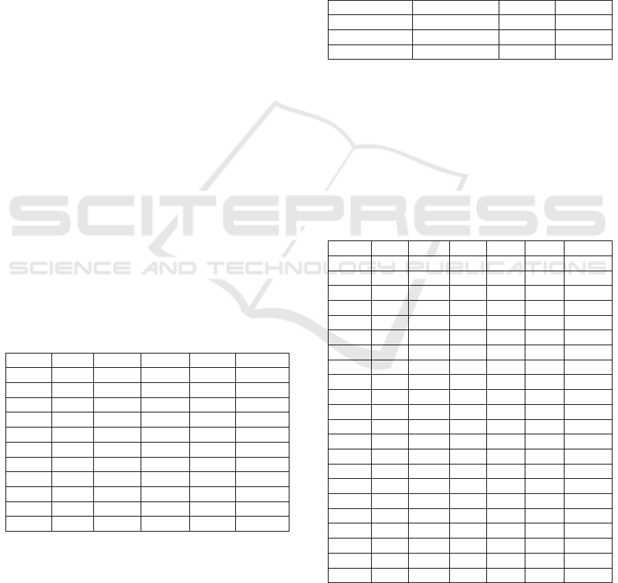
Table 1: CPLEX results of the original model.

ID N Pallets Before After Time(s)

1 7 22 10156 7361 17.47

2 5 23 7934 5593 MLR

3 5 18 7166 6072 3.05

4 2 22 7890 5398 MLR

5 2 32 11090 9805 MLR

6 7 23 8295 6065 MLR

7 7 33 10012 9898 18.25

8 2 14 4638 3100 MLR

9 2 8 3054 2600 0.18

10 3 4 1461 1461 0.16

SUM

71703 57355

103.91

For the current model formulation, we solved 5

out of 10 instances to optimality within 200s time

limit. The average computation time is 103.91s. The

reduction in delivery cost is 20%. The reduction in

cost is promising for the business, but the

computational time is a bit long for daily business, as

we need to save enough time for the operations and

actual loading. The row in the table labelled ‘MLR’

means those instances haven’t been solved to

optimality within the time limit and the after cost for

those cost are the current best feasible solution found.

4.1 Example

There are three different trucks available with

different costs. The truck information is shown in

Table 2.

Table 2: Trucks Information.

ID Length Width Price

10T 9.6 2.4 2600

18T 13.5 2.5 4100

20T 16.5 2.5 4300

We have 22 pallets to be packed and 7 different

customers. Three customers are special customers

that needed to be drop off later on route. The packing

results are shown in Table 3. CID is the customer ID,

PID is the pallet ID, l, w, vol are the length, width and

volume of the pallets, TP is the indicator of whether

the customer is telecommunication customer and the

Sol column is the solution.

Table 3: Example One Input Data.

CID PID l w vol TP Sol

1 0 1.65 1.15 4.07 YES LTL

2 1 1.91 1.11 2.79 NO 10T-1

2 2 1.91 1.11 5.29 NO 10T-1

2 3 1.91 1.11 5.29 NO 10T-1

2 4 1.91 1.11 5.29 NO 10T-1

3 5 1.91 1.11 5.29 NO 10T-2

3 6 1.91 1.11 5.29 NO 10T-2

3 7 1.91 1.11 5.29 NO 10T-2

3 8 1.91 1.11 5.29 NO 10T-2

3 9 1.91 1.11 5.29 NO 10T-2

3 10 1.91 1.11 5.29 NO 10T-2

4 11 1.91 1.11 5.29 YES LTL

5 12 1.91 1.11 1.42 NO 10T-1

5 13 1.91 1.11 5.29 NO 10T-1

5 14 1.91 1.11 5.29 NO 10T-1

5 15 1.91 1.11 5.29 NO 10T-1

6 16 1.91 1.11 5.29 NO 10T-2

6 17 1.91 1.11 5.29 NO 10T-2

6 18 1.91 1.11 5.29 NO 10T-2

6 19 1.91 1.11 5.29 NO 10T-2

7 20 1.41 1.15 3.04 YES LTL

7 21 1.41 1.15 3.04 YES LTL

The visualizations of the packing results are

shown in Figure 3 and Figure 4. We can see that the

optimal solution is a mix of LTL and FTL shipping.

Decision Support for Bundle Shipment Choices: Orthogonal Two-dimensional Bin Packing with Practical Constraints

165

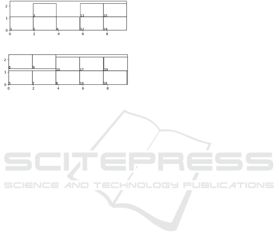
The optimal cost is 7361.64 while the original

shipping with all pallets shipped LTL is 10156.95. A

28% reduction in delivery cost is achieved in this

instance within 7.2 seconds.

Figure 3: Packing Result of Example (10T Truck No.1).

Figure 4: Packing Result of Example (10T Truck No.2).

5 ENHANCE SOLVING

EFFICIENCY

A careful formulation for a mixed integer program

(MIP) can lead to a solution of the mathematical

model in a reasonable amount of time, while some

formulations of the same problem can make the

model practically unsolvable. The key principle of a

better formulation of a MIP model is to make the

feasible region of LP relaxation model as tight as

possible even if this will make the LP model harder

to solve. This topic is covered in various text books

(Nemhauser and Wolsey, 1988; Williams, 1990). In

this paper, we consider improving the solving

efficiency by tailored fixed charges in the MIP,

reducing symmetry and a careful implementation of

the MIP model for large cases.

5.1 Tailored Big M

To model a fixed charge—a cost that is incurred once

when a process is used, but is not proportional to the

level of the process—a "Big M" formulation is

usually used. We could choose a sufficiently large

value for M, but there are some drawbacks when

solve the LP relaxation of the MIP problem. If the

relaxation objective value is too far from the integer

objective value; the branching algorithm will try to

force 



to 0 first, because the LP solution value of





is already close to 0. So we need to choose M

carefully; big enough for the bounding purpose but

not too large. The values of M in constraints (2), (3),

(5), (6), (8) and (9) are max



 , max



 ,

max



, max



, 2 and max









respectively.

5.2 Symmetry in Trucks









,∀12

(13)

If k1 and k2 are the same type (same dimension) of

trucks, we would select k1 first to break the

symmetry/tie in trucks. Because select k1 and k2 will

yield the same objective value and create ties in the

candidate solutions.

5.3 Symmetry in Pallets









2











1,∀



,





(14)

If pallet i and pallet j are identical, we would place

pallet j either below pallet i or to the left of pallet i to

break the symmetry. Also, the routing sequence

conditions constraints (9) also help to reduce

symmetry in pallets.

5.4 Sequence Pairs Restriction

To make sure any two pallets do not overlap, they

must not overlap in x axis (one on the left of another

in the graph), or not overlap in y axis (one below

another in the graph), or not overlap in both axis.

Based on this information, we can add two other

constraints to obtain a tighter LP relaxation of the

MIP and make the feasible region described by the

linear programming relaxation as close as possible to

the feasible region that contains only feasible integer

solutions.





















21,∀



(15)





















21,∀



(16)

Constraints (15) and (16) void the other eight

infeasible sequence pairs, meaning the relative

position of two pallets cannot be left and right (top

and bottom) at the same time.

5.5 Pre-grouped Pallets

In this problem, we only consider a small assortment

of pallets size. Pallets of the same type can be

prepacked into a lager item and significantly reduce

the problem sizes. An example was shown in Table 4.

ICORES 2021 - 10th International Conference on Operations Research and Enterprise Systems

166

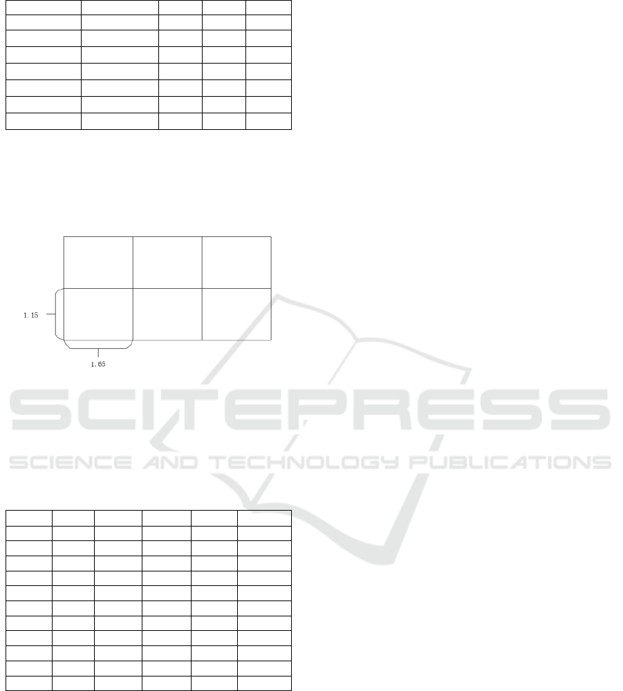
Table 4: A data example after pallets combination.

CID PID l w vol

1 c0 4.95 2.3 24.36

1 c1 4.95 2.3 24.36

2 c2 4.95 2.3 24.36

2 c3 4.95 2.3 24.36

2 c4 4.95 2.3 24.36

2 7 1.65 0.4 0.75

2 11 1.65 0.4 0.75

c0-c4 are prepacked pallets set as shown in Figure

5. The original problem is unsolvable within 200s,

and the modified problem is solved in 0.34s. The

objective value is 7200, which is a 35.13% saving in

delivery cost than before.

Figure 5: 6-blocks Pattern (Pre-combined Pallets).

We rerun the modified model with all techniques

proposed in section 5.1 – section 5.5 for the ten test

cases in Table 1 and the new results are shown in

Table 5.

Table 5: CPLEX results of the modified model.





Pallets Before After Time(s)

1 7 22 10156 7361 3.57

2 5 23 7934 5593 0.84

3 5 18 7166 6072 4.05

4 2 22 7890 5898 0.9

5 2 32 11090 7200 0.34

6 7 23 8295 5707 0.91

7 7 33 10012 9898 1.69

8 2 14 4638 3100 0.58

9 2 8 3054 2600 0.18

10 3 4 1461 1461 0.16

SUM

71703 54892

1.32

With the new formulated mathematical model and

the 6-blocks patterns generation, we can solve all ten

instances to optimality within 200s time limit. The

average computation time is now only 1.322s. The

reduction in delivery cost is 23.45%. We reduce the

computational time significantly and it could be

applied in the real life business. We also did stress test

of this model with CPLEX. The original problems are

solved by commercial solver CPLEX to optimality up

to 34 pallets within 200s. For the modified version of

the model, the solvability is increased to 154 pallets.

6 CONCLUSIONS

In this paper, we study a problem where a

telecommunication equipment company sends

products from warehouses to customer sites in

mainland China once a day by truck. There are two

types of truck delivery service: less-than-truckload

(LTL) shipping and full-truckload (FTL) shipping.

We help the company to make the decisions on the

type of shipping to choose, number of trucks needed

for FTL as well as the loading sequence and positions

of products onto each truck. We modelled the

problem as a variant of an orthogonal 2D-BPP using

mixed-integer linear programing (MIP) with the

objective to minimise the total cost of delivery. It

combines two discrete optimization problems: Bin

packing and optimal bundle shipment decisions.

Hence we model this as an integrated mixed integer

programing model (MIP) with two sets of constraints,

one for bin packing the other for bundle shipment cost

computation. The problem is solved using the

CPLEX solver. Experiment results are carried out to

demonstrate the performance of the new model.

A 26% of reduction in delivery cost is achieved

by applying this model in real life cases. Also, we

provided some practical guidance on how to

reformulate the problem with care to improve the

solving efficiency. We solved the reformulated model

on the same numerical examples and reduced

computational time to 1.3 seconds on average and

help the model to be implemented for a real life

business.

REFERENCES

Buljubašić, M. and Vasquez, M., 2016. Consistent

neighborhood search for one-dimensional bin packing

and two-dimensional vector packing. Computers &

Operations Research, 76, pp.12-21.

Christofides, N. and Whitlock, C., 1977. An algorithm for

two-dimensional cutting problems. Operations

Research, 25(1), pp.30-44.

Cui, Y. P., Yao, Y. and Zhang, D., 2017. Applying triple-

block patterns in solving the two-dimensional bin

packing problem. Journal of the operational research

society, pp.1-14.

Dyckhoff, H. and Wäscher, G., 1990. Cutting and packing

(special issue). European Journal of Operational

Research, 44(2).

Decision Support for Bundle Shipment Choices: Orthogonal Two-dimensional Bin Packing with Practical Constraints

167

Garey, M. R. and Johnson, D.S., 1979. Computers and

intractability (Vol. 174). San Francisco: freeman.

Lins, L., Lins, S. and Morabito, R., 2002. An n-tet graph

approach for non-guillotine packings of n-dimensional

boxes into an n-container. European Journal of

Operational Research, 141(2), pp.421-439.

Lodi, A., Martello, S. and Monaci, M., 2002. Two-

dimensional packing problems: A survey. European

journal of operational research, 141(2), pp.241-252.

Lodi, A., Monaci, M. and Pietrobuoni, E., 2017. Partial

enumeration algorithms for two-dimensional bin

packing problem with guillotine constraints. Discrete

Applied Mathematics, 217, pp.40-47.

Martello, S. and Vigo, D., 1998. Exact solution of the two-

dimensional finite bin packing problem. Management

science, 44(3), pp.388-399.

Martins, G. H., 2003. Packing in two and three dimensions.

Naval Postgraduate School Monterey CA Dept of

Operations Research.

Murata, H., Fujiyoshi, K., Nakatake, S. and Kajitani, Y.,

2003. Rectangle-packing-based module placement. In

The Best of ICCAD (pp. 535-548). Springer, Boston,

MA.

Pisinger, D. and Sigurd, M., 2007. Using decomposition

techniques and constraint programming for solving the

two-dimensional bin-packing problem. INFORMS

Journal on Computing, 19(1), pp.36-51.

Polyakovskiy, S. and M’Hallah, R., 2020. Just-in-time two-

dimensional bin packing. Omega, p.102311.

Scheithauer, G. and Sommerweiß, U., 1998. 4-block

heuristic for the rectangle packing problem. European

Journal of Operational Research, 108(3), pp.509-526.

Williams, H. P., 1990. Integer and combinatorial

optimization. Journal of the Operational Research

Society, 41(2), pp.177-178.

Wolsey, L. A. and Nemhauser, G. L., 1999. Integer and

combinatorial optimization (Vol. 55). John Wiley &

Sons.

ICORES 2021 - 10th International Conference on Operations Research and Enterprise Systems

168