Driver’s Eye Fixation Prediction by Deep Neural Network

Mohsen Shirpour, Steven S. Beauchemin and Michael A. Bauer

Department of Computer Science, The University of Western Ontario, London, ON, N6A-5B7, Canada

Keywords:

Driver’s Eye Fixation, Saliency Region, Convolution Neural Network, Eye Tracking, Trafﬁc Driving.

Abstract:

The driving environment is a complex dynamic scene in which a driver’s eye ﬁxation interacts with trafﬁc scene

objects to protect the driver from dangerous situations. Prediction of a driver’s eye ﬁxation plays a crucial

role in Advanced Driving Assistance Systems (ADAS) and autonomous vehicles. However, currently, no

computational framework has been introduced to combine the bottom-up saliency map with the driver’s head

pose and gaze direction to estimate a driver’s eye ﬁxation. In this work, we ﬁrst propose convolution neural

networks to predict the potential saliency regions in the driving environment, and then use the probability of the

driver gaze direction, given head pose as a top-down factor. We evaluate our model on real data gathered during

drives in an urban and suburban environment with an experimental vehicle. Our analyses show promising

results.

1 INTRODUCTION

Recently, visual driver attention has become a no-

ticeable element of intelligent Advanced Driver As-

sistance Systems (i-ADAS) to increase trafﬁc safety.

Based on the World Health Organization (WHO)

studies, approximately 1.35 million fatalities and any-

where between 20 to 50 million injuries occur every

year on the roads. The WHO predicts that road trafﬁc

accidents will rise to become the ﬁfth primary reason

for mortality in 2030 (Organization et al., 2018). Ev-

idence has shown that a considerable number of acci-

dents are due to distraction.

Driver monitoring research has been carried out

for years in various research ﬁelds, from science to

engineering, to protect the driver from dangerous situ-

ations. The driver’s eye ﬁxation plays a crucial role in

the research on Driver Safety System and Enhanced

Driver Awareness (EDA) systems to alert drivers on

incoming trafﬁc conditions and warn them appropri-

ately. Some driver monitoring systems use head and

eye location to evaluate the driver’s gaze-direction

and gaze-zone (Zabihi et al., 2014; Shirpour et al.,

2020). Their purpose is to estimate the driver’s intent

and predict the driver’s maneuvers a few seconds be-

fore they occur (Khairdoost et al., 2020; Jain et al.,

2015). Their results illustrate a strong connection be-

tween a driver’s visual attention and action.

The driver’s eye generally ﬁxates on parts of the

driving environment that depend on a number of ob-

jective and subjective factors that are based on two

classes of attentional mechanisms: bottom-up and

top-down. Bottom-up mechanisms consider features

obtained from the driving scene such as trafﬁc signs,

vehicles, trafﬁc lights, and so on. In contrast, top-

down mechanisms are driven by internal factors such

as a driver’s experience or intent (Deng et al., 2016).

Saliency maps identify essential regions in the scene

(Cazzato et al., 2020). In a driving context, top-down

factors signiﬁcantly contribute to the estimation of

trafﬁc saliency maps, which in turn provides an in-

sight as to what a driver’s gaze may be ﬁxated on

while driving.

In this study, we focus on developing a framework

to predict the driver’s eye ﬁxation onto the forward

stereo system’s imaging plane located on the instru-

mented vehicle’s rooftop. This paper is structured as

follows: an overview on the current literature in the

ﬁeld of saliency regions is provided in Section 2, fol-

lowed by a description of the RoadLAB vehicle in-

strumentation and data collection processes in Section

3. Section 4 describes our proposed method. In Sec-

tion 5, we present and evaluate the experimental re-

sults. We provide a conclusion and areas for further

research in Section 6.

2 RELATED WORKS

Trafﬁc saliency methods focus on highlighting salient

regions or areas in a given environment. This is an

active area in the ﬁelds of computer vision and intel-

ligent vehicle systems. We provide a summary of the

literature that brings the essential concepts of visual

Shirpour, M., Beauchemin, S. and Bauer, M.

Driver’s Eye Fixation Prediction by Deep Neural Network.

DOI: 10.5220/0010220800670075

In Proceedings of the 16th International Joint Conference on Computer Vision, Imaging and Computer Graphics Theory and Applications (VISIGRAPP 2021) - Volume 4: VISAPP, pages

67-75

ISBN: 978-989-758-488-6

attention and salient regions applied to driving envi-

ronments.

Saliency, as it relates to visual attention, refers

to areas of ﬁxation humans or drivers would con-

centrate on at a ﬁrst glance. The modern history of

visual saliency goes back to the works of Itti (Itti

et al., 1998). They considered low-level features,

namely intensity, color, and orientation at multiple

scales extracted from images, and then normalized

and combined with linear and non-linear methods to

estimate a saliency map. (Harel et al., 2007) sug-

gested a saliency method based on Graph-Based Vi-

sual Saliency (GBVS). They deﬁned the equilibrium

distribution of Markov chains from low-level features

and then combined them to obtain the ﬁnal saliency

map. (Schauerte and Stiefelhagen, 2012) proposed

quaternion-based spectral saliency methods that ap-

ply the integration of quaternion DCT and FFT-based

to estimate spectral saliency for predicting human eye

ﬁxations. (Li et al., 2012) proposed a bottom-up fac-

tor for visual saliency detection, which is considered

a scale-space analysis of amplitude spectra of images.

They convolved image spectra with properly scaled

low-pass Gaussian kernels to obtain saliency maps.

(Deng et al., 2016) demonstrated that a driver’s at-

tention was mainly focused on the vanishing points

present in the scene. They applied the road vanish-

ing point as guidance for the trafﬁc saliency detection.

Subsequently, they proposed a model based on a ran-

dom forest to predict a driver’s eye ﬁxation according

to low-level features (color, orientation, intensity) and

vanishing points (Deng et al., 2017). Details on low-

level features for non-deep learning approaches are

provided in (Borji et al., 2015).

Deep learning-based models brought a paradigm

shift in computer vision research. Deep-learning

methods commonly perform better when compared

with classical learning methods. (Vig et al., 2014)

introduced one of the early networks that performed

large scale searches over different model conﬁgura-

tions to predict saliency regions. (Liu et al., 2015)

proposed Multi-resolution Convolutional Neural Net-

works (Mr-CNN) to learn two types of visual features

from images simultaneously. The Mr-CNNs were

trained to classify image regions for saliency at differ-

ent scales. Their model used top-down feature factors

learned in upper-level layers, and bottom-up features

gathered by a combination of information over vari-

ous resolutions. They then integrated bottom-up and

top-down features with a logistic regression layer that

predicted eye ﬁxations. (K

ummerer et al., 2016) pre-

sented the DeepGaze model that applied the VGG-19

deep neural network for feature extraction, where fea-

tures for saliency prediction were extracted without

any additional ﬁne-tuning. (Huang et al., 2015) pro-

posed a deep neural network (DNN) obtained from

concatenating two pathways: the ﬁrst path considered

a large scale image to extract coarse features, and the

second path considered a smaller image scale to ex-

tract ﬁne ones. This model and similar ones are suit-

able to extract features at various scales. (Wang and

Shen, 2017) proposed a framework that extracted fea-

tures from deep coarse-layers with global information

and shallow ﬁne layers with local information that

captured hierarchical saliency features to predict eye

ﬁxation. Subsequently, they designed the Attentive

Saliency Network (ASNet) from the ﬁxations to de-

tect salient objects (Wang et al., 2019).

In the driving context, (Palazzi et al., 2018) pro-

posed a model based on a multi-branch deep neural

network on the DR(eye)VE dataset, which consisted

of three-stream convolutional networks for color, mo-

tion, and semantics. Each stream possessed its param-

eter set, and the ﬁnal map aggregated a three-stream

prediction. Also, (Tawari and Kang, 2017) estimated

drivers’ visual attention with the use of a Bayesian

Network model and detected the saliency region with

a fully convolutional neural network. (Deng et al.,

2019) proposed a model to detect driver’s eye ﬁxa-

tions based on a convolutional-deconvolutional neu-

ral network (CDNN). Their framework could predict

the primary ﬁxation location and was able to predict

the second saliency region in the driving context, if it

existed.

This contribution aims to apply a Deep Neural

Network to our natural driving sequence for the esti-

mation of saliency maps followed by a Gaussian Pro-

cess Regression (GPR) to estimate the driver’s con-

ﬁdence region for the ﬁnal estimation of driver’s eye

ﬁxation.

3 VEHICLE INSTRUMENTATION

AND DATA COLLECTION

3.1 Vehicle Conﬁguration

Our experimental vehicle is equipped with a stereo

system placed on the vehicle’s roof to capture the

frontal driving environment. A remote eye-gaze

tracker located on the dashboard captures several fea-

tures related to the driver, including head position and

orientation, left and right gaze Euler angles, and left

and right eye center locations within the coordinate

system of the tracker. Furthermore, the On-Board Di-

agnostic system (OBD-II) records the current status of

vehicular dynamics such as vehicle speed, brake and

VISAPP 2021 - 16th International Conference on Computer Vision Theory and Applications

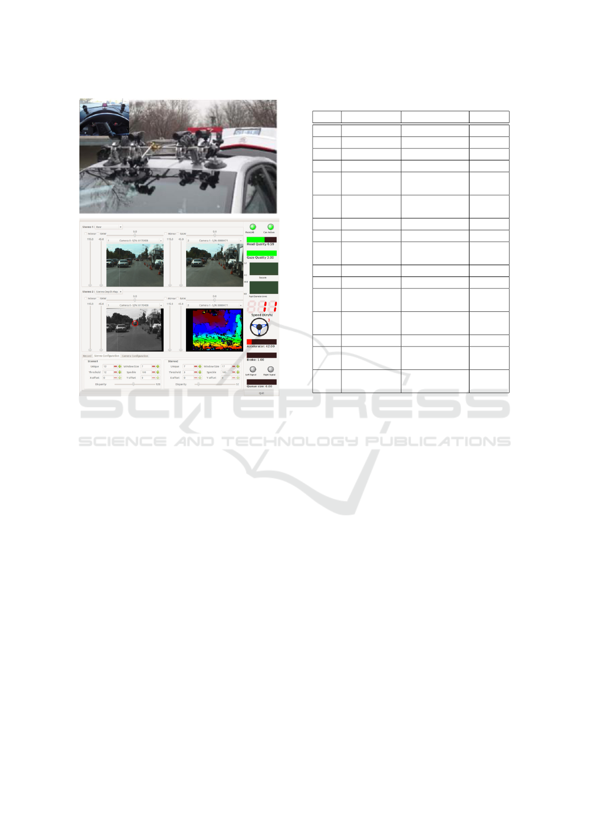
Figure 1: RoadLAB conﬁguration. (top): vehicular con-

ﬁguration: stereoscopic vision system on rooftop and 3D

infrared eye-tracker located on the dashboard. (bottom):

software systems: The on-board system displays frame se-

quences with depth maps, dynamic vehicle features, and

eye-tracker data.

accelerator pedal pressure, steering wheel angle, etc.

Figure 1 depicts the RoadLAB experimental vehicle

and its software systems as described in (Beauchemin

et al., 2011).

3.2 Cross-calibration Technique

The calibration process between the eye-tracker and

stereo system is essential for generating a useful Point

of Gaze (PoG). We applied a technique developed in

our laboratory to cross-calibrate these systems and

project the PoGs onto the stereo system imaging

plane. Details are provided in (Kowsari et al., 2014).

3.3 Participants

Sixteen drivers participated in this experiment, in-

cluding nine females and seven males. The partici-

pants drove frequently. Each participant was recorded

by our instrumented vehicle on a pre-determined

28.5km route within the city of London, ON, Canada.

Table 1: Description of Data.

Seq# Date Weather Gender

1 2012-08-24 29

◦

C Sunny M

2 2012-08-24 31

◦

C Sunny M

3 2012-08-30 23

◦

C Sunny F

4 2012-08-31 24

◦

C Sunny M

5 2012-09-05 27

◦

C Par-

tially Cloudy

6 2012-09-10 21

◦

C Par-

tially Cloudy

7 2012-09-12 21

◦

C Sunny F

8 2012-09-12 27

◦

C Sunny M

9 2012-09-17 24

◦

C Par-

tially Cloudy

10 2012-09-19 8

◦

C Sunny M

11 2012-09-19 12

◦

C Sunny F

12 2012-09-21 18

◦

C Par-

tially Cloudy

13 2012-09-21 19

◦

C Par-

tially Cloudy

14 2012-09-24 7

◦

C Sunny F

15 2012-09-24 13

◦

C Par-

tially Cloudy

16 2012-09-28 14

◦

C Par-

tially Cloudy

Each sequence represented a driving time of ap-

proximately one hour. Sequences were recorded

in different circumstances, including scenery (down-

town, urban, suburban) and trafﬁc conditions vary-

ing from low-trafﬁc to high-trafﬁc situations. They

were recorded in various weather conditions (sunny,

partially-cloudy, cloudy) and at various times of the

day (see Table 1).

3.4 Driver Gaze-movement Analysis

Our eye-tracker performed the gaze estimation and

provided a conﬁdence measure on its quality. This

metric ranged from 0 to 3, and we considered the

driver’s gaze to be reliable when this metric had a

value of 2 or higher. We selected the PoGs projected

onto the vehicle’s forward stereo system in the pre-

ceding 15 consecutive frames. The driver’s PoG data

implemented with the Gaussian distribution (Figure 2

) were considered the ground-truth data.

4 DRIVER FIXATION

We proposed method to predict a driver’s eye ﬁxation

in the forward stereo vision reference frame. First,

we introduce a model to predict the saliency maps in

Driver’s Eye Fixation Prediction by Deep Neural Network

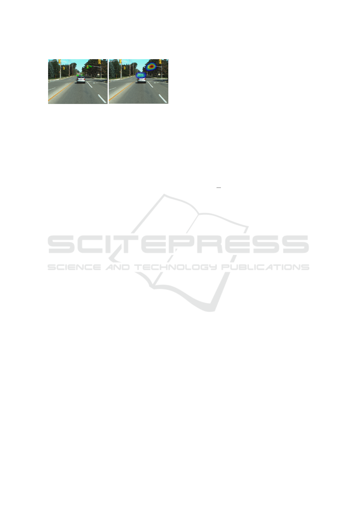
Figure 2: An example of PoG and matching ﬁxation

saliency map. (left): PoGs projected onto the forward

stereo system of the vehicle obtained with the preceding 15

consecutive frames. (right): The driver’s point of gaze as a

2-D Gaussian distribution.

the driving scene, inspired by (Wang and Shen, 2017).

Following this, we use a framework proposed in our

laboratory to estimate the probability of driver’s gaze

direction, as top-down information for prediction of

driver’s eye ﬁxation (Shirpour et al., 2020).

4.1 Model Architecture

The network conﬁguration selection is a fundamen-

tal step when using a neural network. There are

various types of deep neural network saliency mod-

els, mainly divided into three groups: single stream,

multi-stream, and skip layer networks. Our network

inherits the advantage of skip layer networks capa-

ble of capturing hierarchical features. This network

conﬁguration learns multi-scale features inside the

model; the low-level layers reﬂect primitive features

such as edges, corners, etc; and the high-level layers

represent meaningful information such as parts of ob-

jects in various positions. The network architecture is

shown in Figure 3. This architecture promotes perfor-

mance via:

• The creation of multi-scale saliency features in-

side the network.

• The preservation of high-resolution features from

the encoder path

Our network encoder is based on the ﬁrst ﬁve

convolutional layers of VGG16 (Simonyan and Zis-

serman, 2014), used for feature extraction from in-

put images. The dimensions of the input images are

H × W × 3. The network encoder includes a stack

of convolution layers that gradually learns from local

to global information. The spatial feature dimensions

generated from VGG16 are consequently divided by

2 until, in the last convolution layers, the dimensions

reach H/16 × W /16. We choose three feature maps

from the encoder path generated by convolution lay-

ers ConV 3 − 3, ConV 4 − 3, and ConV 5 − 3 to capture

multi-scale saliency information. We use these three-

channel feature maps with different dimensions and

resolutions to obtain the ﬁnal saliency prediction.

In the decoder part for each path, we apply multi-

ple deconvolution layers to increase the spatial dimen-

sion toward getting a saliency prediction map with di-

mensions identical to those of the input images. For

instance, the feature map in the ConV 3− 3 layer has a

H/4× W /4 spatial dimension (after each convolution

block, the spatial dimension size is halved). Its de-

coder network path includes two deconvolution lay-

ers, where the ﬁrst one doubles the spatial size of fea-

ture map to H/2 × W /2, while the second deconvo-

lution increases the spatial size of the feature map to

H × W . Each deconvolution in these paths is followed

by a Rectiﬁed Linear Unit ReLU layer, which learns

a nonlinear upsampling. Similarly, the other decoder

path related to ConV 4 − 3 and ConV 5 − 3 layers has

three and four deconvolution layers, respectively.

The loss function L(S

) is deﬁned as follows:

L(S

) =

∑

n=1

log(S

)+(1 − S

)log(1− S

)

(1)

where N is the number of pixels, S

is the i

pixel

from the ground truth driver’s ﬁxation map, and S

the i

pixel from the predicted driver’s ﬁxation map.

4.2 Top-down Information

The driver gaze is not explicitly related to the head

pose due to the interaction between head and eye

movements. Generally, the driver moves both the

head and the eyes to obtain a ﬁxation. In our previ-

ous research, we suggested a stochastic model for de-

scribing a driver’s visual attention. This method uses

a Gaussian Process Regression (GPR) approach that

estimates the driver gaze direction probability, given

head pose. We refer the reader to (Shirpour et al.,

2020) for details on the conﬁdence interval for the

driver’s gaze direction process.

Based on the driver’s head pose information, we

propose a trafﬁc saliency maps framework, which uti-

lizes the gaze direction as a top-down constraint. The

primary part of the framework is to ﬁnd top-down

features according to the driver’s head pose and to

estimate the probability of a driver’s gaze direction,

which is then fused with the saliency map, as follows:

(x,y) = wS

(x,y) + (1 − w)S

(x,y) (2)

where w is the weighting factor, S

(x,y) represents

the conﬁdence interval of driver’s gaze according to

the head pose information, and S

(x,y) represents the

saliency map model. The weight w in (2) is a critical

parameter of the framework, as it dictates the impor-

tance of the top-down factor in our model. To choose

a correct weight, we have shown that the drivers focus

VISAPP 2021 - 16th International Conference on Computer Vision Theory and Applications

+ +

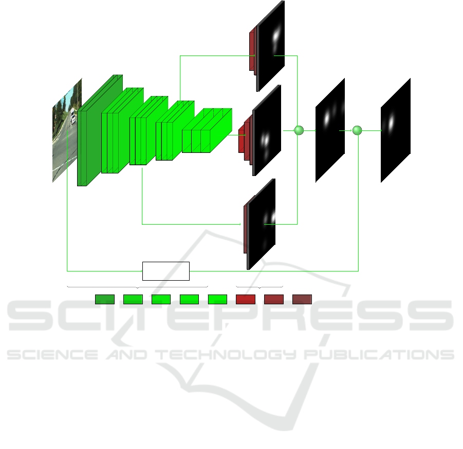
GPR: Driver gaze direction

Encoder Decoder

ConV1 ConV2 ConV3 ConV4 ConV5 DeConV1 DeConV2 DeConV3

Figure 3: Network conﬁguration.

most of their attention on the 95% conﬁdence interval

region estimated with the driver head pose. Since, the

top-down saliency area includes 80% of the informa-

tion that is related to a driver’s ﬁxation within the area

of the conﬁdence interval of the driver’s head pose,

we hypothesized that 0.8 was a suitable value for w.

5 EXPERIMENTAL EVALUATION

In this section, we describe the training of our pro-

posed network and evaluate its performance both

qualitatively and quantitatively.

5.1 Qualitative Evaluation

To evaluate our model against a number of cutting-

edge methods, we chose various sample frames from

challenging driving environments, including difﬁcult

situations and conditions, such as trafﬁc objects with

different sizes, low contrast scenes, and multiple traf-

ﬁc objects. Figure 4 illustrates the comparison of our

network against other methods, namely: Graph-based

Visual Saliency (GBVS) (Harel et al., 2007), Image

Signature (Hou et al., 2011), Itti (Itti et al., 1998), and

Hypercomplex Fourier Transform (HFT) (Li et al.,

2012). Results clearly demonstrate that our method

highlights the drivers’ ﬁxation areas more accurately

and preserves details compared to other methods. Our

model displays excellent prediction of trafﬁc objects

such as trafﬁc signs, trafﬁc lights, pedestrians, vehi-

cles, among others. Other models displayed difﬁcul-

ties when attempting to detect relevant information

from the driving environments. Conversely, by way

of bottom-up and top-down processes, our model ac-

curately predicts the driver’s ﬁxation, including the

primary and secondary ﬁxation, if they exist.

5.2 Quantitative Evaluation Metrics

We have evaluated our model’s performance on vari-

ous metrics to measure the correspondence between

the driver’s eye ﬁxation prediction and the ground

truth driver’s eye ﬁxation.

Some of the metrics considered herein are based

on the location of ﬁxation, such as Normalized Scan-

path Saliency (NSS) (Peters et al., 2005), and Area

under ROC Curve (AUC-Borji (Borji et al., 2012),

AUC-Judd (Judd et al., 2012)). They evaluate the sim-

ilarity between the driver’s eye ﬁxation prediction and

Driver’s Eye Fixation Prediction by Deep Neural Network

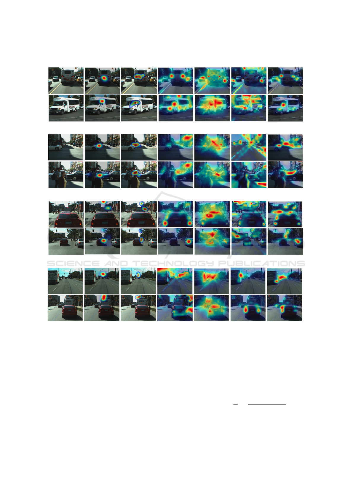
Large Trafﬁc Objects.

Low-Contrast and Shadows.

Multiple Trafﬁc Objects.

Small Trafﬁc Objects.

Input frame Fixation map Proposed Itti GBVS Image signature HFT.

Figure 4: We selected results from the RoadLab dataset from different driving scenes, including large, small, and multiple

trafﬁc objects, in addition to low contrast scenes, to better show the processing capability of each approach. (from left to

right:) input frames, ground truth ﬁxation maps, our predicted saliency maps, and the predictions of Itti (Itti et al., 1998),

GBVS (Harel et al., 2007), Image Signature (Hou et al., 2011), and HFT (Li et al., 2012).

ground-truth. In contrast, others are based on distri-

butions, such as Earth Movers Distance (EMD) (Pele

and Werman, 2008), Similarity Metric (SIM) (Judd

et al., 2012), and Linear Correlation Coefﬁcient (CC)

(Le Meur et al., 2007). They evaluate the dissimilar-

ity between the model’s prediction and ground truth.

Let S

represent the ground-truth driver’s eye ﬁxation

map and S

the saliency maps prediction provied by

the various methods:

• Normalized Scanpath Saliency (NSS): The NSS

metric is computed by the average normalized

saliency at driver’s eye ﬁxation locations, as fol-

lows:

NSS =

∑

n=1

) − µ

(3)

where N is the number of eye positions, (x

)

the eye-ﬁxation point location, and µ

, and σ

VISAPP 2021 - 16th International Conference on Computer Vision Theory and Applications

Table 2: Saliency metric scores of our model as compared with state-of-the-art saliency models on the RoadLab dataset.

Models NSS CC SIM AUC-

Borji

AUC-

Judd

EMD

GT 3.26 1 1 0.88 0.94 0

ITTI (Itti et al., 1998) 1.15 0.23 0.25 0.62 0.64 2.13

GBVS (Harel et al., 2007) 1.32 0.29 0.32 0.69 0.71 1.91

Image Signature (Hou et al., 2011) 1.48 0.29 0.30 0.73 0.75 2.06

HFT (Li et al., 2012) 1.42 0.42 0.38 0.64 0.66 2.31

∆QDCT (Schauerte and Stiefelha-

gen, 2012)

1.68 0.34 0.32 0.71 0.73 1.72

RARE2012 (Riche et al., 2013) 1.34 0.31 0.33 0.67 0.68 1.48

ML Net (Cornia et al., 2016) 2.47 0.72 0.66 0.76 0.80 1.43

Wang (Wang and Shen, 2017) 2.87 0.78 0.68 0.81 0.85 1.23

Proposed 2.98 0.82 0.72 0.81 0.89 1.06

are the mean and standard deviation of a driver’s

eye ﬁxation map predication.

• Area Under the ROC Curve (AUC): AUC is

commonly used for evaluating estimated saliency

maps. With AUC, two types of locations are con-

sidered: the true driver ﬁxation points, regarded

as the positive set, versus a negative set consisting

of the sum of other ﬁxation points. The driver’s

eye ﬁxation map is classiﬁed into the salient and

non-salient regions with a predetermined thresh-

old. Then, the ROC curve is plotted by the true-

positive (TP) rate versus the false-positive (FP)

rate, as the threshold varies from 0 to 1. De-

pending on the non-ﬁxation distribution’s selec-

tion, there are two commonly used types of AUC,

namely AUC-Judd and AUC-Borji.

• Linear Correlation Coefﬁcient (CC): The CC

provides a measure of the linear relationship be-

tween S

and S

. This metric varies between −1

and 1, and a value close to either −1 or 1 shows

alignment between S

and S

CC =

cov(S

)

× σ

(4)

• Similarity Metric (SIM): This metric estimates

the similarity between the distributions of pre-

dicted and ground truth driver’s eye ﬁxation maps

by measuring the intersection between two distri-

butions, calculated by a sum of the minimum val-

ues at any pixel location from distributions (S

(n)

and S

(n)):

SIM =

∑

n=1

min(S

(n),S

(n)) (5)

where, S

(n) and, S

(n) are normalized distribu-

tions, and N is the number of locations of inter-

est in the maps. A value close to 1 indicates that

the two saliency maps are similar, while the score

close to zero denotes little overlap.

• Earth Mover’s Distance (EMD): This metric

computes the spatial distance between two proba-

bility distributions S

(n) and S

(n) over a region,

as the minimum cost of transforming the probabil-

ity distribution of the computed driver’s eye ﬁxa-

tion map S

(n) into the ground truth S

(n). A

high value for EMD indicates little similarity be-

tween the distributions.

To illustrate the effectiveness of the saliency map

model in predicting a driver’s eye ﬁxation, we com-

pared our model with eight state-of-the-art tech-

niques, including six non-AI models: ITTI (Itti et al.,

1998), GBVS (Harel et al., 2007), Image Signature

(Hou et al., 2011), HFT (Li et al., 2012), RARE2012

(Riche et al., 2013), ∆QDCT (Schauerte and Stiefel-

hagen, 2012), and two deep learning-based models:

ML-Net (Cornia et al., 2016), and Wang (Wang and

Shen, 2017). These models have been introduced in

Driver’s Eye Fixation Prediction by Deep Neural Network

recent years and are often utilized for comparison pur-

poses.

The quantitative results obtained on the RoadLAB

dataset (Beauchemin et al., 2011) are presented in Ta-

ble 2. Our proposed model gives the maximum sim-

ilarity and minimum dissimilarity with respect to the

ground truth data. We conclude that our model pre-

dicts the driver’s eye ﬁxation maps more accurately

than other saliency models.

6 CONCLUSIONS

We proposed convolution neural networks to predict

the potential saliency maps in the driving environ-

ment, and then employed our previous research re-

sults to estimate the probability of the driver gaze di-

rection, given head pose as a top-down factor. Fi-

nally, we statistically combined bottom-up and top-

down factors to obtain accurate drivers’ ﬁxation pre-

dictions.

Our previous study established that driver gaze es-

timation is a crucial factor for driver maneuver predic-

tion. The identiﬁcation of objects that drivers tend to

ﬁxate on is of equal importance in maneuver predic-

tion models. We believe that the ability to estimate

these aspects of visual behaviour constitutes a signiﬁ-

cant improvement for the prediction of maneuvers, as

drivers generally focus on environmental features a

few seconds before affecting one or more maneuvers.

REFERENCES

Beauchemin, S. S., Bauer, M. A., Kowsari, T., and Cho, J.

(2011). Portable and scalable vision-based vehicular

instrumentation for the analysis of driver intentional-

ity. IEEE Transactions on Instrumentation and Mea-

surement, 61(2):391–401.

Borji, A., Cheng, M.-M., Jiang, H., and Li, J. (2015).

Salient object detection: A benchmark. IEEE trans-

actions on image processing, 24(12):5706–5722.

Borji, A., Sihite, D. N., and Itti, L. (2012). Quantitative

analysis of human-model agreement in visual saliency

modeling: A comparative study. IEEE Transactions

on Image Processing, 22(1):55–69.

Cazzato, D., Leo, M., Distante, C., and Voos, H. (2020).

When i look into your eyes: A survey on computer

vision contributions for human gaze estimation and

tracking. Sensors, 20(13):3739.

Cornia, M., Baraldi, L., Serra, G., and Cucchiara, R. (2016).

A deep multi-level network for saliency prediction.

In 2016 23rd International Conference on Pattern

Recognition (ICPR), pages 3488–3493. IEEE.

Deng, T., Yan, H., and Li, Y.-J. (2017). Learning to boost

bottom-up ﬁxation prediction in driving environments

via random forest. IEEE Transactions on Intelligent

Transportation Systems, 19(9):3059–3067.

Deng, T., Yan, H., Qin, L., Ngo, T., and Manjunath, B.

(2019). How do drivers allocate their potential at-

tention? driving ﬁxation prediction via convolutional

neural networks. IEEE Transactions on Intelligent

Transportation Systems, 21(5):2146–2154.

Deng, T., Yang, K., Li, Y., and Yan, H. (2016). Where does

the driver look? top-down-based saliency detection in

a trafﬁc driving environment. IEEE Transactions on

Intelligent Transportation Systems, 17(7):2051–2062.

Harel, J., Koch, C., and Perona, P. (2007). Graph-based vi-

sual saliency. In Advances in neural information pro-

cessing systems, pages 545–552.

Hou, X., Harel, J., and Koch, C. (2011). Image signa-

ture: Highlighting sparse salient regions. IEEE trans-

actions on pattern analysis and machine intelligence,

34(1):194–201.

Huang, X., Shen, C., Boix, X., and Zhao, Q. (2015). Sali-

con: Reducing the semantic gap in saliency prediction

by adapting deep neural networks. In Proceedings of

the IEEE International Conference on Computer Vi-

sion, pages 262–270.

Itti, L., Koch, C., and Niebur, E. (1998). A model of

saliency-based visual attention for rapid scene anal-

ysis. IEEE Transactions on pattern analysis and ma-

chine intelligence, 20(11):1254–1259.

Jain, A., Koppula, H. S., Raghavan, B., Soh, S., and Saxena,

A. (2015). Car that knows before you do: Anticipating

maneuvers via learning temporal driving models. In

Proceedings of the IEEE International Conference on

Computer Vision, pages 3182–3190.

Judd, T., Durand, F., and Torralba, A. (2012). A benchmark

of computational models of saliency to predict human

ﬁxations.

Khairdoost, N., Shirpour, M., Bauer, M. A., and Beau-

chemin, S. S. (2020). Real-time maneuver prediction

using lstm. IEEE Transactions on Intelligent Vehicles.

Kowsari, T., Beauchemin, S. S., Bauer, M. A., Lauren-

deau, D., and Teasdale, N. (2014). Multi-depth cross-

calibration of remote eye gaze trackers and stereo-

scopic scene systems. In 2014 IEEE Intelligent

Vehicles Symposium Proceedings, pages 1245–1250.

IEEE.

ummerer, M., Wallis, T. S., and Bethge, M. (2016).

Deepgaze ii: Reading ﬁxations from deep fea-

tures trained on object recognition. arXiv preprint

arXiv:1610.01563.

Le Meur, O., Le Callet, P., and Barba, D. (2007). Predict-

ing visual ﬁxations on video based on low-level visual

features. Vision research, 47(19):2483–2498.

Li, J., Levine, M. D., An, X., Xu, X., and He, H. (2012). Vi-

sual saliency based on scale-space analysis in the fre-

quency domain. IEEE transactions on pattern analy-

sis and machine intelligence, 35(4):996–1010.

Liu, N., Han, J., Zhang, D., Wen, S., and Liu, T. (2015). Pre-

dicting eye ﬁxations using convolutional neural net-

works. In Proceedings of the IEEE Conference on

Computer Vision and Pattern Recognition, pages 362–

370.

VISAPP 2021 - 16th International Conference on Computer Vision Theory and Applications

Organization, W. H. et al. (2018). Global status report on

road safety 2018: Summary. Technical report, World

Health Organization.

Palazzi, A., Abati, D., Solera, F., Cucchiara, R., et al.

(2018). Predicting the driver’s focus of attention: the

dr (eye) ve project. IEEE transactions on pattern anal-

ysis and machine intelligence, 41(7):1720–1733.

Pele, O. and Werman, M. (2008). A linear time histogram

metric for improved sift matching. In European con-

ference on computer vision, pages 495–508. Springer.

Peters, R. J., Iyer, A., Itti, L., and Koch, C. (2005). Compo-

nents of bottom-up gaze allocation in natural images.

Vision research, 45(18):2397–2416.

Riche, N., Mancas, M., Duvinage, M., Mibulumukini, M.,

Gosselin, B., and Dutoit, T. (2013). Rare2012: A

multi-scale rarity-based saliency detection with its

comparative statistical analysis. Signal Processing:

Image Communication, 28(6):642–658.

Schauerte, B. and Stiefelhagen, R. (2012). Quaternion-

based spectral saliency detection for eye ﬁxation pre-

diction. In European Conference on Computer Vision,

pages 116–129. Springer.

Shirpour, M., Beauchemin, S. S., and Bauer, M. A. (2020).

A probabilistic model for visual driver gaze approx-

imation from head pose estimation. In 2020 IEEE

3nd Connected and Automated Vehicles Symposium

(CAVS). IEEE.

Simonyan, K. and Zisserman, A. (2014). Very deep con-

volutional networks for large-scale image recognition.

arXiv preprint arXiv:1409.1556.

Tawari, A. and Kang, B. (2017). A computational frame-

work for driver’s visual attention using a fully convo-

lutional architecture. In 2017 IEEE Intelligent Vehi-

cles Symposium (IV), pages 887–894. IEEE.

Vig, E., Dorr, M., and Cox, D. (2014). Large-scale opti-

mization of hierarchical features for saliency predic-

tion in natural images. In Proceedings of the IEEE

Conference on Computer Vision and Pattern Recogni-

tion, pages 2798–2805.

Wang, W. and Shen, J. (2017). Deep visual attention pre-

diction. IEEE Transactions on Image Processing,

27(5):2368–2378.

Wang, W., Shen, J., Dong, X., Borji, A., and Yang, R.

(2019). Inferring salient objects from human ﬁxations.

IEEE transactions on pattern analysis and machine

intelligence.

Zabihi, S., Beauchemin, S. S., De Medeiros, E., and Bauer,

M. A. (2014). Frame-rate vehicle detection within the

attentional visual area of drivers. In 2014 IEEE Intel-

ligent Vehicles Symposium Proceedings, pages 146–

150. IEEE.

Driver’s Eye Fixation Prediction by Deep Neural Network