Non-linear Monte Carlo Ray Tracing for Visualizing Warped Spacetime

Avirup Mandal

∗

, Kumar Ayush

∗

and Parag Chaudhuri

Indian Institute of Technology Bombay, Powai, Mumbai, India

Keywords:

Raytracing, Non-linear Monte Carlo, Warped Spacetime, Relativity.

Abstract:

General relativity describes the curvature of spacetime. Rays of light follow geodesic paths in curved space-

time. Visualizing scenes containing spacetime regions with pronounced curvature requires tracing of these

light ray paths. We present a Monte Carlo approach for non-linear raytracing to render scenes in curved space-

time. In contrast to earlier work, we can accurately resolve ray-object interactions. This allows us to create

plausible visualizations of what happens when a black hole appears in a more known environment, like a room

with regular specular and diffuse surfaces. We demonstrate that our solution is correct at cosmological scales

by showing how spacetime warps around a stationary Schwarzschild black hole and a non-stationary Kerr

black hole. We verify that the solution is consistent with the predictions of general relativity. In the absence

of any curvature in spacetime, our renderer behaves like a normal linear ray tracer. Our method has the poten-

tial to create rich, physically plausible visualizations of complex phenomena that can be used for a range of

purposes, from creating visual effects to making pedagogical aids to understand the behaviour of spacetime as

predicted by general relativity.

1 INTRODUCTION

General relativity changed the way in which we un-

derstand our universe. The theory presented by Ein-

stein in 1915 has been veriﬁed via multiple experi-

mental observations. However, the concept of curved

spacetime that is central to this theory stays elusive to

a casual reader. Even students of physics have trouble

visualizing what curved spacetime looks like because

it is so far removed from our daily experience. It was

only recently that a visualization of curved spacetime

was created that is true as per general relativity and it

depicted how a black hole would look to an observer

much closer to it (James et al., 2015a) (James et al.,

2015b). The cosmological phenomenon visualized in

these works were a rotating black hole and a worm-

hole.

A black hole can be described as a region in space

where the gravitational ﬁeld is so strong that no matter

or radiation can escape. The boundary of the region

from which no escape is possible is called the event

horizon. According to the general theory of relativity,

a body of sufﬁcient mass can deform or warp space-

time around it and result in a black hole. A static black

hole, which possesses no electric charge or angular

∗

A. Mandal and K. Ayush contributed equally to this

work.

momentum is referred to as a Schwarzschild black

hole (Schwarzschild, 1916). A Kerr black hole (Kerr,

1963) on the other hand, possesses angular momen-

tum and rotates. Another related cosmological phe-

nomenon is a wormhole, which is like a hole punched

through curved spacetime connecting two different

regions of spacetime. An example of this is the Ellis

Wormhole, visualized in the movie Interstellar (Ellis,

1973) (Morris and Thorne, 1988) (Thorne, 2015).

The curving of spacetime, however, is a fact pre-

dicted by the theory of general relativity and is present

in the vicinity of any object that has mass. We are in-

terested in visualizing not only black holes, but any

warped spacetime, both at cosmological and at earth-

like or everyday scales. We present in this paper a ray

tracing method that allows us to visualize any arbi-

trary scene in any type of spacetime. We can stochas-

tically trace rays in the warped spacetime, while tak-

ing care of normal light-surface interactions like re-

ﬂection and refraction. This allows us to visualize ev-

eryday geometry in strongly curved spacetimes. We

believe our work is ﬁrst of its kind in being able to

create such visualizations. We ﬁnd the images that

our renderer produces to be extremely useful in un-

derstanding the concept of curved spacetime and vi-

sualizing how the universe behaves in the presence of

gravity. We also believe it is unique in being able to

Mandal, A., Ayush, K. and Chaudhuri, P.

Non-linear Monte Carlo Ray Tracing for Visualizing Warped Spacetime.

DOI: 10.5220/0010217600760087

In Proceedings of the 16th International Joint Conference on Computer Vision, Imaging and Computer Graphics Theory and Applications (VISIGRAPP 2021) - Volume 3: IVAPP, pages 76-87

ISBN: 978-989-758-488-6

create physics-based visualizations that are of interest

to generating special effects in cinema and as such,

it is intended to work as a proof of concept that ray

tracing in curved spacetime can easily be integrated

into existing production pipelines. As a result, now

we may have more realistic wormholes opening up in

an alley in New York, which acts as a pathway for

aliens. The major contributions of our work are listed

as below

• We perform secondary ray tracing and resolve all

object-ray intersections in curved space-time.

• We render our scene using complete global illumi-

nations in warped spacetime which is essential to

produce visual phenomena like soft shadows and

caustics.

• We develop a non-linear ray tracing algorithm that

works both in cosmological as well as terrestrial

scale.

We talk about relevant current literature in the next

section. We explain light paths in curved spacetime,

and derive expressions for the geodesics that repre-

sent the light paths in Section 3. We present partic-

ular solutions for the Schwarzschild and Kerr met-

rics for non-rotating and rotating black holes respec-

tively, and for the Ellis metric for wormholes. Then

we present our simple ray integrator in Section 4. De-

tailed results and discussions of the results are pre-

sented in Section 5.

2 RELATED WORK

Astrophysical ray tracers have a long history. These

visualizations have become adept at simulating and

visualizing increasingly complex cosmological phe-

nomena. Gas, dust and other stellar debris that has

come close to a black hole but not quite fallen into

it, forms a ﬂattened band of spinning matter around

the event horizon called the accretion disk. Thin ac-

cretion disks around black holes were visualized in

early work in the area (Luminet, 1979). Subsequent

works added color (Fukue and Yokoyama, 1988),

handled rotating black holes and thicker accretion

disks (Viergutz, 1993) and ﬁnally images produced

by a simulated camera ﬂyby near the disk (Marck,

1996). The special relativistic visualization of 4D

space (Müller et al., 2010) and visualization of circu-

lar motion around Schwarzschild black hole (Müller

and Boblest, 2011) have been explored before. The

general relativistic ray tracer GYOTO (Vincent et al.,

2011) uses the Hamiltonian formalism to integrate

the rays backward in time. They also compute the

speciﬁc intensity that reaches the observer by in-

tegrating the radiative transfer equation along the

computed geodesic. However, they assume the ob-

jects to be emissive, as most astrophysical objects

of interest in such extreme environments are, and do

not handle reﬂection and refraction from those ob-

jects, specular or diffuse. Another work presented by

Müller (Müller, 2014) uses the Motion4D library to

handle spacetime metrics and ray tracing. The GPU

accelerated renderer presented in GRay (Chan et al.,

2013) (Kuchelmeister et al., 2012) further parallelizes

the work presented in earlier literature, to increase the

throughput at which rays can be traced. Another GPU

based renderer (Weiskopf et al., 2004) discusses re-

fraction through a continuous medium of varying re-

fractive index as an example on non-linear ray tracing,

but does not tackle refraction within a warped space-

time itself.

Among other work, is also the Black Hole Flight

Simulator (BHFS) (Hamilton, 2008), that shows how

it looks like to travel towards and through various

kinds of black holes. A ray tracing algorithm for

visualizing two different spinning celestial objects, a

neutron star and a quasi-Kerr black hole are described

in (Psaltis and Johannsen, 2012) and (Bauböck et al.,

2012) respectively.

It was only recently that visualizations with an

observer placed closer to the black hole were pro-

duced. The Double Negative Gravitational Renderer

(DNGR) was used to produce the imagery for the

acclaimed movie Interstellar (Thorne, 2015) (James

et al., 2015a) (James et al., 2015b). The renderer

is unique in that it not only solves the equations for

a ray-bundle propagation near a spinning black hole,

but also produces extremely high resolution imagery

required for a cinema production. This is done by

mapping the celestial sphere around a black hole or

a wormhole to the local sky of the observing camera,

while accounting for the change in the cross-section

of the light beam and, color and intensity changes due

to Doppler shifts that occur in the process.

2.1 Comparison to State of the Art

We do not claim to present any new astrophysics

insights in our paper, nor do we claim to be bet-

ter than DNGR in all respects. We certainly do not

produce cinematic production quality images. How-

ever, we believe that to the best of our knowledge,

we present the only renderer of its kind that can vi-

sualize highly warped spacetime, both in outer space

and in everyday human-scale scenes like rooms and

buildings. None of the previous works (Müller,

2014), (Kuchelmeister et al., 2012), (James et al.,

Non-linear Monte Carlo Ray Tracing for Visualizing Warped Spacetime

2015a), (James et al., 2015b) deal with simulating

complete global illumination in curved spacetime.

In contrast, we can perform secondary ray trac-

ing and accurately resolve ray-object intersection in

curved spacetime. This allows us to perform global

illumination and render complex scenes that consist

of specular and diffuse surfaces. Thus unlike previous

works, we can generate soft shadows, caustics etc in

curved spacetime. Moreover, we use bidirectional ray

tracing for the regions where less number of primary

rays reach and perform local smoothing for regions

with high numerical error. Prior work like (Müller

et al., 2010) and (Müller and Boblest, 2011) deal with

non-linear raytracing in a restrictive class of space-

time. Our method can handle any spacetime topology.

Visualizing the warping of spacetime around fa-

miliar geometries that represent our everyday experi-

ences provides an unique perspective from which to

understand curved spacetime, which leads us to claim

that our renderer has unique pedagogical value for

the casual science enthusiast who wants to understand

general relativity, and to teachers and students of the

subject. It is also of immense use to CGI profession-

als who have to architect such spacetimes for special

effects in their productions, while staying true to its

physics underpinnings.

3 LIGHT PATHS IN CURVED

SPACETIME

Black

Hole

Primary ray from star

Secondary ray from star

Ray surface from caustic, through Einstein Ring to camera

Einstein Ring

Camera sky

Celestial

Sphere

Caustic

Star

Figure 1: Schematic diagram showing the bending of light

rays around a black hole.

Here we present the underlying theory behind deriv-

ing the light paths in curved spacetime, as dictated by

general relativity. In layman terms, all objects with

mass bend spacetime with the curvature being pro-

portional to their mass. Objects like neutron stars and

black holes, which have a lot of mass or energy, gener-

ate strong enough gravitational forces to warp space-

time in a very pronounced manner.

The warping of light rays around a black hole is

schematically shown in Figure 1. Two light rays ema-

nating from a star on the celestial sphere are deﬂected

around opposite sides of the black hole due to warp-

ing of spacetime. This will happen to all the stars on

the celestial sphere near the black hole and this phe-

nomena is known as gravitational lensing. The Ein-

stein ring is an image of a point source that is on the

celestial sphere, diametrically opposite to the camera.

This point is the Caustic point, and the orange surface

shows the locus of rays from this point converging at

the camera. The Einstein ring is the intersection of

these rays with the camera sky. For the star we will

see two images in the camera sky, one inside the Ein-

stein ring and the other outside it.

The principle of least action dictates that light rays

follow geodesics in this curved spacetime. In order to

generate the image of the curved spacetime due to the

distortions produced in it by gravitational inﬂuence

of phenomena like black holes, we must trace these

geodesic paths. We derive the expressions for these

geodesic paths, from principles of general relativity.

The notation used here is the index notation and

Einstein summation convention used in general rela-

tivity. These have been explained in Appendix A. In-

terested readers can refer (Misner et al., 1973) (Hartle,

2003) (Collier, 2013)for more details.

Distance between two points in a spacetime is

given by a metric. If the Minkowski metric is η

αβ

then proper time, τ can be written as

dτ

= η

αβ

dξ

(1)

where proper time is the time measured by an ob-

server in their own rest frame. The Principle of Equiv-

alence of Gravitation and Inertia states that at every

spacetime point in an arbitrary gravitational ﬁeld it is

possible to choose a locally inertial coordinate sys-

tem such that, within a sufﬁciently small region of the

point in question, the laws of nature take the same

form as in an accelerated Cartesian coordinate system

in the absence of gravitation. Therefore, for a parti-

cle moving purely under the inﬂuence of gravitational

forces, there is a freely falling coordinate system ξ

in which its equation of motion is that of a straight

line in spacetime (or equivalently is a geodesic of the

spacetime). This can be written as

dτ

= 0 (2)

Considering any other coordinate system x

, the

freely falling coordinates ξ

can be considered to be

functions of x

, and Equation 2 can be re-written as

dτ



∂ξ

∂x

dτ



= 0 (3)

∂ξ

∂x

dτ

∂

∂x

dτ

= 0 (4)

IVAPP 2021 - 12th International Conference on Information Visualization Theory and Applications

Multiplying this by

∂x

∂ξ

and simplifying, gives us

the equation of motion of the particle as

dτ

+ Γ

µν

dτ

= 0 (5)

where Γ

µν

is the connection coefﬁcient or Christoffel

symbol, deﬁned by

µν

∂x

∂ξ

∂

∂x

(6)

Since light rays travel along null geodesics, i.e.,

paths on which proper time does not change, dτ =

0, we replace dτ with another parameter ζ to get the

geodesic equation that gives us the path of the light

ray. In such a case, ζ represents the afﬁne parameter

that varies along the geodesic.

dζ

+ Γ

µν

dζ

= 0 (7)

3.1 The Hamiltonian Formulation

The (Euler-Lagrange) geodesic equation derived in

the previous section, though analytically perfect is not

amenable to numerical simulation. For that purpose,

we use a Hamiltonian formulation of the equation of

motion. If we note that proper time can be written in

an arbitrary coordinate system in terms of the metric

tensor as

dτ

= g

µν

dξ

(8)

where g

µν

is deﬁned as

µν

∂ξ

∂x

∂ξ

∂x

αβ

(9)

Now, a Hamiltonian can be constructed from the

metric of the (pseudo-Reimannian) manifold repre-

senting the spacetime as

H (x

, p

) =

µν

) p

(10)

Here g

µν

are the contravariant terms of the metric, x

is the coordinate of the photon travelling along the ray

and p

is the generalized momentum.

The equations of motion can now be written as

dζ

∂H

∂p

= g

αν

(11)

d p

dζ

= −

∂H

∂x

= −

∂g

µν

∂x

(12)

It can be proved that these equations are to-

gether equivalent to Equation 7. This form makes

it easy for us to write 6 ﬁrst order differential equa-

tions for the 6 variables of motion (three coordi-

nates, three momenta), which can then be integrated

to get the ray path. We can solve these equations

for any given spacetime metric. In the next section,

we present the solutions for the Schwarzschild, Kerr

and Ellis metrics, which describe spacetime around a

Schwarzschild black hole, Kerr black hole and Ellis

worm hole respectively. In the all the metric equa-

tions discussed below, we have assumed light speed

c = 1.

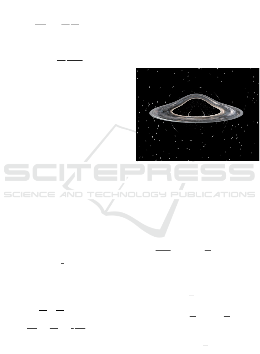
Figure 2: Here we can see an accretion disk rendered around

a Schwarzschild black hole rendered using our ray tracer.

3.1.1 The Schwarzschild Metric Solution

The Schwarzschild solution was the ﬁrst exact solu-

tion to the Einstein ﬁeld equations (Schwarzschild,

1916). It describes a static, spherically symmetric,

gravitational ﬁeld in the empty region of spacetime

near a massive spherical object. In isotropic coordi-

nates, the metric is given by



1 −

1 +



−



1 +





+ dy

+ dz



(13)

Here r

is the Schwarzschild radius, r

= 2GM , where

G is the gravitational constant and M is the mass of

the body. R is the radius of the spherical body. The

contravariant metric tensor can thus be written as

µν

= diag



1 −

1 +



,−



1 +



−



1 +



,−



1 +





(14)

Now, for α = 0, x

≡t, the equations of motion, Equa-

tions 11 and 12 give

dζ



1 +

1 −



(15)

Non-linear Monte Carlo Ray Tracing for Visualizing Warped Spacetime

d p

dζ

= 0 (16)

The second of these equations implies that p

is a con-

stant, and thus we can conveniently choose p

= −1

to get

dζ

= −



1 −

1 +



(17)

We similarly write for α = 1, 2,3 the equations

dζ

= −



1 +



−4

(18)

d p

dζ



+ p





1 +





1 +





1 −



(19)

Using the equation for

dζ

, we can obtain



1 +



−6



1 −



(20)

d p

= −





+ p





1 −





1 +





1 −







−1



(21)

Since there is no cross dependence amongst coor-

dinate evaluations, we can normalize p

, and it does

not make any difference to integration, except chang-

ing the functions by a scale factor. It just results in

time re-scaling, and does not affect us for a static vi-

sualization.

We integrate Equations 20 and 21, to get the path

of the light ray in a spacetime near a Schwarzschild

black hole. An example of a scene with a

Schwarzschild black hole can be seen in Figure 7.

Figure 2 shows a realistic looking accretion disk

where the warping of spacetime bends the disk and

makes it appear around the Schwarzschild black hole.

The solution for other metrics can be similarly de-

rived, and therefore we can handle any arbitrary met-

ric representing a spacetime.

3.1.2 The Kerr Metric Solution

The Kerr metric describes the geometry of empty

spacetime around a rotating, uncharged, axially-

symmetric black hole. In spherical coordinates the

Kerr metric (Chandrasekhar, 2002) for a mass M ro-

tating with angular momentum J is given as

= ρ

∆

−



dφ −

2aMr



sin

−

∆

−ρ

dθ

(22)

where a = J/M, ρ

= r

cos

θ, ∆ = r

−2Mr +

, δ = sin

θ, Σ



+ a



−a

∆δ.

Here, the contravariant metric tensor is given by

µν







1 −

2Mr

0 0

2aMrsin

0 −

∆

0 0

0 0 −ρ

2aMrsin

0 0

−



+ a

Mr sin



sin







(23)

Evaluating the Hamiltonian, as explained in Sec-

tion 3.1, we get the rate of change of position with

time as

∆



dζ



(24)

dθ



dζ



(25)

dφ

2aMrsin

+ p



1 −

2Mr



+ a

) +

2aMrsin

sin

θ − p

2aMrsin

(26)

where

dζ

is deﬁned as

dζ



1 −

2Mr

h

+ a

) +

2aMr sin

sin

θ +



2aMr sin



+ a

) +

2aMr sin

sin

θ − p

2aMr sin

(27)

The rate of change of momentum with time is simi-

larly obtained as

d p

= M



−r

+ a

sin



−2aM sin



−r

+ a

sin



∆r −ρ

(r −M)

∆

˙r

+ r



r + a

M sin



−r

+ a

sin



sin

(28)

d p

Mr sinθ cosθ

−

4aMr(ρ

sinθcosθ + a

sin

θcosθ)

−

sinθcosθ

∆

˙r

−a

sinθcosθ



+ a

)sinθcosθ





(2ρ

sin

θcosθ + a

sin

θcosθ)



(29)

IVAPP 2021 - 12th International Conference on Information Visualization Theory and Applications

d p

= 0 (30)

d p

= 0 (31)

where ˙x =

dτ

for any variable x.These equations are

stable for numerical integration, except at the poles

θ = 0 and θ = π. In this formulation, p

and p

are

conserved along the ray. The ray has two more con-

served quantities as explained below. These are the

axial angular momentum, B

and total angular mo-

mentum, B

. We use these two quantities to track the

stability of the numerical integration during path trac-

ing.

= −

+ cos



sin

−a



(32)

One can verify that the solution of Kerr black hole

metric reduces to the solution of Schwarzschild black

hole metric when a = 0. Thus, as the value of a, i.e.,

angular momentum per unit mass increases, the ro-

tational energy present in the black holes increases.

Now as per Einstein’s general theory of relativity, this

rotational energy term contributes to the mass of the

black hole. Thus the effective mass of a Kerr black

hole is more than it’s original/irreducible mass. It can

be proved (Chandrasekhar, 2002) that the total mass

equivalent M of the black hole including its rotational

energy and its irreducible mass M

irr

are related by

M = 2

irr

−

(33)

As a result when

varies from 0.0 to 1.0 the equiv-

alent mass of Kerr black hole varies from M = M

irr

to M =

√

irr

. So the spacetime distortion is greater

for the Kerr black hole which has a higher

ratio

which in turn implies more rotational energy. We

demonstrate the variation of this distortion in Fig-

ure 10.

3.1.3 The Ellis Metric Solution

The Einstein ﬁeld equations have valid solutions that

contain wormholes. A wormhole is like a tunnel be-

tween two points in spacetime. One of the earliest

known traversable wormholes is the Ellis wormhole.

The Ellis wormhole metric (Ellis, 1973), in spherical

coordinates, is given by

= dt

−dl

−r



dθ

+ sin

θdφ



(34)

where r is a function of the coordinate l, deﬁned as

r =

+ l

and ρ is a constant.

The Hamiltonian in this case is as follows

H =

− p

−

sin

(35)

Since H is independent of the time parameter t and φ,

and p

are conserved along the ray. The total angu-

lar momentum is also conserved, as the wormhole is

spherical and is given by B = p

sin

. Evaluating

the Hamiltonian, we obtain the equations for the rate

of change of position and momentum along time. Let

dζ

= p

= −1 (36)

which shows that ζ = t, up to a constant, and replac-

ing ζ by t gives us ﬁve equations for l,θ, φ, p

, p

functions of time t, along the ray.

= p

dθ

(37)

dφ

sin

d p

= B

dr/dl

d p

cosθ

sin

(38)

These equations are also stable for numerical integra-

tion, except at the poles θ = 0 and θ = π. Integrating

these gives us the geodesics that the light rays follow

in the spacetime around an Ellis wormhole.

4 IMPLEMENTING RAY-OBJECT

INTERACTIONS IN CURVED

SPACETIME

We use a Monte Carlo path tracer to render curved

spacetime for visualization. An important step in path

tracing is calculating the intersection of the sample

ray with the geometry in the scene. For rays that

travel in a straight line, and hence can be represented

by a one parameter equation, it is easy to ﬁnd closed

form expressions for intersection with simple objects

such as spheres, cylinders, cones and cuboids. Even

complicated geometry can be represented with trian-

gle meshes and a ray-triangle intersection is not hard

to compute.

For warped spacetime, we have to integrate the ray

in time, and even for the simplest of objects, it is of-

ten not possible to ﬁnd an analytic solution for the

intersection. A numerical solution also seems difﬁ-

cult when we want our scheme to be compatible with

a potentially arbitrary set of metrics and geometrical

Non-linear Monte Carlo Ray Tracing for Visualizing Warped Spacetime

objects. We ﬁnd an intersection by integrating the

rays one step along the null geodesic at a time, and

we keep decreasing this step size as we approach an

object until we converge to an intersection within ma-

chine precision.

Therefore, in the overall Monte Carlo path tracing

loop we replace the instantaneous ray directions by

those given by the solution to the null geodesic, as

derived in the previous section, and we step along this

direction as explained in Algorithm 1

Algorithm 1: Path tracing & ray-object intersection in

curved space.

1: while number of iterations < MAXITER do

2: Let the current position along the Ray be x

3: Let current time be t and current time

step be dt.

4: Move forward from this position by integrating

the geodesic, to a new position along the ray y

5: Let ˆn be unit object surface normal.

6: if x

· ˆn 6= y

· ˆn then

7: Find perpendicular distance, δ, to

the object surface from current point.

8: if δ < ε then

9: return radiance and normal at

point on surface.

10: else

11: Reset current position on ray to x

12: dt = dt/2.

13: end if

14: end if

15: end while

16: return no intersection (radiance returned is zero).

In our implementation, ε is deﬁned to 1e−10. We

use a Runge-Kutta Order 4 integrator for our path

tracer. Depending on scene complexity, the maxi-

mum number of iterations (MAXITER) for our exper-

iments varies from 100 to 4000 and our starting time

step size, dt, varies from 10.0 to 0.5. Speciﬁcally,

for generating renders with the Ellis wormhole metric

and Kerr black hole metric, we monitor the constants

for a geodesic, p

, p

and B,B

. These constants

are monitored through the integration and if they de-

viate from the expected values by more than a spec-

iﬁed threshold, we halve the time step for the inte-

gration. If they deviate further than a stricter thresh-

old, we simply terminate the integration for that ray

path (geodesic), and mark the corresponding pixel as

erroneous. We later process these erroneous pixels

through a local smoothing step to improve the image

in the error region. The results of this error correction

can be seen in Section 5.

We also sample our rays on a jittered grid to get

an anti-aliased image. On the CPU, we use OpenMP

to speed up the outermost ray tracing loop by using

omp parallel. Apart from that, the only other point

of note was that to render a image of size 1024 ×768

we had a global work size of 1024 ×768, so one work

item per pixel is used which computes the intensity at

that pixel. Thus, the memory available on the graph-

ics card is a restriction in such a case.

5 RESULTS AND DISCUSSION

Here we present extensive demos of our spacetime

renderer.

5.1 Validation Results

A renderer that claims to render curved spacetime

must also work correctly when spacetime is not

curved, i.e., the trivial solution of the Einstein ﬁeld

equations. So we used a Minkowski metric in our

path integration algorithm, and rendered the Cornell

room. The output exactly matches the expected out-

put of a normal Monte Carlo path tracer that works in

ﬂat spacetime. This is shown in Figure 3.

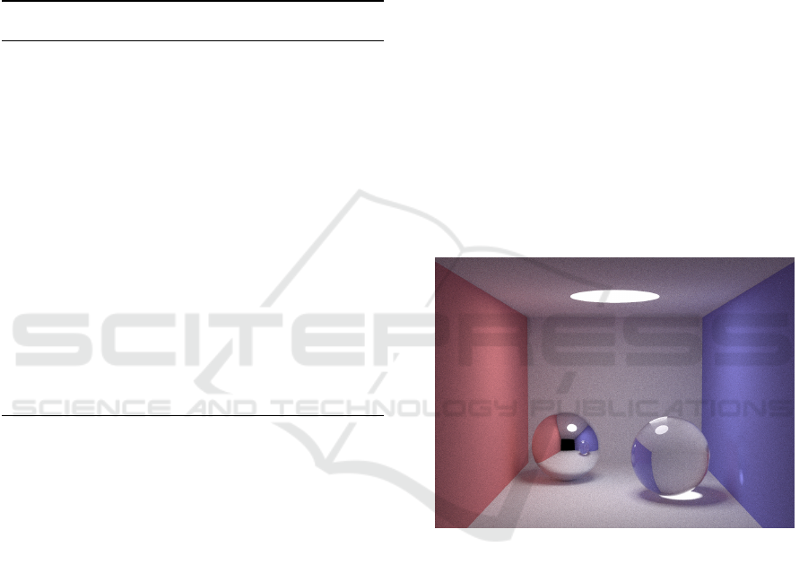
Figure 3: The image of a Cornell box generated by our code

in a ﬂat spacetime, where all rays travel in a straight line.

In order to validate the path tracing in curved

spacetime, we render known models of cosmological

phenomena. We show our simulation of an Einstein

ring, as visualized using our renderer in Figure 4. We

further show our render of gravitational lensing, and

distinct multiple images of a star being produced due

to the phenomena in Figure 5. We can see that the

images of the stars produced by gravitational lensing

are stretched. This is because of the way spacetime

warps around the black hole and the fact that light

paths that start out together spread (or squash) during

the process. If for visual aesthetic reasons we want

stars to only appear as point sources, even in the dis-

torted starﬁeld, it can be achieved by tracing light ray

bundles, instead of single light rays, and then com-

IVAPP 2021 - 12th International Conference on Information Visualization Theory and Applications

puting the effect of spacetime distortion on the cross

sections of these light ray bundles.

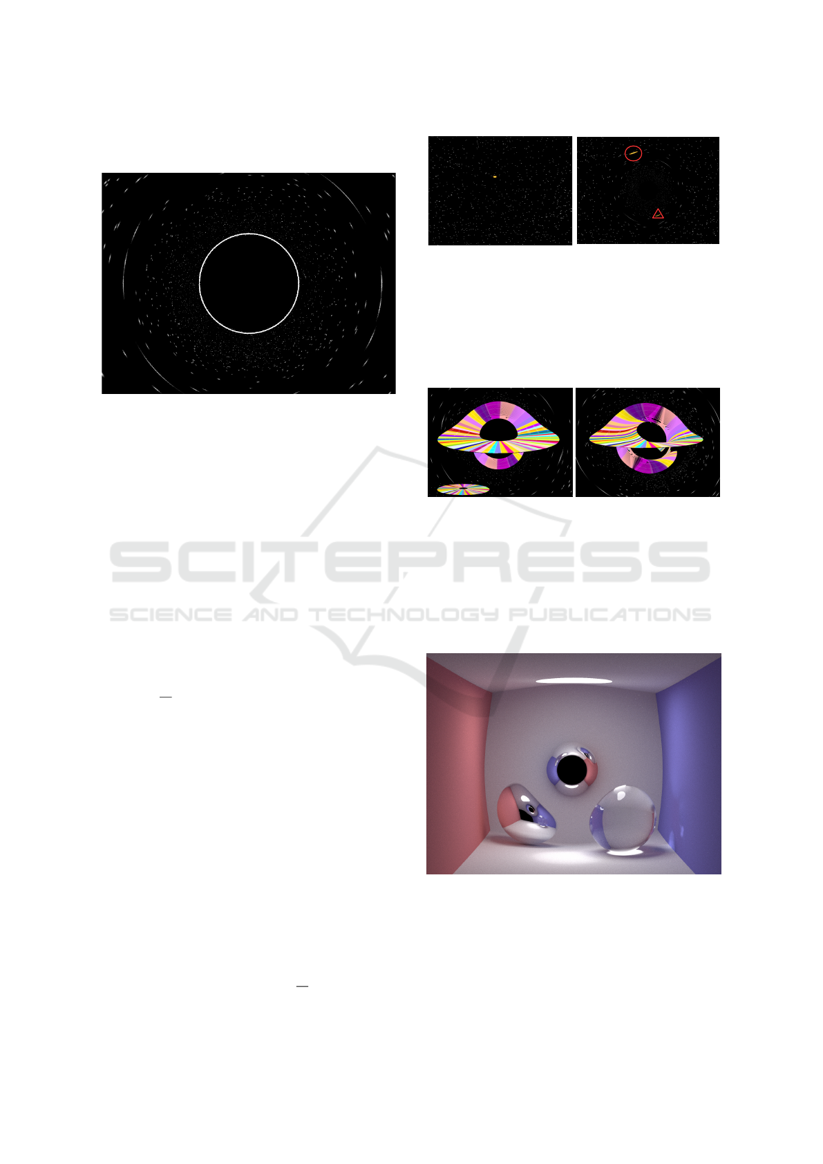
Figure 4: This Einstein ring is produced by placing a light

source behind a black hole diametrically opposite the cam-

era, at the caustic point. We cannot directly see the light

source, but the rays can curve around the black hole to reach

us. The warping of the surrounding starﬁeld follows the pre-

dicted pattern.

We also show the accretion disk around a station-

ary and rotating black hole. Figure 6 shows a thin

accretion disk with a color swatch texture on it being

warped by two different black holes. We can look at

the color of the paint swatch at a location on the disk

and see that parts of the disk are visible more than

once around the black hole. The warping of spacetime

bends the disk and makes it appear around the black

holes. Moreover, the colour patches on the accretion

disk of Kerr black hole appear to be more warped

compared to the Schwarzschild black hole. This is be-

cause of the rotational drag present in the Kerr black

hole. The

ratio of the Kerr black hole is 0.9.

Thus we see that our renderer correctly produces

visualizations of expected cosmological phenomena

as is predicted by the theory of general relativity. We

next demonstrate our results on everyday scenes, ren-

dered in curved spacetime.

5.2 Everyday Scenes around a

Schwarzschild and a Kerr Black

Hole

The everyday scene we choose here is the Cornell

room scene shown in Figure 3. We can see a number

of global illumination phenomena in this room, in-

cluding multiple reﬂections and refractions, caustics,

area lights and soft shadows, and diffuse to diffuse

light transfer. We render a Schwarzschild and multi-

ple Kerr black holes with different

ratio.

Figure 5: Here we can see a starﬁeld warped by a

Schwarzschild black hole. Distinct multiple images of the

same stars can be seen. To illustrate this we have marked a

star in bright yellow in the undistorted starﬁeld image seen

on the left. We can see two images of the bright star in the

starﬁeld warped by the black hole, in the right image. The

primary image of the star is seen on the top, marked by the

red circle and the secondary image of the star is seen on the

bottom, marked by the red triangle.

Figure 6: Here we see an accretion disk around a

Schwarzschild black hole on the left and Kerr black hole

on the right. The undistorted paint swatch texture used on

the disk can be seen on the lower left corner. The black hole

warps spacetime and portions of the same paint swatch ap-

pears both below and above the black hole. This is because

the light rays from the disk are bent by the black hole along

multiple paths and form repeated images. Moreover, in the

rotating black hole straight radial lines on the texture appear

curved due to the more pronounced curvature of spacetime.

Figure 7: The image illustrates a stationary Schwarzschild

black hole of radius 5 units placed right in the center of the

Cornell room.

In Figure 7 we show a Schwarzschild black hole

open in the middle of the room. Notice the bending

of the geometry of the room in the warped space-

time around the black hole. The black hole has a

Non-linear Monte Carlo Ray Tracing for Visualizing Warped Spacetime

event horizon of radius 5 units. The black hole is

in the middle of the room, even in depth, not on the

back wall. In Figure 8, a Schwarzschild black hole

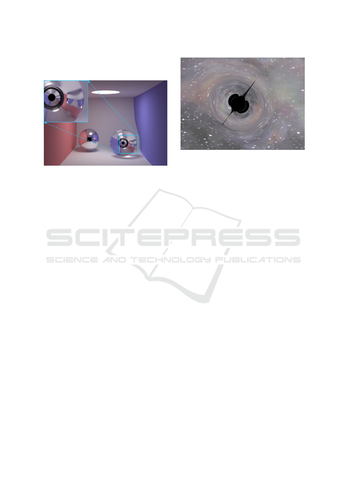
Figure 8: We place a Schwarzschild black hole inside the

refractive glass sphere. We can clearly see the images of the

walls being sucked in towards the center. In the zoomed up

inset image, we can see two images of the room on the right

hand side, both being curved and refracted from different

regions.

of Schwarzschild radius 1.6 units sits inside a refrac-

tive ball of refractive index 1.5 which has a radius of

16 units. The image is formed because of a combi-

nation of the lensing effect by the black hole and the

refraction from the ball’s surface. We can see rings of

darkness in the regions where the black hole directs

light rays at an angle such that they don’t refract out

of the ball, while the lit rings are regions where the

light refracts towards us after being curved from the

black holes. Very notable is the dual image of the re-

fractive ball against the blue background on the right

hand side of the ball. Those rays reﬂect off the re-

ﬂecting ball on the left and then enter again into the

refractive ball, where the black hole curves different

rays from the same part of the scene into different re-

gions of the image, thus allowing us to see multiple

images of the same source. Similar effect can be seen

for a Kerr black hole.

Figure 9 illustrates a warped starﬁeld in presence

of a rotating Kerr black hole with a/M ratio of 0.9.

In Figure 10 we show Kerr black holes with different

a/M ratios, in the middle of the room. The bending

of the geometry of the room in the warped spacetime

around the black hole is more pronounced as the ra-

tio a/M increases. All the black holes have an event

horizon of radius 5 units. Same as before all the black

holes are in the middle of the room (even in depth)

and not on the back wall.

Gravitational lensing, as explained in Section 3 is

seen with streak lines formed by images of stars in the

presence of a moving observer (James et al., 2015a).

We show lensing due to two kinds on black holes in

Figure 9: The image shows a rotating Kerr black hole in a

starﬁeld. Warped spacetime can be clearly seen here along

with phenomena like gravitational lensing.

Figure 11, where we have colored a few lines on the

grid so that we can track where the exact primary and

secondary images are formed.

5.3 Everyday Scenes around an Ellis

Wormhole

We now present our renders for visualizations around

an Ellis wormhole. A wormhole connects two dif-

ferent regions in spacetime, so light rays can travel

through the wormhole from one region to another. In

our ﬁnal sequence of renders, we show a view from a

wormhole, with one end inside the room and the other

end in outer space in Figure 12. A satellite (shown as

the green cylinder) orbits the earth in outer space.

In Figure 13, two images each of both the earth

and the satellite can be seen as crescent shaped disks

in outer space when looked at from the side of the

wormhole that is inside the room. Similarly the room

can be seen when looked at from the side of the worm-

hole that is in space as shown in Figure 12. This

demonstrates that rays of light do correctly bend from

one spacetime region to another, via the wormhole as

is expected.

The view of the room appears dim when seen

through the wormhole end in outer space as in the

Monte Carlo path tracer very few ray samples make

it through the wormhole back to the light source in

the room. This can be corrected by bidirectional path

tracing in curved spacetime, caching the illumination

from the light source to the walls in the room in light

maps stored on the room walls.

The wormhole geodesic solution is not well be-

haved near the poles, as is explained earlier. We ter-

minate the rays near the poles to avoid numerical in-

stability, which causes the black protruding error en-

IVAPP 2021 - 12th International Conference on Information Visualization Theory and Applications

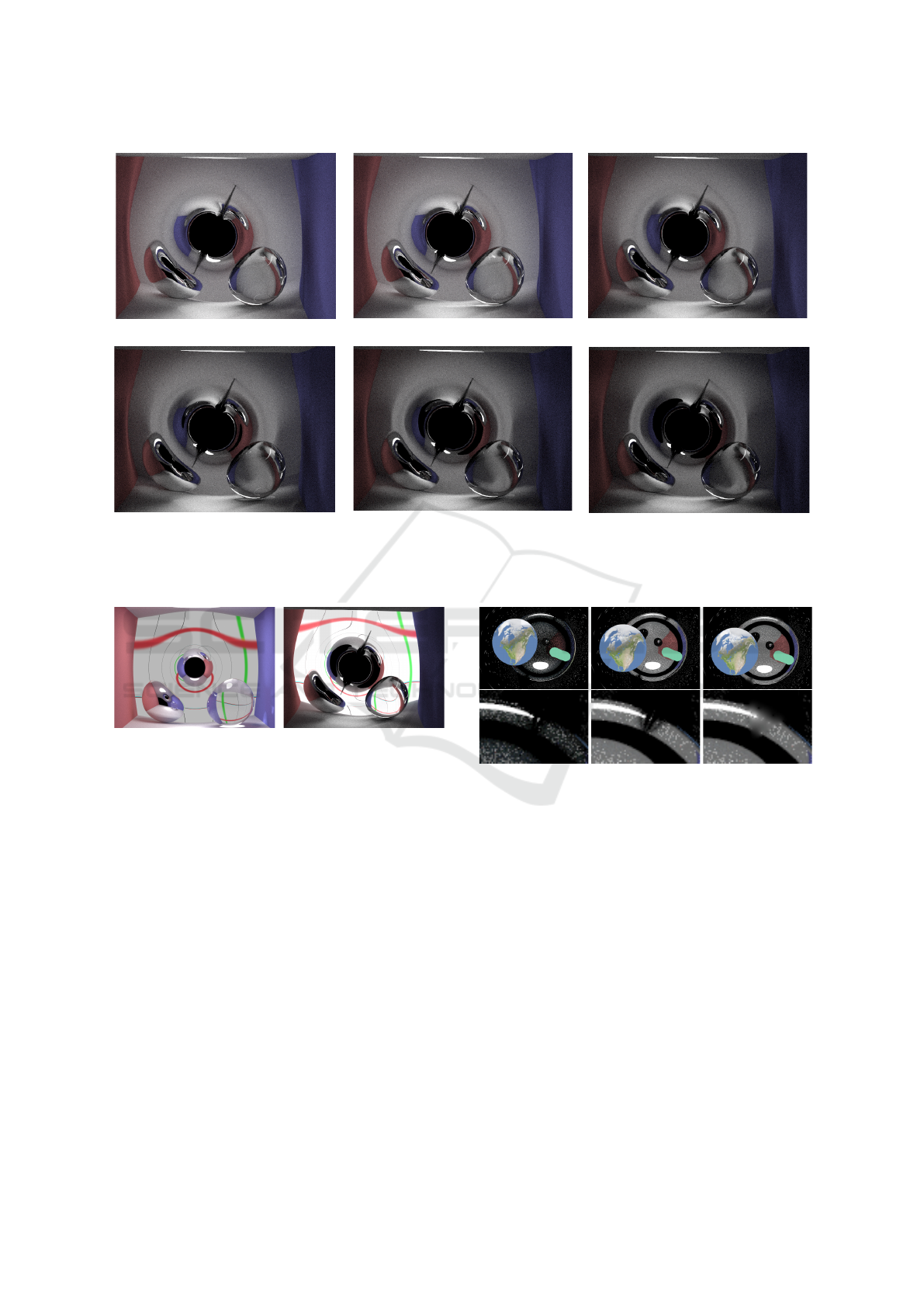
(a) a = 0.5, M = 2.5

(f) a = 2.25, M = 2.5

(b) a = 1.0, M = 2.5

(d) a = 1.75, M = 2.5

(e) a = 2.0, M = 2.5

Figure 10: These are Kerr black holes of radius 5 units and varying a/M ratios placed right in the center of the Cornell room.

In the left, the spacetime distortion is less as the black hole has a lower a/M ratio compared to right one. In the right image

the distortion is so high that the light is not able to reach everywhere in the scene, thus giving the image a darker appearance.

(a) Schwarzschild Black Hole

(b) Kerr Black Hole

Figure 11: Here we show another example of gravitational

lensing rendered by our path tracer for two kinds of black

holes. A rectangular grid has been mapped on the back wall

of the room, on which we have coloured one horizontal line

red and one vertical line green. The red band on top of the

black hole is the primary image of the red line, whereas the

curved red line at the bottom that starts and end at the black

hole, is the secondary image of the red line. Similarly, the

green line to the right is the primary image, and to the left

is the secondary image. Moreover for Kerr black hole the

spacetime distortion is more as evident from the curvature

of lines.

velops to be seen coming out of the wormhole. The

black error regions can be ﬁlled by propagating the

intensity information from nearby non-error pixels to

the pixels that are in the error envelop. This is like

local smoothing at these pixels. We can also use more

complex reconstruction kernels to cover up the error

regions, if desired. We compare the renders gener-

ated by our Monte Carlo path tracer, our Bidirectional

path tracer and our Bidirectional path tracer with local

Figure 12: The top row shows the view from one end of

the Ellis wormhole that is in outer space. The left image is

generated with normal Monte Carlo path tracing, the mid-

dle with Bidirectional path tracing and the ﬁnal image has

additional local smoothing applied to the regions where the

wormhole metric is not numerically stable. The bottom row

shows detail of what happens in one of the regions of nu-

merical instability on the top rim of the wormhole with the

three respective rendering methods used in the top row.

smoothing in error regions in Figure 12 that shows the

view from the end that is in outer space. We can see

that the view of the room in the wormhole improves

a lot with bidirectional path tracing, and the error re-

gions are signiﬁcantly reduced due to the smoothing.

Figure 13 shows the view from the room side of the

wormhole.

Non-linear Monte Carlo Ray Tracing for Visualizing Warped Spacetime

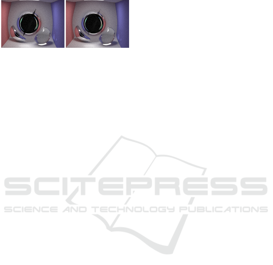
Figure 13: These show the view through the end of an Ellis

wormhole that is inside the room. The wormhole also exerts

strong gravitational forces on its surrounding spacetime and

distorts the geometry of the room. The earth and the satel-

lite from the other side of the wormhole can be seen through

it as crescent shaped disks. The left image has pronounced

error regions at diametrically opposite sides of the worm-

hole’s mouth which are seen as black protrusions. The right

image has been locally smoothed by our renderer in the er-

ror regions.

5.4 Computational Complexity

All the images are rendered on a 2.4 GHz Intel i5

CPU using 4 threads with 1000 samples per pixel.

Here we report the timing to render an image of size

1024 ×768 of a Cornell box, containing a mirror and

a glass sphere, by placing a black or worm hole of size

5 units in the middle of the box. With Schwarzschild

black hole it takes around 80 minutes to render. Ren-

dering time with Kerr black hole ranges from 100

minutes (a/M = 0.1) to 200 minutes (a/M = 0.9).

Due to bidirectional ray tracing and error smoothing

the Ellis wormhole takes longer, nearly 250 minutes.

5.5 Limitations of Our Renderer

Our results are limited somewhat in the complexity of

our scenes, but we do believe we demonstrate the full

range of capabilities that our prototype system cur-

rently has. One major limitation of our renderer is that

it cannot visualize dynamic scenes in curved space-

times, as the animation trajectories of such movement

would also curve (in all four dimensions) that we do

not presently compute. Also of interest may be setting

up space partitioning schemes in curved spacetime to

accelerate such renders.

Also, errors similar to the Ellis wormhole appear

in the images with a Kerr black hole too. We can ap-

ply the same correction to those images as well, which

we have not yet done in the current implementation.

6 CONCLUSION

We present a method to render warped spacetime. We

do this by tracing rays along the null geodesic for

the spacetime, where the spacetime geometry is de-

scribed by its metric. We present a generic ray path

integration scheme that allows us to trace these rays

once the metric has been speciﬁed, and the desired

geodesic equations have been derived. This scheme

allows us to handle ray-object intersections and illu-

mination phenomena while rendering curved space-

time. We show a number of results to validate the out-

put that our renderer is producing, on standard scenes

and cosmological phenomena that have been previ-

ously visualized. Then we render everyday scenes at

terrestrial scales in warped spacetime, around black

holes and wormholes. We believe that these visual-

izations give us a unique understanding of spacetime

in everyday and familiar settings, making it of intrin-

sic pedagogic value. This rendering method is also

very easy to integrate in any path tracer, and there-

fore in existing production pipelines. This also makes

it ideal for producing VFX that are better and more

accurately modelled with real physical basis.

REFERENCES

Bauböck, M., Psaltis, D., Özel, F., and Johannsen, T.

(2012). A Ray-tracing Algorithm for Spinning Com-

pact Object Spacetimes with Arbitrary Quadrupole

Moments. II. Neutron Stars. The Astrophysical Jour-

nal, 753(2):175.

Chan, C.-k., Psaltis, D., and Ozel, F. (2013). GRay: a Mas-

sively Parallel GPU-Based Code for Ray Tracing in

Relativistic Spacetimes. The Astrophysical Journal,

777:13.

Chandrasekhar, S. (2002). The mathematical theory of

black holes. Oxford classic texts in the physical sci-

ences. Oxford Univ. Press, Oxford.

Collier, P. (2013). A Most Incomprehensible Thing: Notes

Towards a Very Gentle Introduction to the Mathemat-

ics of Relativity. Peter Collier.

Ellis, H. G. (1973). Ether ﬂow through a drainhole - a parti-

cle model in general relativity. J. Math. Phys., 14:104–

118.

Fukue, J. and Yokoyama, T. (1988). Color photographs of

an accretion disk around a black hole. Publications of

the Astronomical Society of Japan, 40(1):15–24.

Hamilton, A. (2008). Black hole ﬂight simulator. [Online;

accessed 01-December-2019].

Hartle, J. B. (2003). Gravity: An Introduction to Einstein’s

General Relativity. Benjamin Cummings, illustrate

edition.

James, O., Tunzelmann, E. v., Franklin, P., and Thorne,

K. S. (2015a). Gravitational lensing by spinning black

holes in astrophysics, and in the movie interstellar.

Classical and Quantum Gravity, 32(6):065001.

James, O., von Tunzelmann, E., Franklin, P., and Thorne,

K. S. (2015b). Visualizing interstellar’s wormhole.

American Journal of Physics, 83(6):486–499.

IVAPP 2021 - 12th International Conference on Information Visualization Theory and Applications

Kerr, R. P. (1963). Gravitational ﬁeld of a spinning mass as

an example of algebraically special metrics. Physical

review letters, 11(5):237.

Kuchelmeister, D., Muller, T., Ament, M., Wunner, G., and

Weiskopf, D. (2012). Gpu-based four-dimensional

general-relativistic ray tracing. Computer Physics

Communications, 183(10):2282 – 2290.

Luminet, J. P. (1979). Image of a spherical black hole

with thin accretion disk. Astronomy and Astrophysics,

75:228–235.

Marck, J.-A. (1996). Shortcut method of solution of

geodesic equations for Schwarzschild black hole.

Classical and Quantum Gravity, 13:393–402.

Misner, C., John Archibald Wheeler, C., Misner, U.,

Thorne, K., Wheeler, J., Thorne, U., Freeman, W., and

Company (1973). Gravitation. Number pt. 3 in Grav-

itation. W. H. Freeman.

Morris, M. S. and Thorne, K. S. (1988). Wormholes in

space-time and their use for interstellar travel: A tool

for teaching general relativity. Am. J. Phys., 56:395–

412.

Müller, T. (2014). Geovis—relativistic ray tracing in four-

dimensional spacetimes. Computer Physics Commu-

nications, 185(8):2301 – 2308.

Müller, T. and Boblest, S. (2011). Visualizing circular mo-

tion around a schwarzschild black hole. American

Journal of Physics, 79(1):63–73.

Müller, T., Grottel, S., and Weiskopf, D. (2010). Special

relativistic visualization by local ray tracing. IEEE

Transactions on Visualization and Computer Graph-

ics, 16(6):1243–1250.

Psaltis, D. and Johannsen, T. (2012). A Ray-tracing Algo-

rithm for Spinning Compact Object Spacetimes with

Arbitrary Quadrupole Moments. I. Quasi-Kerr Black

Holes. The Astrophysical Journal, 745(1):1.

Schwarzschild, K. (1916). Über das Gravitationsfeld

eines Massenpunktes nach der Einsteinschen The-

orie. Sitzungsberichte der Königlich Preußischen

Akademie der Wissenschaften (Berlin), 1916, Seite

189-196.

Thorne, K. (2015). The science of interstellar. W. W. Nor-

ton, New York, NY.

Viergutz, S. U. (1993). Image generation in Kerr ge-

ometry. I. Analytical investigations on the station-

ary emitter-observer problem. Astronomy and Astro-

physics, 272:355.

Vincent, F. H., Paumard, T., Gourgoulhon, E., and Per-

rin, G. (2011). GYOTO: a new general relativistic

ray-tracing code. Classical and Quantum Gravity,

28(22):225011.

Weiskopf, D., Schafhitzel, T., and Ertl, T. (2004). Gpu-

based nonlinear ray tracing. Comput. Graph. Forum,

23:625–634.

APPENDIX

Index Notation and the Einstein Summation Con-

vention. In Cartesian coordinates, A vector V con-

sists of a product of its components (V

) and its

basis vectors (ˆe

, ˆe

)

V = V

ˆe

(39)

In index notation, this can be concisely written as V =

. Contravariant vectors (and tensors) are denoted

by an upper index (e.g. V

), while covariant vectors

are denoted by a lower index (e.g. V

Spacetime has four coordinates. It is convention

to use Greek indices (α, β, γ...) to represent them, the

index taking values 0,1, 2, 3 where 0 refers to the time

coordinate and 1,2,3 to the three spatial coordinates.

In Einstein summation convention when an index

occurs twice in the same expression, it means that the

expression is implicitly summed over all possible val-

ues for that index. For Cartesian vectors, the scalar

product A ·B = A

+ A

can be written

in this convention simply as A

. Tensors can have

more than one index. Two tensor X

µν

and Y

being

summed over ν = 0,1, 2, 3 can be written as X

µν

The index ν here is known as a dummy index and the

µ as a free index.

It should be noted that free indices only appear as

either subscript or superscript, never as both and they

must occur exactly once in each term. Dummy in-

dices appear twice in a term, once as subscript and

once as superscript in general four vectors and ten-

sors.

Index labels are themselves not important, and

subject to rules for dummy and free indices. They

can also be arbitrarily renamed in expressions, with-

out loss of meaning.

Non-linear Monte Carlo Ray Tracing for Visualizing Warped Spacetime