
Boosting Self-localization with Graph Convolutional Neural Networks
Takeda Koji and Tanaka Kanji
Department of Engineering, University of Fukui, 3-9-1, Bunkyo, Fukui, Japan
Keywords:
Visual Robot Self-localization, Graph Convolutional Neural Network, Map to DNN.
Abstract:
Scene graph representation has recently merited attention for being flexible and descriptive where visual robot
self-localization is concerned. In a typical self-localization application, the objects, object features and object
relationships of the environment map are projected as nodes, node features and edges, respectively, on to
the scene graph and subsequently mapped to a query scene graph using a graph matching engine. However,
the computational, storage, and communication overhead costs of such a system are directly proportional
to the number of feature dimensionalities of the graph nodes, often significant in large-scale applications.
In this study, we demonstrate the feasibility of a graph convolutional neural network (GCN) to train and
predict alongside a graph matching engine. However, visual features do not often translate well into graph
features in modern graph convolution models, thereby affecting their performance. Therefore, we developed a
novel knowledge transfer framework that introduces an arbitrary self-localization model as the teacher to train
the GCN-based self-localization system i.e., the student. The framework, additionally, facilitated lightweight
storage and communication by formulating the compact output signals from the teacher model as training data.
Results on the Oxford RobotCar datasets reveal that the proposed method outperforms existing comparative
methods and teacher self-localization systems.
1 INTRODUCTION
The graph-based scene model has recently received
significant attention as being a flexible and descrip-
tive scene model for visual robot self-localization.
In self-localization applications, the objects, object
features, and object relationships of the environment
map are generally transposed as nodes, node features,
and edges, respectively, in the scene graph, which
are then matched against a query scene graph by a
graph matching engine; such a scene graph model
can be used with various types of scene data. In
(Gawel et al., 2018), the input scene is segmented
semantically to procure the graph nodes, which are
linked to their neighbours via graph edges. Con-
versely, a view sequence-based localization can be
modelled as a scene graph wherein nodes become the
image frames and the edges connect successive image
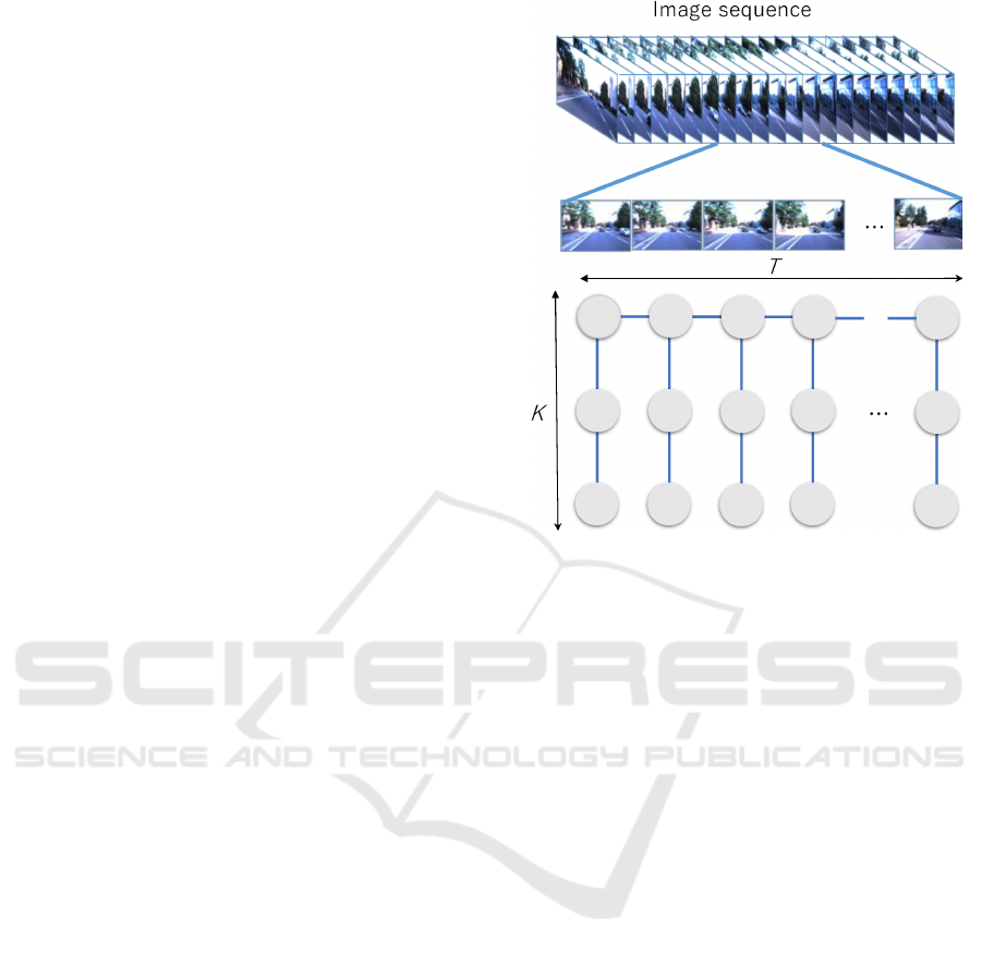
frames (Naseer et al., 2014). For this study, the view
sequence-based scene graph representation, as shown
in Fig. 1, is utilised.
Here, we attempt to analyse the scalability of
a graph-based representation for large-scale applica-
tions such as long-term map-learning (Milford and
Wyeth, 2012). The storage cost of a scene graph is
proportional to the number of dimensionalities of the
graph nodes, i.e., graphs, nodes per graph and dimen-
sionality of the node features, which escalates with
the size of the environment. Moreover, the computa-
tional cost of a graph matching engine is reliant on the
graph size and often requires approximations, such as
dimension-reduction, to achieve considerable compu-
tational speed. To address these issues, we propose a
novel framework to improve the efficiency of a scene
graph-based self-localization system without compro-
mising the accuracy.
In this study, we demonstrate the viability of a
graph-convolutional neural network (GCN), a popu-
lar graph neural network (GNN), as an efficient tool to
train and predict with a graph matching engine (Wang
et al., 2019). In GCN, a graph-convolutional layer
is initially harnessed to extract graph features, which
are then supplied to the graph-summarisation process
to enrich the features. GCN has been successfully ap-
plied to various types of graphical data applications,
including chemical reactivity and web-scale recom-
mender systems (Coley et al., 2019; Ying et al., 2018).
The GCN training and prediction process is computa-
Koji, T. and Kanji, T.
Boosting Self-localization with Graph Convolutional Neural Networks.
DOI: 10.5220/0010212908610868
In Proceedings of the 16th International Joint Conference on Computer Vision, Imaging and Computer Graphics Theory and Applications (VISIGRAPP 2021) - Volume 5: VISAPP, pages
861-868
ISBN: 978-989-758-488-6
Copyright
c
2021 by SCITEPRESS – Science and Technology Publications, Lda. All rights reserved
861
tionally efficient and the complexity is in the order of
O(m + n), where m and n are the edges and nodes re-
spectively.
To assess the performance of a visual robot self-
localization system, it is important to determine how
intuitively the robot converts a given visual feature to
a graph feature. As visual features typically aid in
visual self-localization tasks, such direct conversion
can adversely affect the quality of the resultant graph
features. To this effect, we propose a novel knowl-
edge transfer (KT) framework, which introduces an
arbitrary self-localization model as a teacher to train
the GCN-based self-localization system as the stu-
dent. The proposed framework adopts the standard
KT framework for knowledge distillation, and our
feature learning strategy is inspired by the multimedia
information retrieval (MMIR) domain (Hinton et al.,
2015; Imhof and Braschler, 2018).
The contributions of this study can be summarised
as follows: a) to evaluate the benefits of GCN in not
only augmenting the self-localization performance
but also economising the computational, storage and
communication costs; and b) to conceive a versa-
tile framework for feature learning based on a novel
teacher-to-student KT model. Results on the Ox-
ford RobotCar datasets highlighted the superior per-
formance of the proposed method when compared to
other existing methods and teacher self-localization
systems.
2 RELATED WORK
Robot self-localization using vision is one of the
most important subdomains of mobile robotics and
has been studied in various contexts, including multi-
hypothesis pose tracking, map matching, image re-
trieval and view sequence matching (Himstedt and
Maehle, 2017; Neira et al., 2003; Cummins and New-
man, 2008; Milford and Wyeth, 2012). Our study bor-
rows from view sequence matching, wherein a real-
time short-term view sequence is supplied as a query
to obtain the corresponding component on the map
view sequence.
Unlike previous studies, the proposed approach
models self-localization as a classification problem.
The problem consists of a) partitioning the robot
workspace into different place classes; b) training a
visual place classifier using a class-specific training
set; c) predicting the place class for a given query
image using the pre-trained classifier. For mobile
robotics, training a deep convolutional neural net-
work (DCN) as a visual place classifier is relatively
straightforward. Recently, in (Kim et al., 2019), it
Figure 1: Overview of GCN-based self-localization frame-
work used in conjunction with view-sequence-based scene
graphs; the bottom panel illustrates nodes (circles) and
time/attribute (horizontal/vertical line-segments) edges of a
scene graph.
is successfully implemented for a 3-D point cloud-
based self-localization using scan context image rep-
resentation. However, the current study differs in two
aspects viz. it focuses on the graph-based view se-
quence representation that can accommodate interac-
tions between image frames, and it further addresses
KT from a teacher self-localization model to a student
GCN-based self-localization system.
GNNs have merited interest among the pattern
recognition community as being flexible and efficient
for pattern recognition and machine learning, and
GCN is the most widely used GNN that generalizes
the traditional convolution to data of graph structures.
In the past, GCN has been successfully harnessed in
applications where the traditional DCN proved to be
either inefficient or unsuitable (Coley et al., 2019;
Ying et al., 2018; Zhang and Zhu, 2019). However,
in this study, we revisit a conventional visual robot
self-localization application with the aim to improve
existing solutions.
3 VISUAL SELF-LOCALIZATION
PROBLEM
Here, the self-localization process is modelled as
a classification problem constituting three distinct
VISAPP 2021 - 16th International Conference on Computer Vision Theory and Applications
862
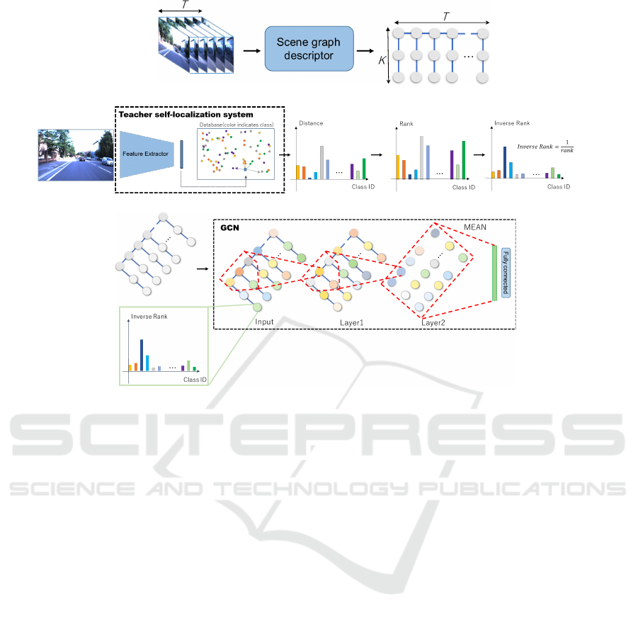
a
b
c
Figure 2: Pipeline of graph matching engine. (a) Scene graph descriptor; (b) KT from teacher self-localization model; and (c)
Supervised learning of the GCN model.
stages: (1) Place partitioning that partitions the robot
workspace into a collection of place classes; (2) Map-
ping (i.e., training) that takes a visual experience with
ground-truth viewpoint information collected in the
workspace as training data and trains a visual place
classifier; (3) Self-localization (i.e., testing) that takes
a query graph representing a short-term live view-
sequence with length T , and predicts the place class.
To reduce storage costs, the trained visual place
classifier is utilised instead of the original train-
ing data during testing. Additionally, the post-
verification techniques like random sample consen-
sus (RANSAC) are omitted to alleviate the overall
computational burden (Raguram et al., 2012). Experi-
mental results nevertheless revealed the robustness of
the proposed framework toward outliers in measure-
ments.
A standard grid-based place partitioning method
is employed to define the place classes. First, a reg-
ular 2-D grid is imposed on the robot workspace i.e.,
a moving plane, and each grid cell is subsequently
viewed as a place class. It should be noted that place
partitioning can be enhanced by adopting pertinent
state-of-the-art techniques.
4 GCN-BASED
SELF-LOCALIZATION
Figure 2 depicts the pipeline of the graph-matching
engine. It consists of three modules, which are de-
tailed in the following.
1. A scene graph descriptor to translate an input view
sequence of length T to a scene graph.
2. A KT module to facilitate communication be-
tween the teacher (arbitrary self-localization
model) and student (GCN-based self-localization
system).
3. A supervised learning module that utilises the
view sequences to train the classifier, which is
used to predict the place class for a given query
sample.
A supervised learning procedure is applied to train
the scene graph classifier. In the mapping stage, a
collection of overlapping sub-sequences of length T
are sampled from the visual experience and divided
into place class-specific training sets according to the
available viewpoint information as well as the pre-
defined place partitioning labels.
Boosting Self-localization with Graph Convolutional Neural Networks
863
We emphasize that all the training set can be
thrown away once the GCN classifier is trained. Con-
sidering the proposed framework employs overlap-
ping sub-sequences as training data, the final dataset
size as well as the number of graph nodes are expected
to be significantly larger than that estimated originally
with the view sequences. Nevertheless, the training
data has no impact on the storage overhead after com-
pressing the training data into a GCN classifier.
The domain invariance is elicited by modifying the
length and intervals of the map/query (for train-
ing/testing respectively) view sequences, as high-
lighted in Fig. 3.
A uniform length T is initially assumed for all
map/query view sequences to develop the invariance
across different domains. Moreover, these T frames
are selected such that the travel distance between
successive frames approximately matches a predeter-
mined value to obtain invariance against the vehi-
cle’s ego-motion speed. This setup is also empiri-
cally corroborated to highlight the efficiency of the
methodology for visual self-localization. It should be
noted that the GCN theory is not limited to homoge-
neous graphs, and extending the proposed approach
to tackle heterogeneous graphs is envisaged in future.
First, a collection of K different image feature ex-
tractors i.e., F
1
, · ··, F
K
, are collated using several
image processing techniques like NetVLAD, Canny
operation, depth regression and semantic segmenta-
tion, as shown in section 4 (Arandjelovi
´
c et al., 2016;
Canny, 1986; Alhashim and Wonka, 2018; Chen
et al., 2018b). Then, each graph node, n = (t, k, f
k
[t]),
represents an attribute feature vector f
k
[t] of the k-th
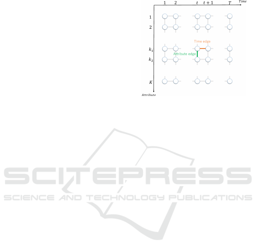
extractor from the tth image frame. Conversely, two
types of graph edges viz. time and attribute, are ap-
plied such that the time edge, e = (t, t + 1, k), con-
nects two graph nodes with successive time indices as
(t, t + 1) with the attribute index k and the attribute
edge, e = (t, k1, k2), connects two graph nodes with
different attribute indices as k
1
and k
2
having the same
time index t.
We now elucidate how a robot can translate input
view images to graph features required for training
and, subsequently, validating the model. A straight-
forward way to achieve this is by directly translat-
ing the visual features, originally designed for visual
self-localization tasks, to graph node features. De-
signing visual features has been a topic of interest in
recent self-localization literature, with past studies al-
ternatively proposing to apply compact, yet discrim-
inative, visual features like autoencoder-based meth-
ods, GAN-based methods, and CNN-based methods
(Merrill and Huang, 2019; Hu et al., 2019; Arand-
jelovi
´
c et al., 2016). In particular, NetVLAD is an
Figure 3: Time and attribute edges.
emerging visual feature extractor in computer vision
and robotics, and hence has been used against the
proposed methodology for comparison (Arandjelovi
´
c
et al., 2016).
One of the main concerns with incorporating
GNNs in this study is that visual features are not op-
timised for graph convolutions. In theory, their su-
perior performances of the past may not necessarily
be replicated in GCN-based self-localization tasks.
Results of our experiments, in fact, showed that the
self-localization performance deteriorated when vi-
sual features were directly used as node features in
the GCN model.
To address this issue, we engage a class-specific
probability distribution vector (PDV) output along
with a teacher self-localization model as the train-
ing data, which is derived from the standard KT
approach for knowledge distillation (Hinton et al.,
2015). The PDV representation facilitates applica-
bility to a broad range of teacher output signals, in-
cluding the tf-idf scores for the bag-of-words im-
age retrieval models, RANSAC scores in the post-
verification stage and mean average intersection-
over-union in object matching systems (Sivic and
Zisserman, 2003; Garcia-Fidalgo and Ortiz, 2018;
S
¨
underhauf et al., 2015).
A node image, I, is converted to a graph feature
vector using a teacher self-localization system, Y , and
an image-to-feature translator, M:
f = M(Y (I)). (1)
The conversion procedure is as follows: a) I is first
supplied to Y to obtain the output PDV signal, o =
Y (I), from the teacher system; and b) o is then
mapped to a graph feature vector as f = M(o).
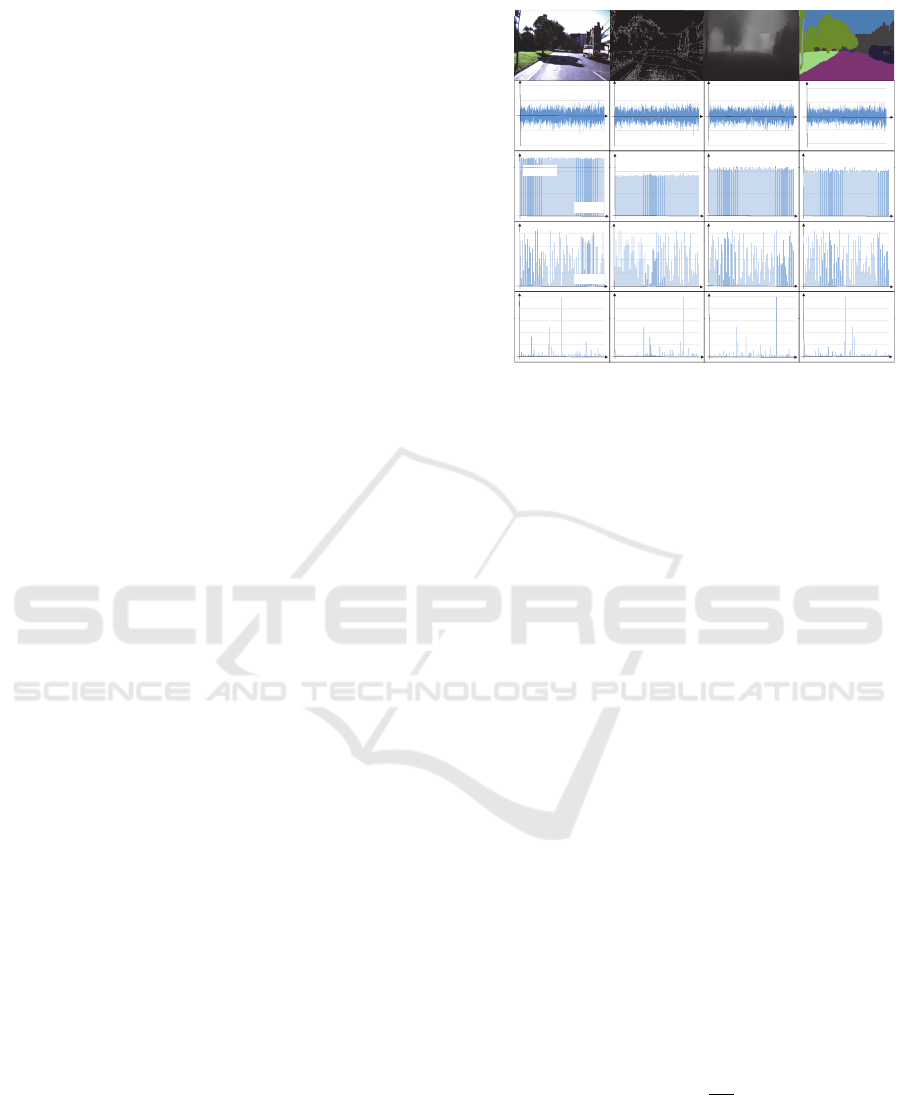
Four teacher systems, Y
1
, Y
2
, Y
3
and Y
4
, were de-
signed for this study, as shown in Fig. 4, by combin-
ing four different image filters, Z
i
(I) (i ∈ [1, 4]), with
VISAPP 2021 - 16th International Conference on Computer Vision Theory and Applications
864
a single nearest-neighbour (NN)-based VLAD match-
ing engine, Y
o
, given by:
Y
i
= Y
o
(Z
i
(I)). (2)
An NN matching engine represents a place class
via a collection of VLAD descriptors that are ex-
tracted from images in the class-specific training set
(Chen et al., 2018a). Then, it computes the image-
to-class distance (i.e., dissimilarity) between a given
query VLAD vector and its nearest neighbour among
the class-specific VLAD vectors.
Four image filters were implemented as depicted
along the horizontal labels in Fig. 4. Z
1
is a basic
identity mapping function, Z
2
represents a Canny im-
age filter that emphasises the gradient of the input im-
age, Z
3
is a depth image regressor trained as an un-
supervised task that predicts a depth image from a
monocular image (Alhashim and Wonka, 2018), and
Z
4
highlights a semantic segmentation filter that con-
verts an input image to a semantic label image whose
pixel colour is derived from the pixel-wise class la-
bels defined in the original colour palette in (Chen
et al., 2018b). Furthermore, four different mapping
functions were applied to the image filters viz. M
1
(·),
M
2
(·), M
3
(·) and M
4
(·) as highlighted along the ver-
tical labels in Fig. 4. M
1
is an identity mapper used
solely with Z
1
. M
2
is a class-specific distance value
vector wherein each c-th place class is assigned the L2
norm of the distance between the query feature and its
nearest neighbour feature in the same class. M
3
em-
ploys a ranking function such that the c-th place class
in a given PDV is assigned a rank by sorting the PDV
elements in the ascending order of their probability
scores and the resultant vector of rank values is used
as the node feature vector; such rank-based represen-
tation was administered based on the recent success
it has found in MMIR applications where ranks are
used as features to fuse information across several do-
mains (for example, the domain of individuals using
MMIR systems) (Imhof and Braschler, 2018). M
4
is
different from M
3
in that the inverse rank values are
exploited instead, which was inspired by the rank fu-
sion approach in (Hsu and Taksa, 2005).
We adopt the standard training procedure for GCN, as
delineated in (Wang et al., 2019), to train the proposed
self-localization system. Initially, a graph is defined
as G = (V, E), where V is the set of nodes and E is
the set of edges. All graphs are undirected i.e., a spe-
cial case of directed graphs where a pair of connected
nodes are indicated by a pair of edges with inverse di-
rections. Let v
i
in V denote a node and e
i j
= (v
i
, v
j
)
in E denote the edge pointing from v
j
to v
i
. Then,
the neighbourhood of node v can then be defined as
N(v) = {u ∈ V | (u, v) ∈ E}. Each node has a corre-
sponding feature vector expressed as h ∈ R
D
. The rep-
Rawimage Canny Depth Semantic
Intensit
y
NetVLAD
Vector
ElementID
y
Match
Distance
ClassID
Distance
Rank
Rank
ClassID
Inverse
Rank
Inverse
Rank
ClassID
Figure 4: Image and feature vectors generated by individual
image filters and image-to-feature translators.
resentation of v is generated by aggregating its own
features h
v
and those in N(v) connected to v via edges,
h
u
(u ∈ N(v)), computed as follows: a) each node ini-
tially receives features from N(v); b) the features are
thereafter summarised in a summation operation; and
c) the summarised features are then supplied to a sin-
gle layer fully-connected neural network, followed by
a non-linear ReLU transformation expressed as:
h
new
i
= ReLU
(
W
(
∑
u∈N(v
i
)∪v
i
h
u
))
, (3)
where W is weight matrix W ∈ R
D×D
′
for applying
the linear transformation, and D and D
′
are the di-
mensions of the feature vector before and after the
operation. The operation at the l-th GCN layer is gen-
eralised as:
h
(l)
i
= ReLU
(
W
(l−1)
(
∑
u∈N(v
i
)∪v
i
h
(l−1)
u
))
. (4)
This operation is applied to all nodes to update the
node features and is repeated L times, corresponding
to the number of layers, which was configured as 2
for this study. Finally, the features of all nodes are
summarised as an average, and then passed to a fully-
connected (FC) and softmax operation given by:
p = Softmax
(
FC
(
1
|V |
∑
u∈V
h
K
u
))
, (5)
where h
u
is the feature at the node u being the output
of the final GCN layer. The system was implemented
using the deep graph library with a Pytorch backend,
as in (Wang et al., 2019).
Boosting Self-localization with Graph Convolutional Neural Networks
865
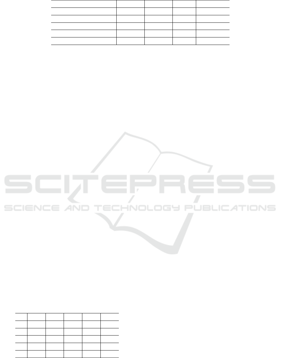
Table 1: Dataset characteristics.
dataset ID weather #images detour roadworks
15-08-28-09-50-22 (A) sun 31,855 × ×
15-10-30-13-52-14 (B) overcast 48,196 × ×
15-11-10-10-32-52 (C) overcast 29,350 × ◦
15-11-12-13-27-51 (D) clouds 41,472 ◦ ◦
15-11-13-10-28-08 (E) overcast 42,968 × ×
5 EXPERIMENTS
We evaluated the proposed methodology on the Ox-
ford RobotCar dataset (Maddern et al., 2017). Table 1
enumerates the characteristics of the dataset. For the
grid-based place partitioning process described in 3,
we used a 14×17 grid with a resolution of 0.1 degree
horizontally and vertically (approximately 110×70
m). Resultantly, the average number of place classes
was 81-86 and a place class was eliminated from the
training and test sets if the number of images belong-
ing to the class was less than or equal to 6. Every
image was cropped to 1080×800 pixels to eliminate
regions occluded by the vehicle itself (i.e., 100 pixels
from each side and 180 pixels from the bottom). The
length of the map and query view sequences was set to
T =10 and the intervals between successive frames in
the travel distance was approximately 2[m]. Finally,
the sequences spanning adjacent places were removed
altogether from both training and test sets. For sim-
plicity, we consider scene graphs with two image fil-
ters (i.e., one attribute edges per image frame) and as
the default setting, the combination of the image fil-
ters with Z
1
and Z
4
is used.
To compare the performance accuracy, we used
the implementation of an NN matching system with
the NetVLAD descriptor (Arandjelovi
´
c et al., 2016)
(adapting the implementation in (Cieslewski et al.,
2018)) which uses the first image frame in each view-
sequence as the query. Conversely, the image-to-class
distance described in 4 was used to measure the class
dissimilarity.
Table 2: Top-1 accuracy.
A B C D E
A 92.3 88.5 80.8 88.4
B 92.4 97.3 87.3 97.6
C 91.5 94.8 90.9 95.7
D 88.2 88.0 93.2 91.6
E 92.7 97.4 99.2 94.4
The number of GCN layers was set to 2 and fea-
ture dimensionality of the GCN layers was configured
as C, 256, 256, and C for a size C class set. For
node summarisation, the SUM and ReLU operations
were administered. The number of epochs, batch
size and learning rate were set to 5, 32, and 0.001,
respectively. The training was conducted for 170 s
on 31,835 samples on a personal computer running
the Intel(R) Xeon(R) GOLC 6130 CPU at 2.10 GHz.
The self-localization performance was measured by
the top-1 accuracy, as highlighted in Table 4. The
horizontal and vertical indexes in the table are IDs
of query and map datasets, respectively. The predic-
tion turnaround time amounted to 15.5 ms per query
graph, rendering the proposed framework as compu-
tationally expeditious. This implies significant reduc-
tion in computational complexity compared with pre-
vious approaches such as graph matching.
Table 4 shows results for the proposed method
with different choices of the image filter Z
i
as well
as the comparing method. From top to bottom, the
1st, 2nd and 3rd lines correspond to the combinations
of image filters (Z
1
, Z
2
), (Z
1
, Z
3
) and (Z
1
, Z
4
), while
the 4th line corresponds the result with the comparing
method. By comparing the different combinations of
image filters, the combination of Z
1
and Z
4
yielded
the best performance. It can be seen that the pro-
posed method outperforms the comparing method for
almost all settings considered here.
Table 4 enumerates the comparative results of ad-
ministering different combinations of image filters on
the proposed method against existing methods. From
top to bottom, each line corresponds to that image
filters Z
1
, Z
2
, Z
3
and Z
4
. Among the various com-
binations applied, that of Z
1
and Z
4
yielded the best
outcome. It can be seen that the proposed method
surpassed its competitors in most of the settings con-
sidered here.
Two experiments were performed as part of an ab-
lation study. In the first instance, the scene graphs
were modified by removing the edges to train the
model and, in the second, the graph topology was
modified by removing one of the time and attribute
edges at random. Table Table 3 outlines the exper-
imental results. It is apparent that graphs with both
time and attribute edges worked significantly better
in almost all cases. The use of attribute edges fa-
VISAPP 2021 - 16th International Conference on Computer Vision Theory and Applications
866
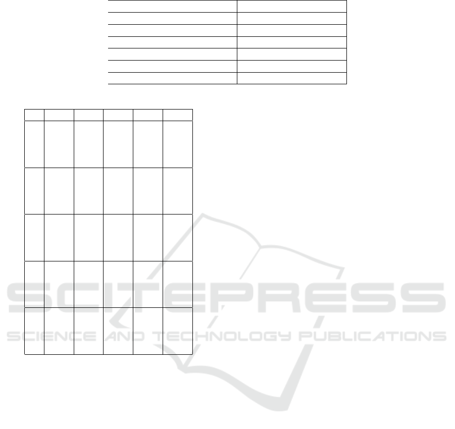
Table 3: Performance comparison.
Method Average Top-1 accuracy
Ours 92.3
NetVLAD 87.9
Ours w/o edge 89.0
Ours w/o attribute edge 91.5
Ours w/o time edge 88.7
Ours w/o attribute node/edge 91.7
Table 4: Results for different choices of image filters.
A B C D E
A
92.3
92.8
93.2
83.1
88.5
90.0
89.9
85.0
80.8
82.0
83.3
79.7
88.4
90.2
91.5
82.2
B
92.4
92.3
91.1
86.9
97.3
98.5
96.7
95.2
86.6
85.0
84.2
81.6
97.8
97.6
97.6
95.5
C
91.5
91.2
91.7
83.6
94.8
94.9
94.7
91.7
90.9
89.8
90.7
88.7
95.7
95.8
95.8
94.0
D
88.2
87.6
87.2
78.0
88.0
87.7
87.3
87.1
93.2
87.6
93.2
92.4
91.6
91.9
92.6
88.4
E
92.7
93.3
94.5
83.9
97.4
97.4
96.9
93.3
99.2
99.0
99.2
97.3
94.4
93.1
94.1
91.1
cilitated resistance against feature ambiguity by com-
pensating individual features’ drawbacks. The use of
time edges facilitated resistance against partial occlu-
sions incurred from changes in illumination between
the training and test domains. Consequently, the pro-
posed framework showed potential to solve a variety
of problems by integrating the available cues from
different image filters as well as the time and spatial
graphs.
6 CONCLUSIONS
We investigated the utility of a GCN model to aug-
ment the performance of visual robot self-localization
systems whilst alleviating the computational, stor-
age and communication costs. Furthermore, a novel
and versatile KT framework was conceived to fa-
cilitate information transfer from an arbitrary self-
localization model (teacher) that integrated the avail-
able cues from different image filters as well as the
time and spatial contextual information. Results on
the Oxford RobotCar datasets substantiated the ro-
bustness of the proposed framework when compared
to other existing methods and teacher self-localization
systems. Although we harnessed a view sequence-
based scene graph representation for this study, other
scene graph representations can also be employed, in-
cluding attribute grammar-based scene graphs (Stein-
lechner et al., 2019). We attempt to explore other
general heterogeneous scene graphs so as to tackle
map/query scene graphs of variable sizes and shapes
in future.
ACKNOWLEDGEMENTS
Our work has been supported in part by JSPS
KAKENHI Grant-in-Aid for Scientific Research (C)
17K00361, and (C) 20K12008.
REFERENCES
Alhashim, I. and Wonka, P. (2018). High quality monoc-
ular depth estimation via transfer learning. CoRR,
abs/1812.11941.
Arandjelovi
´
c, R., Gronat, P., Torii, A., Pajdla, T., and Sivic,
J. (2016). NetVLAD: CNN architecture for weakly
supervised place recognition. In IEEE Conference on
Computer Vision and Pattern Recognition.
Canny, J. (1986). A computational approach to edge de-
tection. IEEE Transactions on pattern analysis and
machine intelligence
, (6):679–698.
Chen, G. H., Shah, D., et al. (2018a). Explaining the suc-
cess of nearest neighbor methods in prediction. Now
Publishers.
Chen, L., Zhu, Y., Papandreou, G., Schroff, F., and Adam,
H. (2018b). Encoder-decoder with atrous separable
convolution for semantic image segmentation. In Fer-
rari, V., Hebert, M., Sminchisescu, C., and Weiss, Y.,
editors, Computer Vision - ECCV 2018 - 15th Euro-
pean Conference, Munich, Germany, September 8-14,
2018, Proceedings, Part VII, volume 11211 of Lecture
Notes in Computer Science, pages 833–851. Springer.
Cieslewski, T., Choudhary, S., and Scaramuzza, D. (2018).
Data-efficient decentralized visual SLAM. In 2018
IEEE International Conference on Robotics and Au-
tomation, ICRA, pages 2466–2473.
Boosting Self-localization with Graph Convolutional Neural Networks
867

Coley, C. W., Jin, W., Rogers, L., Jamison, T. F., Jaakkola,
T. S., Green, W. H., Barzilay, R., and Jensen, K. F.
(2019). A graph-convolutional neural network model
for the prediction of chemical reactivity. Chemical
science, 10(2):370–377.
Cummins, M. and Newman, P. (2008). Fab-map: Proba-
bilistic localization and mapping in the space of ap-
pearance. Int. J. Robotics Research, 27(6):647–665.
Garcia-Fidalgo, E. and Ortiz, A. (2018). ibow-lcd: An
appearance-based loop-closure detection approach us-
ing incremental bags of binary words. IEEE Robotics
and Automation Letters, 3(4):3051–3057.
Gawel, A., Del Don, C., Siegwart, R., Nieto, J., and Cadena,
C. (2018). X-view: Graph-based semantic multi-view
localization. IEEE Robotics and Automation Letters,
3(3):1687–1694.
Himstedt, M. and Maehle, E. (2017). Semantic monte-
carlo localization in changing environments using rgb-
d cameras. In 2017 European Conference on Mobile
Robots (ECMR), pages 1–8. IEEE.
Hinton, G., Vinyals, O., and Dean, J. (2015). Distilling
the knowledge in a neural network. arXiv preprint
arXiv:1503.02531.
Hsu, D. F. and Taksa, I. (2005). Comparing rank and score
combination methods for data fusion in information
retrieval. Information retrieval, 8(3):449–480.
Hu, H., Wang, H., Liu, Z., Yang, C., Chen, W., and
Xie, L. (2019). Retrieval-based localization based on
domain-invariant feature learning under changing en-
vironments. In IEEE/RSJ Int. Conf. Intelligent Robots
and Systems (IROS), pages 3684–3689.
Imhof, M. and Braschler, M. (2018). A study of untrained
models for multimodal information retrieval. Infor-
mation Retrieval Journal, 21(1):81–106.
Kim, G., Park, B., and Kim, A. (2019). 1-day learning, 1-
year localization: Long-term lidar localization using
scan context image. IEEE Robotics and Automation
Letters, 4(2):1948–1955.
Maddern, W., Pascoe, G., Linegar, C., and Newman, P.
(2017). 1 Year, 1000km: The Oxford RobotCar
Dataset. The International Journal of Robotics Re-
search (IJRR), 36(1):3–15.
Merrill, N. and Huang, G. (2019). CALC2.0: Com-
bining appearance, semantic and geometric informa-
tion for robust and efficient visual loop closure. In
IEEE/RSJ Int. Conf. Intelligent Robots and Systems
(IROS), Macau, China.
Milford, M. J. and Wyeth, G. F. (2012). Seqslam: Vi-
sual route-based navigation for sunny summer days
and stormy winter nights. In 2012 IEEE Int. Conf.
Robotics and Automation, pages 1643–1649. IEEE.
Naseer, T., Spinello, L., Burgard, W., and Stachniss, C.
(2014). Robust visual robot localization across sea-
sons using network flows. In AAAI, pages 2564–2570.
Neira, J., Tard
´
os, J. D., and Castellanos, J. A. (2003). Linear
time vehicle relocation in slam. In ICRA, pages 427–
433. Citeseer.
Raguram, R., Chum, O., Pollefeys, M., Matas, J., and
Frahm, J.-M. (2012). Usac: a universal framework for
random sample consensus. IEEE transactions on pat-
tern analysis and machine intelligence, 35(8):2022–
2038.
Sivic, J. and Zisserman, A. (2003). Video google: A text
retrieval approach to object matching in videos. In
null, page 1470.
Steinlechner, H., Haaser, G., Maierhofer, S., and Tobler,
R. F. (2019). Attribute grammars for incremental
scene graph rendering. In VISIGRAPP (1: GRAPP),
pages 77–88.
S
¨
underhauf, N., Shirazi, S., Dayoub, F., Upcroft, B., and
Milford, M. (2015). On the performance of convnet
features for place recognition. In IEEE/RSJ Int. Conf.
Intelligent Robots and Systems (IROS), pages 4297–
4304.
Wang, M., Yu, L., Zheng, D., Gan, Q., Gai, Y., Ye, Z., Li,
M., Zhou, J., Huang, Q., Ma, C., Huang, Z., Guo, Q.,
Zhang, H., Lin, H., Zhao, J., Li, J., Smola, A. J., and
Zhang, Z. (2019). Deep graph library: Towards ef-
ficient and scalable deep learning on graphs. ICLR
Workshop on Representation Learning on Graphs and
Manifolds.
Ying, R., He, R., Chen, K., Eksombatchai, P., Hamilton,
W. L., and Leskovec, J. (2018). Graph convolutional
neural networks for web-scale recommender systems.
In Proceedings of the 24th ACM SIGKDD Int. Conf.
Knowledge Discovery & Data Mining, pages 974–
983.
Zhang, L. and Zhu, Z. (2019). Unsupervised feature learn-
ing for point cloud understanding by contrasting and
clustering using graph convolutional neural networks.
In IEEE Int. Conf. 3D Vision, pages 395–404.
VISAPP 2021 - 16th International Conference on Computer Vision Theory and Applications
868
