Vertex Climax: Converting Geometry into a Non-nanifold Midsurface

Christoph Schinko

1,2

and Torsten Ullrich

1,2 a

Fraunhofer Austria Research GmbH, Graz, Austria

Technische Universit

at Graz, Graz, Austria

Keywords:

Midsurface, Grid-based Algorithm, Volume Graphics, Design Automation.

Abstract:

The physical simulation of CAD models is usually performed using the ﬁnite elements method (FEM). If the

input CAD model has one dimension that is signiﬁcantly smaller than its other dimensions, it is possible to

perform the physical simulation using thin shells only. While thin shells offer an enormous speed-up in any

simulation, the conversion of an arbitrary CAD model into a thin shell representation is extremely difﬁcult

due to its non-uniqueness and its dependence on the simulation method used afterwards. The current state-of-

the-art algorithms in conversion voxelize the input geometry and remove voxels based on matched, predeﬁned

local neighborhood conﬁgurations until only one layer of voxels remains.

In this article we discuss a new approach that can extract a midsurface of a thin solid using a kernel-based

approach: In contrast to other voxel-based thinning approaches, our algorithm applies a kernel onto a binary

grid. In the resulting density ﬁeld, opposing surface-voxels are iteratively moved towards each other until a

thin representation is obtained.

1 INTRODUCTION

The analysis of thin-walled parts is a discipline of

Computer-Aided Engineering (CAE) analysis. As

physical simulations are computationally costly, they

beneﬁt from reduced-complexity representations, so

called “Midsurfaces” (Kulkarni, 2016). The reduc-

tion in complexity is achieved by replacing such

Computer-Aided Design (CAD) models with a sim-

pliﬁed model consisting of non-manifold 2D-surfaces

lying (mostly) midway of the original walls.

Midsurfaces are part of the larger family of me-

dial objects. A common member of this family is the

medial axis.

Deﬁnition: The medial axis (also called medial sur-

face) of a closed object is the set of centers of empty

spheres which touch the surface of the object at more

than one point.

Another member of the family of medial objects

is the straight skeleton. The straight skeleton is de-

ﬁned only for polygons and has been introduced by O.

AICHHOLZER and F. AURENHAMMER (Aichholzer

and Aurenhammer, 1996). In contrast to the medial

axis it consists only of line segments (see Figure 1).

The straight skeleton is deﬁned by a shrinking pro-

cess of the polygon. The edges of the polygon are

https://orcid.org/0000-0002-7866-9762

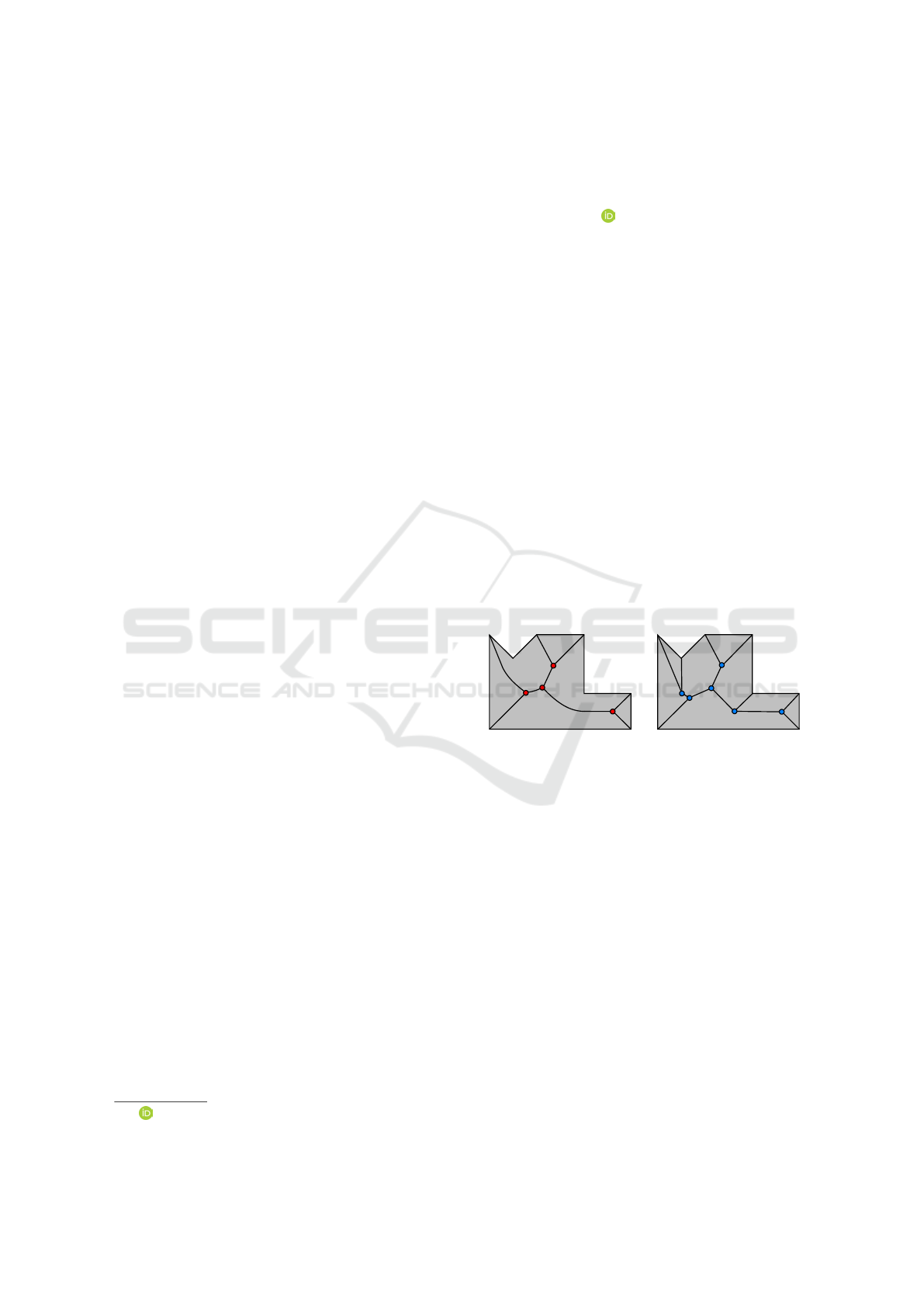
Figure 1: The medial axis of some input geometry consists

of all points that are the center of a sphere which touches the

input at more than one point (left). The straight skeleton is

the result of a shrinking process returning a graph structure

of line segments only (right).

moved inwards in a self-parallel manner and at the

same speed. When all parts have shrunken to zero, the

process terminates. The straight skeleton now con-

sists of the paths drawn by the polygon vertices during

the shrinking process. The result can be seen as a vari-

ant of the medial axis, because, in the case of convex

polygons, both structures are identical (Demuth and

Aurenhammer, 2010).

Both, the deﬁnition of a medial axis as well as the

deﬁnition of the straight skeleton, only depend on the

input object. By contrast, the midsurface deﬁnition

not only depends on the input, but also on the output

of a subsequent analysis:

Deﬁnition: The midsurface of a closed, thin-walled

object is a set of non-manifold surfaces which re-

veal in a CAE analysis the same results (within a δ-

Schinko, C. and Ullrich, T.

Vertex Climax: Converting Geometry into a Non-nanifold Midsurface.

DOI: 10.5220/0010210401850192

In Proceedings of the 16th International Joint Conference on Computer Vision, Imaging and Computer Graphics Theory and Applications (VISIGRAPP 2021) - Volume 1: GRAPP, pages

185-192

ISBN: 978-989-758-488-6

185

tolerance) as the closed, thin-walled input model.

Therefore, any statements regarding the correct-

ness of a midsurface transformation can only be vali-

dated within a speciﬁc context. A possible difference

between the results of both transformation types is il-

lustrated in 2D in Figure 2.

Figure 2: The result of a medial axis transformation (left)

and the midsurface transformation of a thin-walled part

(grey) are usually different. As the midsurface has to re-

spect follow-up simulation usages, both results (left & right)

may be a correct midsurface depending on the application

context.

This article presents a novel voxel-based midsur-

face generation approach for thin-walled objects; the

ﬁrst, preliminary sketch of this algorithm has been

presented in a poster session at the Fabrication &

Sculpting Event (FASE) at Shape Modeling Interna-

tional (SMI) 2020 (Schinko and Ullrich, 2020). In

contrast to the preliminary sketch, a detailed descrip-

tion and a thorough evaluation have been added to this

article.

2 RELATED WORK

Related work in the area of midsurface generation for

solid geometries can be divided into surface-based

approaches and grid-based (so-called thinning) ap-

proaches.

H. LOCKETT and M. GUENOV address the difﬁ-

culty in ﬁnding similarity measures for evaluating the

quality of midsurface models (Lockett and Guenov,

2008). Without a ground truth, the proposed meth-

ods perform a geometric and topological comparison

between the midsurface models and their solid coun-

terparts. A global measure of geometric similarity is

based on the Hausdorff distance (Ullrich et al., 2008)

and deﬁnes the proportion of solid model points that

are within a speciﬁed threshold distance of the mid-

surface model. For measuring the global topological

similarity, geometry graph attributes are used. Both

measures can be combined into an overall similarity

index to provide interesting insights.

2.1 Top-down

The group of top-down approaches are surface-

based approaches working on boundary representa-

tions (Schinko et al., 2017). A divide and conquer

strategy simpliﬁes the transformation into midsur-

faces by splitting complex parts into smaller sub-parts

according to semantic interrelationships (Sun et al.,

2016). This kind of approach is also used by Y.

H. WOO and C. U. CHOO (Woo and Choo, 2009).

They decompose a solid model into simple volumes

and generate midsurfaces using an existing algorithm

based on face-pairs (the top and the bottom side of

a thin layer are called face-pairs or corresponding

faces (Rezayat, 1996); in a boundary representation

these faces usually don’t have any explicit correspon-

dence).

In their work, NOLAN et al. rely on feature detec-

tion to assign mixed-dimensional ﬁnite element mod-

els to three categories: complex regions, long-slender

regions, and thin-sheet regions (Nolan et al., 2014).

Relations between the original solid model and the

dimensionally reduced version are maintained.

In the area of surface-based midsurface genera-

tion, the state-of-the-art approaches for decomposi-

tion (Kulkarni et al., 2017b), identiﬁcation of cor-

responding faces (Kulkarni and Kale, 2014), and a

divide and conquer strategy (Kulkarni et al., 2017a)

have been presented by Y. H. KULKARNI: “Develop-

ment of Algorithms for Generating Connected Mid-

surfaces using Feature Information in Thin-Walled

Parts” (Kulkarni, 2016).

2.2 Bottom-up

Due to the nature of our approach being grid-based,

this Section focuses on a subgroup of so-called thin-

ning approaches. The idea behind these approaches

is to iteratively shrink an object locally by offset-

ting its boundary towards its interior. This process is

stopped, when the interior vanishes and just a (usu-

ally non-manifold) surface structure remains. Like

our approach, many thinning approaches work on bi-

nary voxels, a concept attributed to the ﬁeld of digital

topology. Early work in this ﬁeld dates back to the late

1960s and is surveyed by T.Y KONG and A. ROSEN-

FELD (Kong and Rosenfeld, 1989). A good descrip-

tion of toplogical structures of voxels and concepts

like neighborhood, connectivity and Euler number is

given by J. TORIWAKI and T. YONEKURA (Toriwaki

and Yonekura, 2002). Their work also introduces new

local features to study the effect of deleting 1-voxels

– a fundamental process during thinning.

Thinning approaches have a long history: P.

KWOK and V. RANJAN give a good overview of the

most important thinning algorithms up to 1991 (Kwok

and Ranjan, 1991). All presented algorithms work on

voxel data and eventually result in a skeleton rather

than a surface. Another volume thinning method for

generating a skeleton that can be used in searching

for intersected cells in isosurface propagation is pre-

GRAPP 2021 - 16th International Conference on Computer Graphics Theory and Applications

186

sented by ITOH et al. (Itoh et al., 1996). Their graph-

based approach connects all extremum points of a vol-

ume to a one-cell wide skeleton and contains its topo-

logical features. S. PROHASKA and H.-C. HEGE pro-

pose a robust, noise resistant criterion for the charac-

terization of plane-like skeletons (Prohaska and Hege,

2002). Their algorithm uses the geodesic distance

along the object’s boundary and a distance map. After

obtaining a skeleton of lines and surfaces, the focus is

on obtaining a surface representation for expressive

rendering of complex structures.

In contrast to the already mentioned algorithms

that return skeletons, the work by T.-C. LEE and

R. L. KASHYAP on thinning algorithms is con-

cerned with parallel thinning for extracting medial

surfaces and medial axes of binary voxel data (Lee

and Kashyap, 1994). The algorithm uses the Euler

characteristic to preserve topological properties of bi-

nary voxel data during the thinning process. Another

thinning algorithm for extracting medial surfaces is

presented by C.-M. MA and S.-Y. WAN (Ma and

Wan, 2001). It deﬁnes two sets of voxels on the

grid: one consisting of the 26-neighborhood of all 1-

voxels and one consisting of the 6-neighborhood of

all 0-voxels. The algorithm alternatively works on

the two sets deleting all possible 1-voxels, and ter-

minates when no 1-voxels can be deleted anymore. It

is proven to preserve connectivity.

The work of FUJIMORI et al. focuses on extract-

ing separated medial surfaces (Fujimori et al., 2006).

Medial surfaces are obtained by classifying voxels

into medial surface voxels using geodesic distances

along all three axes. Connected regions are separated

by using the average thickness as an indicator (a con-

stant thickness of all parts is assumed). The separa-

tion is performed by offsetting them into the direc-

tion of the object surface. In a ﬁnal step, a polygo-

nal surface is extracted using a marching cubes ap-

proach. Another thinning approach for medial sur-

face extraction is presented by K. PAL

AGYI and G.

EMETH (Pal

agyi and N

emeth, 2009). The proposed

algorithms rely on sufﬁcient conditions for parallel,

topology-preserving reduction operators. A novel

thinning scheme using iteration-level endpoint check-

ing is proposed in follow-up work (N

emeth et al.,

2010).

2.3 Surface Reconstruction

Using a grid-based data structure for thinning, our

approach has to convert the remaining voxels rep-

resenting the midsurface into a polygonal, non-

manifold representation. An important algorithm to

extract a polygonal representation of an isosurface

within a three-dimensional, discrete scalar ﬁeld is

the well-known marching cubes algorithm by W. E.

LORENSEN and H. E. CLINE (Lorensen and Cline,

1987). It is in the nature of the marching cubes al-

gorithm to produce a dense triangulation (even on

ﬂat surfaces) and voxel artifacts. In case normal

information is available for each voxel, surface re-

construction algorithms are able to produce a much

smoother mesh (Ju et al., 2002). Another approach

is presented by KAZHDAN et al. showing that sur-

face reconstruction of Hermite data can be formu-

lated as a Poisson problem (Kazhdan et al., 2006).

The algorithm reconstructs a watertight triangulation

of the surface of a model.While all these algorithms

produce a closed surface for all connected regions

of voxels, they are not suitable for midsurface re-

construction due to its non-manifold nature (without

volume and orientation). Q. T. NGUYEN and A.

J. P. GOMES propose an algorithm for triangulating

non-manifold implicit surfaces (Nguyen and Gomes,

2016). The idea is to leverage data generated by

marching cubes and to “heal” the triangulation inside

so-called critical cubes. Additional work on polygo-

nizing non-manifold implicit surfaces is presented by

YAMAZAKI et al. (Yamzaki et al., 2002). By allow-

ing discontinuity of the ﬁeld function, the proposed

method yields a non-manifold surface exhibiting fea-

tures like holes and boundaries. Another approach to

reconstruct medial surfaces from volumetric data of

thin-plate objects is presented by T. MICHIKAWA and

H. SUZUKI (Michikawa and Suzuki, 2010). Their al-

gorithm is based on distance ﬁelds of binary volumes

and uses spherical support to build correct junctions

where conventional approaches produce small cavi-

ties.

As the result of all midsurface generation algo-

rithms require manual inspection and corrections, the

manual and the automatic creation of a midsurface

still cause a similar effort.

3 VERTEX CLIMAX

Our new grid-based approach consists of four steps,

which are described shortly to give an overview, and

which are illustrated in the Figures 3 and 4. The ﬁrst

step builds a binary 3D grid (see Figure 3, left) and

marks each voxel (light red) that contains some part

of the input surface geometry (dark red).

The second step interprets the binary grid as a den-

sity ﬁeld with the previous markup as initial 0.0 resp.

1.0 values and applies a kernel Σ to it. In Figure 3

(right) the kernel is a simple counter (light red) that

sums the values of each 3 × 3 neighborhood N

. The

Vertex Climax: Converting Geometry into a Non-nanifold Midsurface

187

illustration shows the color-coded result.

number of

1-voxels in N

1234567

Figure 3: The new “vertex climax” algorithm determines

the midsurface of a geometric model. In the ﬁrst step (left)

the input surface geometry is rasterized into a voxel rep-

resentation. Having rasterized the input surface geometry

in binary voxels, an accumulation kernel Σ transforms the

binary voxels into a density ﬁeld (right).

In the third step (see Figure 4, left), the vertices

of the original input data are moved within the den-

sity ﬁeld towards the climax (black arrows in the color

coded grid).

Finally, vertices which approach each other are

clustered and merged (see grey circles in Figure 4).

Having merged all clusters of vertices, the resulting

two-sided, incident surfaces are merged to one-sided

surfaces. The result is a midsurface.

Figure 4: The accumulated density ﬁeld deﬁnes a direction:

The vertices of the input surface geometry are moved to-

wards the density climax (left). The merge step (right) is

performed by a mean-shift clustering algorithm (illustrated

by grey circles). While merging the vertices, the surfaces

(top and bottom of a geometry; dotted lines) merge as well

(black line).

3.1 Rasterization Step

The Vertex Climax algorithm can be applied to trian-

gle meshes only. This prerequisite is not a limitation

as most CAD systems offer the possibility to export

the tessellated geometry.Besides the tessellated ge-

ometry the algorithm needs two additional values: ε

and δ, which are the smallest / greatest distance be-

tween two opposite surfaces that should be merged to

one midsurface. All other subsequent parameters (see

Table 2) are set automatically and do not need to be

modiﬁed.

The ﬁrst step builds a binary 3D grid and marks

each voxel that has a non-empty intersection with the

input surface geometry (Ogayar-Anguita et al., 2020).

If the grid size α, i.e. the edge length of each cube in

the voxel grid, is not speciﬁed, the algorithm uses the

default value α =

ε.

3.2 Voxel Kernel

The second step interprets the binary grid as a density

ﬁeld with the values 0.0, if a voxel does not contain

any geometry, and 1.0 otherwise. The main idea of

the second step is to spread the density values using

a kernel. The overlaps of the kernels at the position

of the midsurface result in signiﬁcantly higher values

compared to their neighborhood.

The vertex climax uses a uniform distribution over

a 3D sphere with radius κ. The implementation sim-

ply sums for each voxel (i, j, k) the values of all sur-

rounding voxels (r, s, t) with an Euclidean distance

less than κ between the voxels’ centers. Although

many computer vision algorithms use other metrics,

the Euclidean distance was chosen because it best cor-

responds to the approach of a manual midsurface con-

struction, which is the blueprint for this algorithm.

3.3 Vertex Climax

In the third step, the vertices of the original input tes-

sellation data are moved within the density ﬁeld gen-

erated in the previous steps. The start position of a

moving vertex is the center of its corresponding voxel.

Then each vertex moves to the center of a neighboring

voxel with the highest density until

1. no improvement concerning density values is pos-

sible or

2. the length of the movement path exceeds the

greatest distance δ between two opposite surfaces

that should be merged to one midsurface.

3.4 Vertex Clustering & Topological

Cleaning

Having moved all vertices, the resulting set of vertices

is clustered using a mean-shift clustering algorithm

with a window size ω (with default value δ). The re-

sult is already a two-sided midsurface, in which each

part is represented by two incident surfaces. As a one-

sided midsurface representation is desired (the goal

is as little geometry as possible), a dense resampling

of the two-sided midsurface and a reconstruction ac-

cording to SHAWN and WATSON (Shawn and Watson,

2011) returns the desired result.

GRAPP 2021 - 16th International Conference on Computer Graphics Theory and Applications

188

4 EVALUATION

In order to evaluate the “Vertex Climax” algorithm,

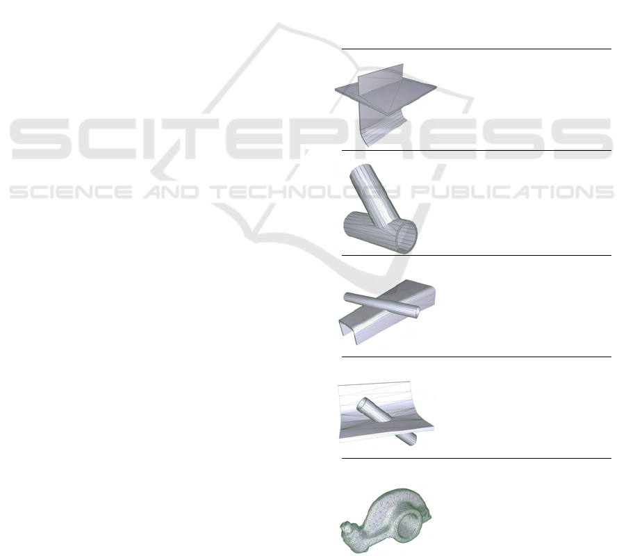
we created ﬁve geometric conﬁgurations and applied

the new algorithm to them. The ﬁrst data set consists

of two penetrating sheet metal parts of different size

and thickness, one of which is bent at one end. The

second data set consists of two pipes with different

diameters and wall thicknesses. The arrangement is

an acute-angled T-construction where the pipe with

the larger diameter is continuous. The third data set

consists of a widening U-shaped beam connected to a

pipe at a top outlet. The fourth conﬁguration consists

of a bent sheet metal on which two pipes are aligned

at acute angles, i.e. the sheet metal is not penetrated

and the pipes are not continuous. The last data set is

a laser-scanned part which contains noise and which

does not meet the thin-solid requirements.

Table 1 illustrates each input data set and lists their

geometric properties; i.e. the number of triangles, the

size of the axis-aligned bounding box ∆ AABB, the

smallest distance ε and the greatest distance δ be-

tween two opposite surfaces that should be merged

to one midsurface. Please note, that the last data set

is not a thin solid. The measured values ε and δ refer

only to the parts that fulﬁll the thin-solid condition.

All evaluations of the “Vertex Climax” algorithm

use the heuristics of the default values (see Table 2).

No additional adjustment has been made. As a con-

sequence, having measured the geometric sizes ε and

δ, the algorithm runs fully automatically and requires

no user interaction.

4.1 Intermediate Steps

For thin-solid input geometry, vertex climax and ver-

tex clustering are the most time consuming steps (see

Table 3). When the thin-solid condition is violated

and a signiﬁcant amount of grid cells is occupied, the

accumulation step contributes most to the overall run-

time of the algorithm.

Using the default values for the grid size, the re-

sulting grids vary between 0.2 × 10

cells and 50.7 ×

cells (for data set #2 and #3, respectively). Of all

data sets, between 0.1 × 10

and 12.6 × 10

cells are

occupied; i.e. between 19% upto 55% of all cells are

nonempty.

Figure 5 shows some intermediate results of the

rasterization and the subsequently applied kernel. In

order to have a better view on the results of the kernel,

each cell is rendered as a cube that is smaller than the

cell size; additionally, the volume is clipped in the

middle.

4.2 Geometric Distance

The vertex movement within the density ﬁeld is lim-

ited by a maximum path length, which is the great-

est thickness δ. In combination with the mean-

shift-clustering, which is limited by the window size

ω, the Hausdorff distance (Ullrich et al., 2008) be-

tween the input surface geometry and the result-

ing midsurface is expected to be at the same level.

In the geometric analysis listed in Table 4, the

vertex movement including vertex clustering corre-

sponds to the one-sided distance of an actual-target-

comparison (Schinko et al., 2011). Its values (aver-

age ± standard-deviation per vertex) should be ap-

Table 1: The input data sets represent geometric conﬁgura-

tions commonly used in computer-aided geometric design.

Please note that in contrast to the data sets #1 – #4, the data

set #5 is not a thin solid. It has been included to demonstrate

limitations.

data set statistics

data set #1

# elements 84 triangles

AABB

∆ x 149.416

∆ y 174.837

∆ z 155.954

ε 1.77

δ 4.84

data set #2

# elements 360 triangles

AABB

∆ x 63.6580

∆ y 167.720

∆ z 172.135

ε 4.46

δ 5.22

data set #3

# elements 524 triangles

AABB

∆ x 263.307

∆ y 76.1719

∆ z 212.861

ε 0.98

δ 5.65

data set #4

# elements 388 triangles

AABB

∆ x 139.035

∆ y 158.949

∆ z 123.290

ε 1.51

δ 6.90

data set #5

# elements 20088 triangles

AABB

∆ x 2.38100

∆ y 4.04000

∆ z 7.84600

ε 0.35

δ [ 0.60 ] (thin

solid parts only)

Vertex Climax: Converting Geometry into a Non-nanifold Midsurface

189

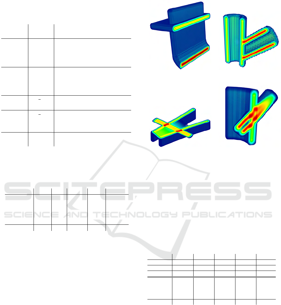
Table 2: The default parameter settings of the vertex climax

algorithm do not need to be modiﬁed in most application

cases.

param- default semantic

eter value

ε – smallest thickness; i.e. the

smallest distance between two

opposite surfaces that should be

merged to one midsurface

δ – greatest thickness; i.e. the

greatest distance between two

opposite surfaces that should be

merged to one midsurface

ε grid size; i.e. the edge length of

each cube in the voxel grid

δ kernel radius; i.e. the support

radius of the uniform, spherical

kernel

ω δ window size of the mean shift

clustering algorithm

Table 3: The algorithm consists of four steps (rasterization,

accumulation, vertex climax and vertex clustering). For

thin-solid input data sets, vertex climax and vertex cluster-

ing are the most resource demanding steps of the algoritm.

data set #1 #2 #3 #4 #5

runtime [s]

step

0.01 0.01 0.01 0.01 23.20

step

#2 0.01 0.01 0.01 0.01 2226.83

step #3

16.84 1.04 162.70 27.02 28.61

step

11.09 0.83 97.64 17.01 16.38

total 27.95 1.89 260.36 44.05 2295.02

proximately in the range between ε and δ. Table 4

conﬁrms these expectations for the data sets.

4.3 Final Midsurfaces

The geometric distance analysis can only detect gross

errors. As a consequence, the quality of the resulting

midsurfaces has been inspected and evaluated manu-

ally by several engineers with experience in construc-

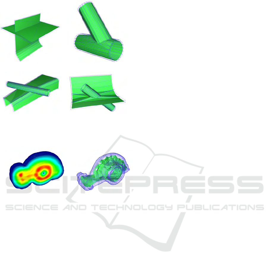
tion and simulation. Figure 6 shows the input data sets

(wire frame in blue) and the corresponding midsur-

faces (in green) of the data sets #1 to #4. The results

fully meet the requirements for midsurfaces.

Nevertheless, a minor problem exist: The limited

precision is based on the grid-based approach and its

cell size; but this problem can be solved at the expense

of resources (memory and time).

The example data set #5, which is not a thin solid,

provides interesting insights into how the algorithm

works (see Figure 7). As the input data set contains

holes and is not manifold, the resulting midsurface

data set #1 data set #2

data set #3 data set #4

Figure 5: The main idea behind using a kernel is to spread

the density values. The overlaps of the kernels at the posi-

tion of the midsurface result in signiﬁcantly higher values

compared to their neighborhood.

Table 4: The characteristic attributes of the input surface ge-

ometry (length of the diagonal of the axis-aligned bounding

box, smallest thickness ε, and greatest thickness δ) allow a

quantitative comparison of input surface geometry and re-

sulting midsurface using the average displacement of ver-

tices and triangles during the vertex climax and vertex clus-

tering steps. The overall comparison is quantiﬁed by the

Hausdorff distance.

data

set

#1 #2 #3 #4 #5

∅ AABB 277.875 248.622 347.048 244.532 9.141

ε 1.770 4.460 0.980 1.510 0.350

δ 4.840 5.220 5.650 6.900 [

0.60 ]

one-sided

distance

vg)

1.912 1.767 1.512 1.552 0.250

(± std)

0.793 1.253 1.182 1.615 0.087

Hausdorf

4.257 5.412 5.039 5.400 0.502

contains holes as well. Due to the grid-based round-

ing and the vertex clustering, the effects are intensify-

ing and the size of the holes increases. In areas which

do not meet the thin solid criteria, the density ﬁeld

does not reveal a consistent directional ﬁeld. There-

fore, the vertex movements within the density ﬁeld

result in self-intersections, which cannot always be

cleared by the mean-shift clustering algorithm.

GRAPP 2021 - 16th International Conference on Computer Graphics Theory and Applications

190

data set #1 data set #2

data set #3 data set #4

Figure 6: This overview shows the input CAD models (wire

frame in blue) and the resulting midsurfaces calculated by

the vertex climax algorithm (in green).

density ﬁeld “midsurface”

Figure 7: If the input surface geometry is not a thin solid

(data set #5), then the accumulated densities (left) do not

lead to a directional ﬁeld that points towards the position of

a midsurface. As a consequence the result is undeﬁned.

5 CONCLUSION

A midsurface consists of surface elements (2D) in or-

der to represent three-dimensional, thin solids whose

local thickness is small compared to its other dimen-

sions. This important representations allow a signif-

icant acceleration of almost all physical simulations.

Unfortunately, midsurfaces are not unique and depend

on their simulation contexts. Although the creation is

a time-consuming, manual step that requires knowl-

edge and experience, it is still the “gold-standard” to

speed up a simulation, if FEM can be replaced by

thin-shell simulations.

5.1 Contribution

The presented approach to extract a midsurface is ap-

plicable to thin-walled parts with a 4-step pipeline

consisting of rasterization of the input geometry to

obtain a grid-based representation, the generation of a

density ﬁeld using a kernel, moving opposing vertices

by a density ﬁeld to iteratively create a thin represen-

tation, and ﬁnally a clustering and cleaning step. The

ﬁrst results of this algorithm deliver satisfying results.

5.2 Beneﬁt

The presented approach generates a midsurface with-

out any manual interaction. Only two geometric val-

ues (the smallest and the greatest thickness) have to

be measured in advance. Once started, no user fur-

ther interaction is needed. As a consequence, the new

approach is suitable for fast feedback loops and rapid

prototyping.

5.3 Open Questions & Future Work

The vertex climax algorithm has only one minor is-

sue: the limited precision. The limited precision will

be addressed by combining the vertex climax algo-

rithm with an automatic mesh generation algorithm.

Having knowledge on the ﬁnite element simulation

performed on a midsurface allows to limit the dis-

cretization artifacts. A locally optimized cell size may

prevent additional discretization errors (on top of the

mesh generation).

In the future, developments will concentrate on

the introduction of local parameters removing the

global constants describing the smallest thickness ε,

and greatest thickness δ. The goal is to determine

these values locally and automatically. In the next

step, the inﬂuence of these parameters will be exam-

ined in more detail.

ACKNOWLEDGEMENTS

The authors would like to thank Ulrich Krispel and

Andreas Riffnaller-Schiefer for fruitful discussions;

Volker Settgast for providing the input data sets and

for his expertise in modeling and construction; Peer

Bertram and Martin Schwarz for their expert knowl-

edge in construction and simulation.

REFERENCES

Aichholzer, O. and Aurenhammer, F. (1996). Straight skele-

tons for general polygonal ﬁgures in the plane. Pro-

ceedings of the International Computing and Combi-

natorics Conference, 2:117–126.

Demuth, M. and Aurenhammer, Franz und Pinz, A. (2010).

Straight skeletons for binary shapes. Computer Vision

Vertex Climax: Converting Geometry into a Non-nanifold Midsurface

191

and Pattern Recognition Workshops (CVPRW), 8:9–

16.

Fujimori, T., Kobayashi, Y., and Suzuki, H. (2006). Sep-

arated medial surface extraction from ct data of ma-

chine parts. Geometric Modeling and Processing,

4077 (LNCS):313–324.

Itoh, T., Yamaguchi, Y., and Koyamada, K. (1996). Volume

thinning for automatic isosurface propagation. Visual-

ization, 7:303–310.

Ju, T., Losasso, F., Schaefer, S., and Waren, J. (2002). Dual

contouring of hermite data. ACM Transactions on

Graphics, 21:339–346.

Kazhdan, M., Bolitho, M., and Hoppe, H. (2006). Poisson

surface reconstruction. Symposium on Geometry Pro-

cessing, 4:61–70.

Kong, T. and Rosenfeld, A. (1989). Digital topology: Intro-

duction and survey. Computer Vision, Graphics, and

Image Processing, 48(3):357–393.

Kulkarni, Y. H. (2016). Development of algorithms for gen-

erating connected midsurfaces using feature informa-

tion in thin walled parts. PhD Thesis at Savitribai

Phule Pune University.

Kulkarni, Y. H. and Kale, M. (2014). Formulating mid-

surface using shape transformations of form features.

Proceedings of All India Manufacturing Technology,

Design and Research, 5:981–985.

Kulkarni, Y. H., Sahasrabudhe, A., and Kale, M. (2017a).

Dimension-reduction technique for polygons. Inter-

national Journal of Computer-Aided Engineering and

Technology, 9:1–17.

Kulkarni, Y. H., Sahasrabudhe, A., and Kale, M. (2017b).

Leveraging feature generalization and decomposition

to compute a wellconnected midsurface. Engineering

with Computers, 33:159–170.

Kwok, P. C. K. and Ranjan, V. (1991). A survey of 3-d

thinning algorithms. Vision Interface, 6:13–20.

Lee, T.-C. and Kashyap, R. L. (1994). Building skele-

ton models via 3-d medial surface/axis thinning al-

gorithms. Graphical Models and Image Processing

(CVGIP), 56:462–478.

Lockett, H. and Guenov, M. (2008). Similarity measures

for mid-surface quality evaluation. Computer-Aided

Design, 40:368–380.

Lorensen, W. E. and Cline, H. E. (1987). Marching cubes:

A high resolution 3d surface construction algorithm.

ACM SIGGRAPH Computer Graphics, 21:163–169.

Ma, C.-M. and Wan, S.-Y. (2001). A medial-surface ori-

ented 3-d two-subﬁeld thinning algorithm. Pattern

Recognition Letters, 22:1439–1446.

Michikawa, T. and Suzuki, H. (2010). Non-manifold medial

surface reconstruction from volumetric data. Geomet-

ric Modeling and Processing, 6130 (LNCS):124–136.

emeth, G., Kardos, P., and Pal

agyi, K. (2010). Topol-

ogy preserving 3d thinning algorithms using four and

eight subﬁelds. Image Analysis and Recognition,

6111:316–325.

Nguyen, Q. T. and Gomes, A. J. P. (2016). Healed marching

cubes algorithm for non-manifold implicit surfaces.

Encontro Portugues de Computacao Graﬁca e Inter-

acao (EPCGI), 23:2:1–8.

Nolan, D. C., Tierney, C. M., Armstrong, C. G., Robinson,

T. T., and Makem, J. E. (2014). Automatic dimen-

sional reduction and meshing of stiffened thin-wall

structures. Engineering with Computers, 30:689–701.

Ogayar-Anguita, C.-J., Rueda-Ruiz, A.-J., Segura-Sanchez,

R.-J., Diaz-Medina, M., and Garcia-Fernandez, A. L.

(2020). A gpu-based framework for generating im-

plicit datasets of voxelized polygonal models for the

training of 3d convolutional neural networks. IEEE

Access, 8:12675–12687.

Pal

agyi, K. and N

emeth, G. (2009). Fully parallel 3d

thinning algorithms based on sufﬁcient conditions for

topology preservation. Discrete Geometry for Com-

puter Imagery (DGCI), 5810 (LNCS):481–492.

Prohaska, S. and Hege, H.-C. (2002). Fast visualization of

plane-like structures in voxel data. IEEE Visualiza-

tion, 13:29–36.

Rezayat, M. (1996). Midsurface abstraction from 3d solid

models: general theory and applications. Computer-

Aided Design, 28:905–915.

Schinko, C., Riffnaller-Schiefer, A., Krispel, U., Eggeling,

E., and Ullrich, T. (2017). State-of-the-art overview

on 3d model representations and transformations in

the context of computer-aided design. International

Journal on Advances in Software, 3 & 4:446–458.

Schinko, C. and Ullrich, T. (2020). A new grid-based mid-

surface generation algorithm. Hyperseeing – the Pub-

lication of the International Society of the Arts, Math-

ematics, and Architecture, 19:81–84.

Schinko, C., Ullrich, T., Schiffer, T., and Fellner, D. W.

(2011). Variance Analysis and Comparison in

Computer-Aided Design. Proceedings of the Inter-

national Workshop on 3D Virtual Reconstruction and

Visualization of Complex Architectures, XXXVIII-

5/W16:3B21–25.

Shawn, M. and Watson, J.-P. (2011). Non-manifold

surface reconstruction from high-dimensional point

cloud data. Computational Geometry, 44:427–441.

Sun, L., Tierney, C. M., Armstrong, C. G., and Robin-

son, T. T. (2016). Automatic decomposition of com-

plex thin walled cad models for hexahedral dominant

meshing. Procedia Engineering, 163:225–237.

Toriwaki, J. and Yonekura, T. (2002). Euler number and

connectivity indexes of a three dimensional digital

picture. Forma, 17:183–209.

Ullrich, T., Settgast, V., and Fellner, D. W. (2008). Ab-

stand: Distance Visualization for Geometric Analy-

sis. Project Paper Proceedings of the Conference on

Virtual Systems and MultiMedia Dedicated to Digital

Heritage (VSMM), 14:334–340.

Woo, Y.-H. and Choo, C.-U. (2009). Automatic genera-

tion of mid-surfaces of solid models by maximal vol-

ume decomposition. Transactions of the Society of

CAD/CAM Engineers, 14:297–305.

Yamzaki, S., Kae, K., and Ikeuchi, K. (2002). Non-

manifold implicit surfaces based on discontinuous im-

plicitization and polygonization. Geometric Modeling

and Processing, 12:138–146.

GRAPP 2021 - 16th International Conference on Computer Graphics Theory and Applications

192