
An Embedded Polygon Strategy for Quality Improvement of 2D
Quadrilateral Meshes with Boundaries
Muhammad Naeem Akram, Lei Si and Guoning Chen
a
University of Houston, Houston, U.S.A.
Keywords:
Quadrilateral Meshes, Quality Improvement, Embedded Polygon.
Abstract:
Quadrilateral (or quad) meshes generated by various remeshing and simplification methods for input models
with complex structure and boundary configurations often possess elements with minimal quality, which calls
for an optimization approach to improve their individual elements’ quality while preserving the boundary
features. Many existing methods either fix boundary vertices during optimization or assume a simple boundary
configuration. In this paper, we introduce a new quality improvement framework for 2D quad meshes with
open boundaries. Our framework aims to optimize the configuration of an embedded polygon constructed
based on the one-ring neighbors of each interior vertex. A feature-preserved boundary optimization is also
introduced based on the angle configuration of the individual boundary vertices to further improve the quality
of the boundary elements. Our framework has been applied to a number of 2D quad meshes with various
boundary configurations and compared with other representative methods to demonstrate its advantages.
1 INTRODUCTION
Quadrilateral (or quad) meshes are preferred by many
mechanical engineering applications due to their de-
sired properties for numerical simulations (Gao et al.,
2017). Numerous efforts have been made to ad-
dress the generation of high-quality quad meshes
(Bommes et al., 2009; Bommes et al., 2013; Campen,
2017; Fang et al., 2018; Viertel and Osting, 2019;
Docampo-Sanchez and Haimes, 2019). Nonethe-
less, robustly generating high-quality quad meshes
for input with arbitrary geometry and topology re-
mains a challenge. Most methods produce initial
quad meshes with sub-optimal quality which require
a post-processing to improve the element quality by
re-positioning the vertices. This post-processing is
called mesh quality improvement. If done properly,
mesh quality improvement can significantly improve
the quality of a mesh (see Figure 5).
Existing quad mesh quality improvement tech-
niques either apply a local tangential space smoothing
(Sorkine, 2005; Daniels et al., 2009; Xu et al., 2018)
after mesh generation or perform re-parameterization,
re-sampling, or edge flipping (Ben-Chen et al., 2008;
Tarini et al., 2011; Pietroni et al., 2009; Prasad,
2018; Gao et al., 2015) during mesh processing. The
smoothing approach preserves the mesh connectivity
a
https://orcid.org/0000-0003-0581-6415
which is required for structured mesh improvement.
However, this constraint may limit its capability of
improving meshes with challenging connectivity con-
figurations. In contrast, the re-parameterization, re-
sampling, or edge-flipping methods optimize the lo-
cal mesh connectivity to achieve better element qual-
ity, while sacrificing the preservation of the structure
of the mesh (i.e., introducing additional irregular ver-
tices). In this work, we focus on the former approach.
Most times, the quality of a quad mesh can be
measured by the scaled Jacobian measures (P
´
ebay
et al., 2007). By definition, the scaled Jacobian mea-
sure of each quad is determined by it’s four interior
angles. A perfect scaled Jacobian (i.e., 1) can be
achieved if all four interior angles are 90
◦
. If one
angle is larger than 180
◦
, the scaled Jacobian be-
comes negative, and the element with negative Jaco-
bian is referred to as an inverted element. An effec-
tive quality improvement technique should remove in-
verted elements in the mesh as much as possible. For
simple quad meshes with non complex structure and
boundaries, smoothing methods like Laplacian mesh
smoothing work well and generate high-quality ele-
ments, but for quad meshes with complex boundaries
(e.g., with many small and sharp features), further
optimization and element refinement is vital in tack-
ling the inverted elements, preserving features, and
smoothing the mesh.
This paper introduces a new quality improvement
Akram, M., Si, L. and Chen, G.
An Embedded Polygon Strategy for Quality Improvement of 2D Quadrilateral Meshes with Boundaries.
DOI: 10.5220/0010209101770184
In Proceedings of the 16th International Joint Conference on Computer Vision, Imaging and Computer Graphics Theory and Applications (VISIGRAPP 2021) - Volume 1: GRAPP, pages
177-184
ISBN: 978-989-758-488-6
Copyright
c
2021 by SCITEPRESS – Science and Technology Publications, Lda. All rights reserved
177

technique, aiming to improve the Jacobian measures
of the mesh. Our method is inspired by Xu and New-
man’s approach (Xu and Newman, 2005) that opti-
mizes the position of a vertex of each quad to be
closer to the bi-sector line of its opposite corner. Dif-
ferent from their method, we optimize the configu-
ration of an embedded polygon surrounding an in-
terior vertex based on its direct one-ring neighbors
(see Figure 1). Furthermore, a boundary optimiza-
tion strategy is introduced to optimize the positions of
boundary vertices based on their angle configuration,
while still preserving boundary features. This enables
further improvement of the quality of the quad ele-
ments at the boundary. We have applied our method
to a number of quad meshes produced by some quad
mesh generation and simplification processes. We
compared the quality of the optimized meshes ob-
tained using our method with those obtained with
Xu and Newman’s method (Xu and Newman, 2005),
Laplacian smoothing (Sorkine, 2005), and Mesquite
(Brewer et al., 2003). The comparison shows that
the optimized meshes with our method usually have
higher minimum and average scaled Jacobians than
those produced by other methods.
2 RELATED WORK
Two different groups of methods have been proposed
for mesh quality improvement, i.e., smoothing and
optimization with fixed mesh connectivity (Vartziotis
and Himpel, 2014; Xu et al., 2018) and local connec-
tivity modification (Prasad, 2018; Tarini et al., 2010;
Gao et al., 2017). The present work belongs to the
former group; thus, we review some representative
methods in this group.
Among all smoothing techniques, Laplacian
smoothing is the most popular technique that aims
to move the individual interior vertices of a mesh to-
ward the average of their direct neighbors. A recent
work shows that Laplacian smoothing is essentially
optimizing the mean ratio quality measure (Vartziotis
and Himpel, 2014). Both explicit (iterative) method
and implicit (direct solving) method (Ji et al., 2005)
of Laplacian smoothing have been proposed. Inter-
ested readers should refer to (Sorkine, 2005; Vartzio-
tis and Himpel, 2014) for a thorough review of Lapla-
cian smoothing and its many variations. Despite its
simplicity and popularity, Laplacian smoothing of-
ten fails for meshes that have undesired connectiv-
ity (especially near the concave area of the bound-
ary) (Canann et al., 1998). Later, optimization-based,
physics-based, or local (Kim et al., 2015) approaches
were introduced to address the limitations of Lapla-
cian smoothing with various levels of success.
Many quad mesh quality improvement methods
are adapted from the techniques for triangle meshes
(Canann et al., 1998), including Laplacian smooth-
ing and its variations. Zhang et al. (Zhang et al.,
2005) proposed a surface mesh smoothing technique
by moving vertices along normal direction based on
a surface diffusion flow. Xu and Newman (Xu and
Newman, 2005) introduced an angle-based optimiza-
tion to optimize the position of each vertex of a quad
to be closer to the bi-sector line of its opposite cor-
ner and neighboring quads. An angle-based smooth-
ing strategy was introduced by Zhou and Shimada
(Zhou and Shimada, 2000) for 2D triangle meshes,
which was later extended by Xu et al. (Xu et al.,
2018) for the hexahedral mesh quality improvement.
Most recently, machine learning technique has been
applied to help address the untangling and smoothing
of meshes (Kim et al., 2020). Our smoothing strat-
egy is most similar to Xu and Newman’s approach
(Xu and Newman, 2005) but with an important dif-
ference, that is, we consider the bisectors of an em-
bedded polygon of each interior vertex (see Figure
1), which reduces the number of angles for consider-
ation by half. In addition, we include weighting strat-
egy and boundary optimization to further improve the
mesh quality.
3 OUR METHOD
We propose a smoothing method that makes use of
circumjacent angles of a vertex to achieve regular-
ization of an embedded polygon formed by one-ring
neighbors. This approach is inspired by a former for-
mulation of an energy function defined by a torsion
springs system. Essentially, the energy based on a
system of torsion spring for a vertex in a mesh can
be defined as (Zhou and Shimada, 2000):
E =
2(n−1)
∑
i=0
1
2
Kθ
2
i
(1)
where, n is the number of polygons incident to the
vertex, θ
i
is the angle between a side of the polygon
and the edge connecting the vertex to the polygon,
and K is a constant. It is not too difficult to see E is
minimum when all θ
i
are identical.
Consider a vertex with n neighbors directly con-
nected to it as shown in Figure 1(a). In this example,
vertex v has four neighbors: v
1
, v
2
, v
3
and v
4
. A poly-
gon can be constructed by connecting the neighbor-
ing vertices of v successively. We call such a poly-
gon an embedded polygon of v as shown with dashed
edges in the example of Figure 1 (a). The shape of
GRAPP 2021 - 16th International Conference on Computer Graphics Theory and Applications
178
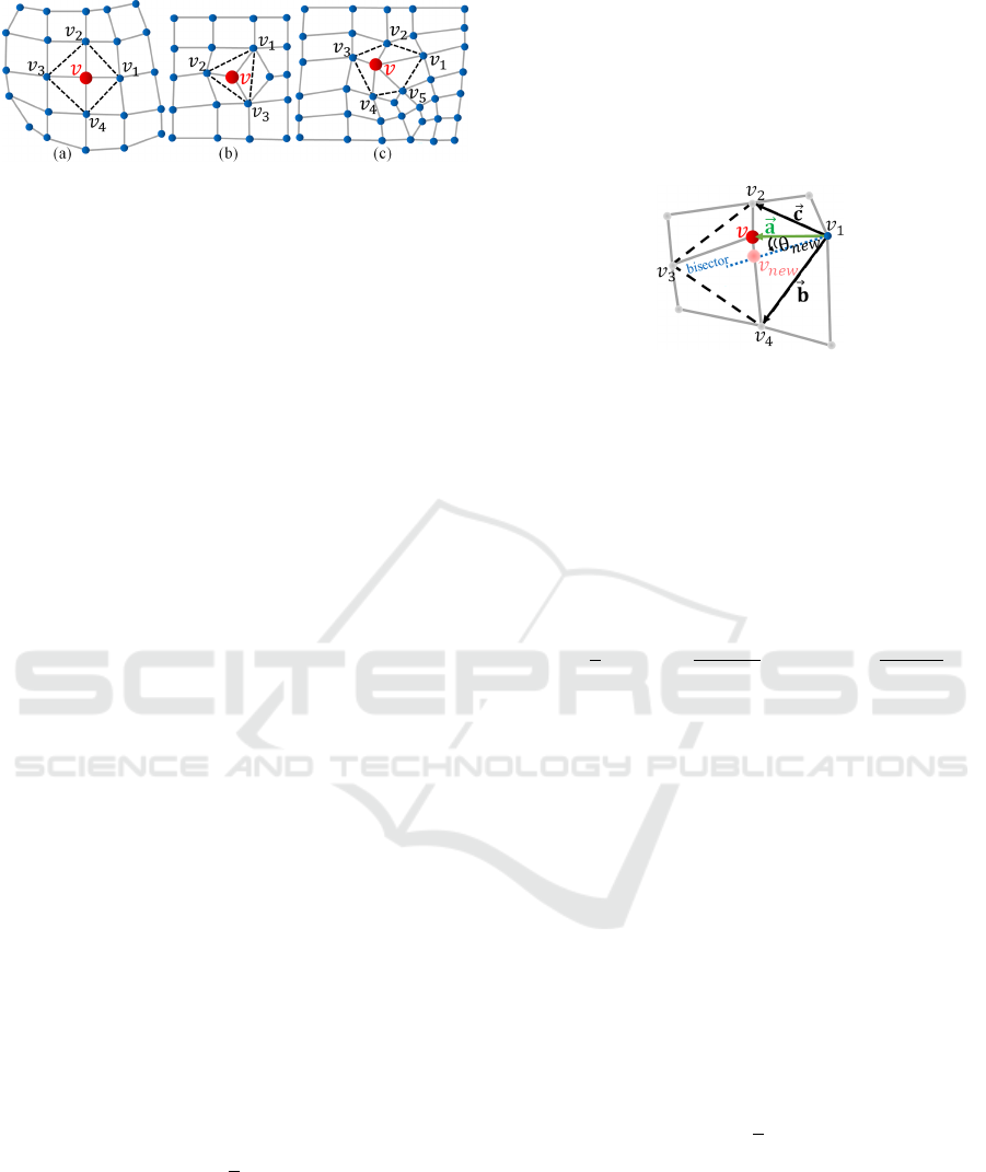
Figure 1: Examples embedded polygons for a valence-4
regular vertex (a), a valence-3 interior vertex (b), and a
valence-5 vertex (c), respectively.
the embedded polygon depends on the number of the
one-ring neighbors adjacent to source vertex (or the
valence of the vertex) (Figure 1(a-c)). The circumja-
cent angles to a vertex are inherently the interior an-
gles of the embedded polygon. A regular embedded
polygon implies that all the interior angles are equal
in magnitude and the source vertex is the centroid of
the embedded polygon being equidistant from all the
adjacent neighbors. In this ideal configuration, the an-
gle bisectors of all the interior angles meet at a single
point. For irregular polygons, however, the interior
angles differ in magnitude and the angle bisectors of
all the interior angles are not equivalent. Thus, the
goal of optimizing the embedded polygon is to make
it as regular as possible, so that the intersections of the
individual bisectors converge to a point, which corre-
sponds to the ideal position of the center vertex.
3.1 Embedded Polygon Optimization
Given a source vertex and its embedded polygon as
illustrated in Figure 2, the position of the vertex can
be updated based on angle bisectors of the interior an-
gles. In an ideal regular polygon, the centroid bisects
all the interior angles of the polygon and the following
relation holds true:
n
∑
i=1
(x
i
− X) = 0 (2)
where, n is the number of one-ring neighbors of a ver-
tex v or sides of the embedded polygon of v, x
i
is the
i
th
angle bisector, and X is the centroid of the em-
bedded polygon. For irregular polygons, solving the
above equation yields:
X =
1
n
n
∑
i=1
x
i
(3)
Therefore, the optimal position of a source vertex v in
its embedded irregular polygon can be achieved in the
following two steps:
1. By updating the interior angles of the embedded
polygon to be identical thus minimizing the en-
ergy function given by Eq.(1).
2. By updating the position of the source vertex to
its optimal value as evidenced by Eq. (3).
In (Xu and Newman, 2005), angles formed by
all the edges between successive neighboring vertices
(adjacent and non-adjacent) are considered while up-
dating the position of the source vertex.
Figure 2: Vertex rotation to bisect interior angle of the em-
bedded polygon.
In contrast, our approach considers the interior an-
gles of the embedded polygon. Therefore, the number
of angles under consideration is reduced in half. From
Figure 2, the interior angles can be bisected by ro-
tating the vectors formed by an edge between source
vertex and the corners of the embedded polygon. For
an interior angle θ, the extent of rotation for the vector
a to bisect the interior angle can be found as:
θ
new
=
1
2
cos
−1
a · b
kakkbk
− cos
−1
a · c
kakkck
(4)
a
new
= b + Ra (5)
where, R =
cosθ
new
−sinθ
new
sinθ
new
cosθ
new
3.2 Interior Vertex Optimization
The rotation of the vertex v to bisect the n interior
angles of the embedded polygon produces a set of n
new coordinates. Consider a set A = {a
1
, a
2
, a
3
, a
4
} of
new coordinates for vertex v generated by its rotation
set B = {θ
1
, θ
2
, θ
3
, θ
4
} to bisect the interior angles of
the embedded polygon. Each of the new coordinates
is a candidate for moving the source vertex towards
the optimal position. The final position of the source
vertex can be calculated by:
v
new
=
1
n
n
∑
i=1
a
i
(6)
This process is analogous to finding an optimal posi-
tion of the source vertex through Laplacian smooth-
ing. However, assigning equal weights to all of the
candidate coordinates can have undesirable effects
during smoothing and the process can sometimes get
stuck between local minimums. To avoid such situ-
ations, weights can be assigned to each item of the
candidate coordinates set A such that the movement
An Embedded Polygon Strategy for Quality Improvement of 2D Quadrilateral Meshes with Boundaries
179
of the source vertex is closest to the optimal position.
For a candidate a in the coordinate set A generated by
its corresponding θ in B, the weight can be assigned
according to the following criteria:
w = 1 −
|θ|
∑
n
i=1
|θ
i
|
(7)
where,
∑
n
i=1
|θ
i
| represents the sum of all rotation an-
gles for vertex v in B. The weights are assigned to
each candidate such that rotation of vertex v for the
worst interior angles bisection of the embedded poly-
gon of v is favored. In this way, the regularity of the
embedded polygon as well as approximation of the
optimal position for vertex v is achieved at a faster
speed since in later iterations of the smoothing pro-
cess, the already bisected angle will have a smaller
weight. The new coordinates v
new
for the source ver-
tex v can be calculated using weights as:
v
new
= λ(
n
∑
i=1
w
i
a
i
− v) (8)
λ is a parameter to control the speed of optimization.
For Laplacian smoothing different λ may affect the
quality of the output. However, in our experiment,
when varying λ between 0.1 and 1, no obvious im-
pact is observed, but larger λ usually results in faster
optimization process. Thus, we set λ = 1. The above
method is similar to Laplacian smoothing (Sorkine,
2005) where the weights are used to determine the
optimal position of a vertex. Hence, the regularity of
the embedded polygon is achieved by making its in-
terior angles close to the ideal angles through the first
part of our approach (Section 3.1) while the optimal
position of the source vertex v in its embedded poly-
gon is achieved through the second part (Section 3.2)
of our approach.
We incorporate collective energy minimization
for the termination decision. The collective energy
E
total
=
∑
n
i
E
i
, where E
i
is given by Eq.(1), can be
computed by calculating and aggregating the ener-
gies of individual embedded polygons associated with
each vertex being optimized. As the optimization ad-
vances, collective mesh energy is calculated before
and after each optimization step and the optimization
is terminated if |E
new
− E
old
| < τ, where τ is a thresh-
old used to determine termination decision.
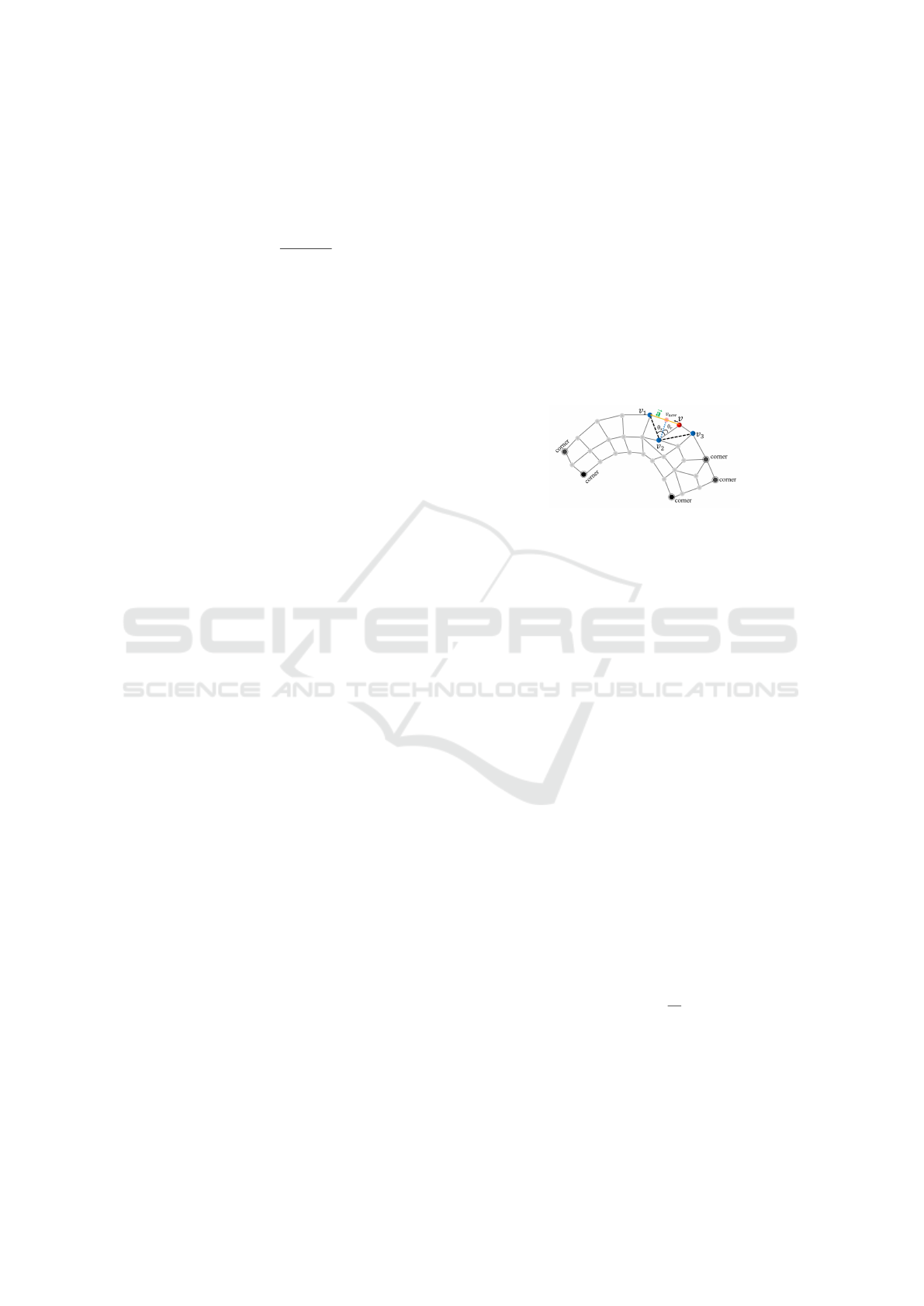
3.3 Boundary Optimization
Feature preservation is usually required during mesh
optimization where certain areas of the mesh are
deemed important in terms of sharp features and cor-
ners and such areas must be preserved during the
mesh optimization to keep the output mesh as close
to the input mesh as possible. In our proposed ap-
proach, we extract the boundary of the input mesh and
regard it as the reference for boundary optimization
and feature preservation. The corners in the bound-
ary are set as immobile (i.e., fixed during boundary
optimization). A corner is a boundary vertex whose
valence is not regular (i.e., the number of quads adja-
cent to this vertex is not 2). To preserve the portion of
the boundary with large curvature and sharp features,
we also mark boundary vertices whose two boundary
edges form an angle θ
b
such that |θ
b
−180
◦
| > c (e.g.,
c = 45
◦
in our experiments). Most of the times, the
sharp features are also singularities as in the case of
Figure 3.
Figure 3: An example illustrating boundary optimization.
A boundary vertex with regular valence (or not
marked as a corner) has a half embedded polygon
with only one full interior angle as shown in Figure
3.
Since only one interior angle is optimized, the sec-
ond part of our method is omitted for boundary opti-
mization. The boundary vertices can be optimized in
two ways:
• Approach 1: Similar to the interior vertices,
boundary vertices can be rotated to bisect the inte-
rior angle of the embedded polygon. The bound-
ary vertex in this case deviates from the boundary
and remapping is required to snap the drifted ver-
tex back to the original boundary. However, some
of the input examples might have complex bound-
ary configuration as shown in Figure 4 (middle)
where the two regions of boundary are very close
to each other and can lead to boundary vertex be-
ing snapped to wrong position.
• Approach 2: The boundary vertices can be re-
stricted to move along the boundary only. From
Figure 3, the new position of vertex v to bisect
the interior angle of the embedded polygon can
be calculated as follows:
v
new
= v + (
θ
r
θ
s
kak) ˆa (9)
Although Approach 2 is more robust than Ap-
proach 1 in handling complicated boundary configu-
rations, as evidenced by Figure 4, in our experiments,
we have observed that the first approach sometimes
produces meshes with better quality for meshes with
GRAPP 2021 - 16th International Conference on Computer Graphics Theory and Applications
180
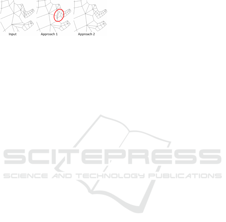
Figure 4: A boundary vertex is incorrectly mapped to a dif-
ferent part of the boundary after the boundary optimization
using the first approach (middle). In contrast, the second
approach preserves the boundary better (right).
simpler boundary configuration (e.g., no or little sharp
features/corners). Therefore, the user can choose ei-
ther of these two approaches to achieve a trade off
between better quality and better boundary preserva-
tion. For both approaches, the boundary optimization
is performed iteratively. We use a similar strategy
for termination of boundary optimization as described
in Section 3.2 with the same threshold τ. Our com-
plete optimization framework incorporates the above
boundary optimization and the interior vertex opti-
mization.
4 RESULTS
We have applied the proposed quality improvement
framework to a number of 2D quad meshes with vary-
ing boundary configurations and mesh connectivity.
Table 1 provides the statistics of the meshes, their
quality before and after optimization, and the run
times. Figure 5 visualizes some representative meshes
before and after optimization with our method. We
use a saturation color coding to show the individual
element quality measured by their scaled Jacobian.
Red indicates low quality elements (i.e., small scaled
Jacobian values) and white indicates elements with
high scaled Jacobian values. From these results, we
can see that the proposed optimization framework sig-
nificantly improves the quality of all these meshes in
terms of their minimum and average scaled Jacobian.
The maximum scaled Jacobian of some meshes does
drop slightly, as it gives more room for more elements
to improve. In practice, the quality of the simulations
(or other scientific computation) run on those meshes
depends on the minimum and average scaled Jacobian
measures as shown by Gao et al. (Gao et al., 2017).
Comparison with Xu and Newman’s Approach.
Figure 6 shows the comparison of our method with
Xu and Newman’s approach. Since their approach as-
sumes fixed boundary vertices during optimization, to
ensure a fair comparison we disable our boundary op-
timization for this comparison. Table 2 provides the
quality statistics of the meshes produced with the two
approaches. Our method without boundary optimiza-
tion generates meshes with better minimum scaled
Jacobian for almost all meshes. More importantly,
our method without boundary optimization produces
meshes with better average scaled Jacobian than Xu
and Newman’s method for all meshes.
Comparison with Laplacian Smoothing and
Mesquite. Here, we compare with two different
variants of Laplacian smoothing, i.e., the Laplacian
with cotangent weights (which we will simply refer
to as Laplacian), and a Laplacian smoothing imple-
mented in a popular mesh quality improvement tool,
Mesquite. Similar to the previous comparison, since
both Laplacian smoothing methods assume fixed
boundaries (otherwise, the mesh will shrink), we
compare our method without boundary optimization
with these two Laplacian smoothing. Figure 7 shows
the meshes produced with the two Laplacian smooth-
ing and our method without boundary optimization.
Table 2 provides the quality statistics of the meshes
produced with the two Laplacian smoothing methods,
labeled as Laplacian and Mesquite, respectively.
From this comparison, we see our method without
boundary optimization outperforms the classic
Laplacian (with cotangent weight) in almost all
meshes except for the minimum scaled Jacobian for
the 1 hole mesh. This matches previous results that
Laplacian smoothing can work well for meshes with
simple boundary configurations. When compared
with the Mesquite results, our method without
boundary optimization produces meshes with better
average scaled Jacobian in almost all cases except
for the 1 hole and 3 hole 1 square. In terms of the
minimum scaled Jacobian, Mesquite produces better
minimum scaled Jacobian measure for five meshes,
i.e., 1 hole, 3 hole, 10 holes, 3 hole 1 square, and
mazewheel. It is worth noting that for patch 7, none
of the existing methods can successfully untangle its
inverted elements (that are highlighted by the black
arrow). In contrast, our method without boundary
optimization can already produce an inversion free
mesh. Nevertheless, by incorporating the boundary
optimization, we can produce the best quality meshes
for all meshes.
Impact of the Threshold Value τ. As described
earlier, a threshold value τ is used to determine when
our optimization should be terminated. In our exper-
iments, we have used different threshold values rang-
ing from 1e
−1
to 1e
−5
. For larger values of τ, the op-
timization algorithm terminates quicker as compared
to smaller values of τ but the extent of optimization
An Embedded Polygon Strategy for Quality Improvement of 2D Quadrilateral Meshes with Boundaries
181
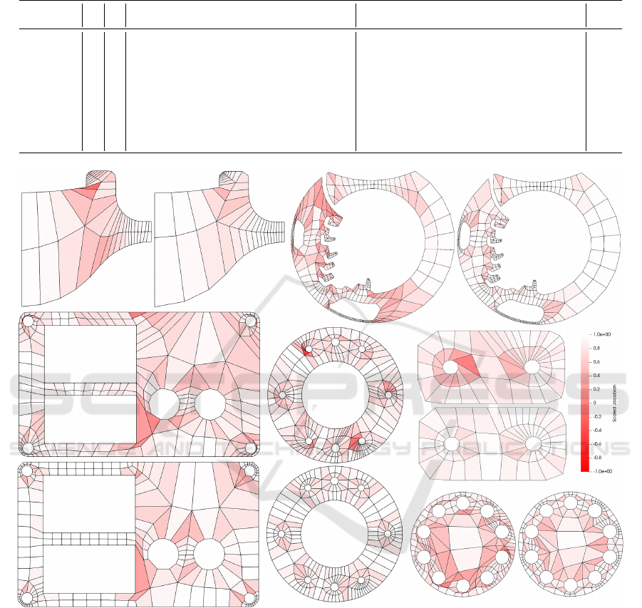
Table 1: Statistics for Scaled Jacobian measure of various meshes before smoothing and after smoothing using our
approach. The best quality measures are highlighted in bold. All results are obtained with the second boundary opti-
mization approach.
Input Output
Model #V #F Min. Scaled Jacobian Avg. Scaled Jacobian Max. Scaled Jacobian Min. Scaled Jacobian Avg. Scaled Jacobian Max. Scaled Jacobian Time (s)
1 hole 69 46 0.558289 0.896226 0.997788 0.742937 0.987127 0.991549 0.29
2 holes 90 61 0.0146683 0.77561 0.981719 0.701665 0.926261 0.993901 0.526
2 holes 2 squares 140 97 -0.556381 0.735316 0.993744 0.197108 0.84893 0.997823 0.112
3 holes 1 square 144 96 0.553854 0.832912 0.997128 0.724021 0.92366 0.998528 0.111
6 holes 2 squares 352 242 -0.164996 0.750487 0.996743 0.296134 0.880297 0.99996 0.547
8 holes 335 229 -0.513426 0.770411 0.999775 0.5811 0.892645 0.999414 0.304
10 holes 288 199 -0.0984454 0.680388 0.995199 0.411444 0.841136 0.995901 0.407
patch 5 87 55 -0.156262 0.756085 0.998083 0.360867 0.838986 0.999841 0.034
patch 7 126 90 -0.528536 0.717805 0.998884 0.312207 0.79753 0.993506 0.06
mazewheel 3 601 392 -0.327252 0.741232 0.999852 0.0558543 0.888563 0.999978 0.81
Figure 5: The representative results of the proposed method. For all meshes, the left (or top) image shows the input mesh
while the right (or bottom) image is the optimized mesh with our method.
is limited. Table 3 summarizes optimization results
for various meshes optimized using different values
of τ. The best quality measures are highlighted in
bold. As can be seen in Table 3, there is not a uni-
versally good τ value for different meshes. Thus, we
leave this threshold value for the user to decide.
5 CONCLUSION
This paper presents a new quality improvement
method for 2D quad meshes with open boundaries.
Our method is based on the optimization of the con-
figuration of an embedded polygon constructed for
each interior vertex. A feature preserving boundary
optimization is also introduced. We have applied our
framework to a number of 2D quad meshes to eval-
uate its effectiveness. We also compare our method
GRAPP 2021 - 16th International Conference on Computer Graphics Theory and Applications
182
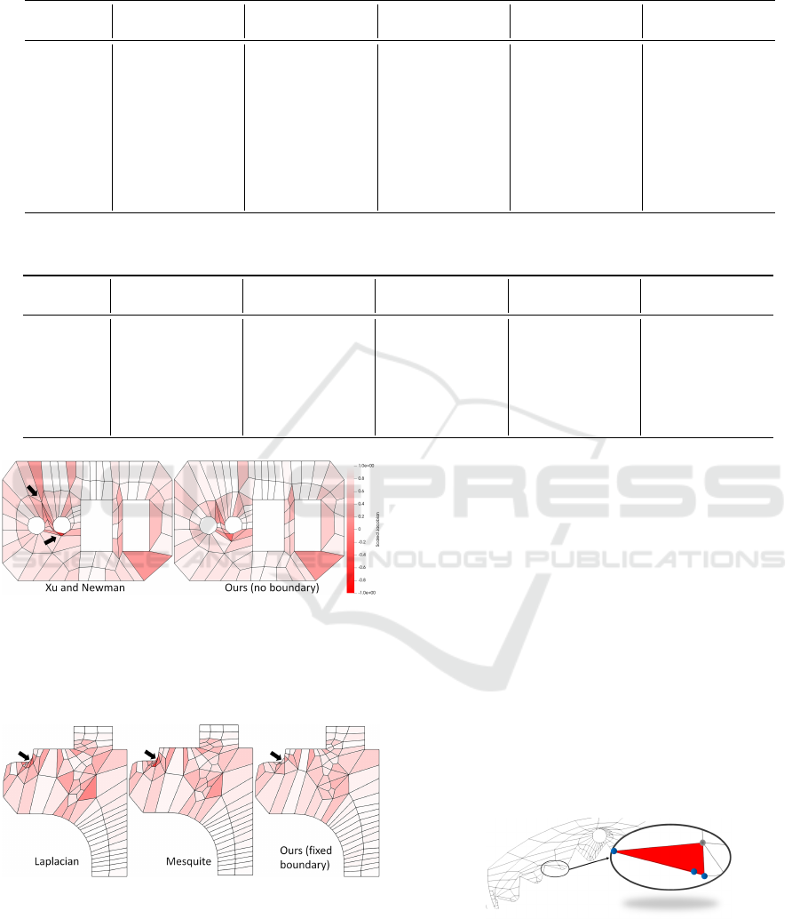
Table 2: Statistics of Scaled Jacobian measures of various meshes optimized with different methods. The best quality
measures of all results are highlighted in bold. The best quality measures of the results produced by methods with fixed
boundaries are highlighted in blue.
Xu and Newman Laplacian Mesquite Ours w/o bound Ours w bound
Model Min. Scaled Avg. Scaled Min. Scaled Avg. Scaled Min. Scaled Avg. Scaled Min. Scaled Avg. Scaled Min. Scaled Avg. Scaled
1 hole 0.558289 0.899476 0.640883 0.899255 0.643728 0.902054 0.614279 0.8973 0.97646 0.987127
2 holes 0.166075 0.79649 -0.0158924 0.773395 0.0205342 0.774537 0.0811026 0.777924 0.742937 0.926261
2 holes 2 squares -0.556381 0.752143 -0.453973 0.735066 -0.487485 0.738351 -0.15848 0.782632 0.197108 0.84893
3 holes 1 square 0.559189 0.842663 0.538608 0.833651 0.57367 0.838737 0.563918 0.83856 0.724021 0.92366
6 holes 2 squares -0.164996 0.761158 -0.36941 0.749143 -0.28024 0.760459 -0.117874 0.785367 0.296134 0.880297
8 holes -0.513426 0.767459 -0.544005 0.765766 -0.47977 0.772616 -0.147611 0.788872 0.5811 0.892645
10 holes -0.0984454 0.783175 -0.246311 0.675738 -0.188317 0.686278 -0.201791 0.708256 0.411444 0.841136
patch 5 -0.0247695 0.776693 -0.176222 0.750139 -0.15496 0.759693 -0.0813105 0.818403 0.360867 0.838986
patch 7 -0.528536 0.724826 -0.147158 0.727404 -0.556283 0.728614 0.276863 0.789242 0.312207 0.79753
mazewheel 3 -0.458242 0.745167 -0.699953 0.735654 -0.653876 0.742469 -0.65144 0.761198 0.0558543 0.888563
Table 3: Effect of different threshold (τ) values on mesh optimization using our method on a number of representative
meshes. The best quality measures are highlighted in bold.
τ = 0.1 τ = 0.01 τ = 0.001 τ = 0.0001 τ = 0.00001
Model Min. Scaled Avg. Scaled Min. Scaled Avg. Scaled Min. Scaled Avg. Scaled Min. Scaled Avg. Scaled Min. Scaled Avg. Scaled
2 holes 2 squares 0.197108 0.847687 0.197108 0.849726 0.197108 0.849073 0.197108 0.84893 0.197108 0.84893
3 holes 1 square 0.720105 0.920828 0.721011 0.923883 0.723246 0.923717 0.724021 0.92366 0.724161 0.923631
6 holes 2 squares 0.318459 0.882613 0.320006 0.880864 0.298935 0.880412 0.296134 0.880297 0.29614 0.880295
8 holes 0.58685 0.891942 0.582073 0.892883 0.580989 0.89271 0.5811 0.892645 0.581242 0.892652
10 holes 0.413944 0.843625 0.411547 0.841411 0.411444 0.841136 0.411444 0.841136 0.449502 0.841136
patch 7 0.251875 0.794919 0.303568 0.797214 0.303568 0.797214 0.312207 0.79753 0.312207 0.79753
mazewheel 3 0.0066067 0.88877 0.0411956 0.88851 0.0518666 0.888541 0.0558543 0.888563 0.0566735 0.888568
Figure 6: Comparison of our method (right) with Xu and
Newman’s approach (left). The arrows indicate places that
the mesh quality in the results of Xu and Newman’s ap-
proach is less desired. The 2 holes with 2 square mesh is
shown. Red color indicate quad elements with low Jaco-
bian measures.
Figure 7: Comparison with conventional Laplacian smooth-
ing with cotangent weights and the Laplacian smoothing
implemented in Mesquite. The patch 7 mesh is shown. Red
color indicate quad elements with low Jacobian measures.
The arrows highlight area with elements that other methods
fail to improve, while our method can.
with a number of the state-of-the-art quad mesh opti-
mization methods. The comparison shows that our
method outperforms the existing methods in most
cases, especially for meshes with many complicated
boundary features.
Limitation and Future Work. Even though our
method is simple and easy to implement and has
shown outperforming many state-of-the-art methods
in most cases, our method cannot guarantee to always
produce inversion-free mesh. As shown in the inset,
our method fails to untangle an inverted element in
the mazewheel mesh. A closer look shows that three
vertices of this inverted element are on the boundary,
and two of them are corners, thus, fixed. These three
vertices form a concave configuration with an inner
angle larger than 180
◦
.
In fact, no smoothing method can fix this unless
this boundary is modified to make the angle smaller
than 180
◦
. Alternatively, a local connectivity modifi-
cation may help mitigate this situation, which is be-
yond the scope of this work.
An Embedded Polygon Strategy for Quality Improvement of 2D Quadrilateral Meshes with Boundaries
183

Our current framework provides two different
ways for boundary optimization. In the future, it will
be more ideal to have an automatic way to decide
the proper boundary optimization based on the input
mesh configuration without user intervention.
ACKNOWLEDGEMENTS
We thank the anonymous reviewers for their valuable
feedback. This research was partially supported by
NSF IIS 1553329.
REFERENCES
Ben-Chen, M., Gotsman, C., and Bunin, G. (2008). Con-
formal flattening by curvature prescription and metric
scaling. In Computer Graphics Forum, volume 27,
pages 449–458. Wiley Online Library.
Bommes, D., L
´
evy, B., Pietroni, N., Puppo, E., Silva, C.,
Tarini, M., and Zorin, D. (2013). Quad-mesh gener-
ation and processing: A survey. In Computer Graph-
ics Forum, volume 32, pages 51–76. Wiley Online Li-
brary.
Bommes, D., Zimmer, H., and Kobbelt, L. (2009). Mixed-
integer quadrangulation. ACM Trans. Graph., 28(3).
Brewer, M. L., Diachin, L. F., Knupp, P. M., Leurent, T.,
and Melander, D. J. (2003). The Mesquite Mesh Qual-
ity Improvement Toolkit. In Shepherd, J., editor, IMR.
Campen, M. (2017). Partitioning surfaces into quadrilat-
eral patches: a survey. In Computer Graphics Forum,
volume 36, pages 567–588. Wiley Online Library.
Canann, S. A., Tristano, J. R., Staten, M. L., et al. (1998).
An approach to combined laplacian and optimization-
based smoothing for triangular, quadrilateral, and
quad-dominant meshes. In IMR, pages 479–494. Cite-
seer.
Daniels, J., Silva, C. T., and Cohen, E. (2009). Localized
quadrilateral coarsening. In Computer Graphics Fo-
rum, volume 28, pages 1437–1444. Wiley Online Li-
brary.
Docampo-Sanchez, J. and Haimes, R. (2019). Towards fully
regular quad mesh generation. In AIAA Scitech 2019
Forum, page 1988.
Fang, X., Bao, H., Tong, Y., Desbrun, M., and
Huang, J. (2018). Quadrangulation through morse-
parameterization hybridization. ACM Transactions on
Graphics (TOG), 37(4):92.
Gao, X., Deng, Z., and Chen, G. (2015). Hexahedral mesh
re-parameterization from aligned base-complex. ACM
Transactions on Graphics (TOG), 34(4):1–10.
Gao, X., Huang, J., Xu, K., Pan, Z., Deng, Z., and Chen,
G. (2017). Evaluating hex-mesh quality metrics via
correlation analysis. In Computer Graphics Forum,
volume 36, pages 105–116. Wiley Online Library.
Ji, Z., Liu, L., and Wang, G. (2005). A global lapla-
cian smoothing approach with feature preservation. In
Ninth International Conference on Computer Aided
Design and Computer Graphics (CAD-CG’05), pages
6–pp. IEEE.
Kim, J., Choi, J., and Kang, W. (2020). A data-driven ap-
proach for simultaneous mesh untangling and smooth-
ing using pointer networks. IEEE Access, 8:70329–
70342.
Kim, J., Shin, M., and Kang, W. (2015). A derivative-
free mesh optimization algorithm for mesh quality im-
provement and untangling. Mathematical Problems in
Engineering, 2015.
P
´
ebay, P. P., Thompson, D. C., Shepherd, J., Knupp, P. M.,
Lisle, C., Magnotta, V., and Grosland, N. M. (2007).
New Applications of the Verdict Library for Standard-
ized Mesh Verification Pre, Post, and End-to-End Pro-
cessing. In Brewer, M. L. and Marcum, D. L., editors,
IMR, pages 535–552. Springer.
Pietroni, N., Tarini, M., and Cignoni, P. (2009). Almost
isometric mesh parameterization through abstract do-
mains. IEEE Transactions on Visualization and Com-
puter Graphics, 16(4):621–635.
Prasad, T. (2018). A comparative study of mesh smooth-
ing methods with flipping in 2D and 3D. PhD thesis,
Rutgers University-Camden Graduate School.
Sorkine, O. (2005). Laplacian Mesh Processing. In
Chrysanthou, Y. and Magnor, M., editors, Eurograph-
ics 2005 - State of the Art Reports. The Eurographics
Association.
Tarini, M., Pietroni, N., Cignoni, P., Panozzo, D., and
Puppo, E. (2010). Practical quad mesh simplification.
In Computer Graphics Forum, volume 29, pages 407–
418. Wiley Online Library.
Tarini, M., Puppo, E., Panozzo, D., Pietroni, N., and
Cignoni, P. (2011). Simple quad domains for field
aligned mesh parametrization. In Proceedings of the
2011 SIGGRAPH Asia Conference, pages 1–12.
Vartziotis, D. and Himpel, B. (2014). Laplacian smoothing
revisited. arXiv preprint arXiv:1406.4333.
Viertel, R. and Osting, B. (2019). An approach to quad
meshing based on harmonic cross-valued maps and
the ginzburg–landau theory. SIAM Journal on Scien-
tific Computing, 41(1):A452–A479.
Xu, H. and Newman, T. S. (2005). 2d fe quad mesh smooth-
ing via angle-based optimization. In International
Conference on Computational Science, pages 9–16.
Springer.
Xu, K., Gao, X., and Chen, G. (2018). Hexahedral
mesh quality improvement via edge-angle optimiza-
tion. Computers & Graphics, 70:17–27.
Zhang, Y., Bajaj, C. L., and Xu, G. (2005). Surface
Smoothing and Quality Improvement of Quadrilat-
eral/Hexahedral Meshes with Geometric Flow. In
Hanks, B. W., editor, IMR, pages 449–468. Springer.
Zhou, T. and Shimada, K. (2000). An angle-based approach
to two-dimensional mesh smoothing. IMR, 2000:373–
384.
GRAPP 2021 - 16th International Conference on Computer Graphics Theory and Applications
184
