Sewer Defect Classification using Synthetic Point Clouds
Joakim Bruslund Haurum
a,§
, Moaaz M. J. Allahham
b,∗
, Mathias S. Lynge
c,†
,
Kasper Schøn Henriksen
d,‡
, Ivan A. Nikolov
e,∗∗
and Thomas B. Moeslund
f,††
Visual Analysis of People (VAP) Laboratory, Aalborg University, Rendsburggade 14, Aalborg, Denmark
{mallah16
∗
, mlynge16
†
, kshe16
‡ §
, iani
∗∗
, tbm
††
Keywords:
3D Deep Learning, Defect Classification, Synthetic Data, Sewers, Point Clouds, Transfer Learning.
Abstract:
Sewer pipes are currently manually inspected by trained inspectors, making the process prone to human errors,
which can be potentially critical. There is therefore a great research and industry interest in automating the
sewer inspection process. Previous research have been focused on working with 2D image data, similar to how
inspections are currently conducted. There is, however, a clear potential for utilizing recent advances within
3D computer vision for this task. In this paper we investigate the feasibility of applying two modern deep
learning methods, DGCNN and PointNet, on a new publicly available sewer point cloud dataset. As point
cloud data from real sewers is scarce, we investigate using synthetic data to bootstrap the training process.
We investigate four data scenarios, and find that training on synthetic data and fine-tune on real data gives the
best results, increasing the metrics by 6-10 percentage points for the best model. Data and code is available at
https://bitbucket.org/aauvap/sewer3dclassification.
1 INTRODUCTION
The sewerage infrastructure is one of the largest, but
also most forgotten, infrastructures in our modern so-
ciety. In the United States there are currently approxi-
mately 2 million km of sewer pipes serving nearly 240
million Americans. By 2036 the sewerage infrastruc-
ture is expected to serve an additional 56 million users
(American Society of Civil Engineers, 2017). The
size of the sewerage infrastructure poses a clear prob-
lem during maintenance, as it is near impossible to
regularly inspect all stretches of sewer pipes. Further-
more, sewer maintenance requires skilled inspectors
who are capable of operating the required equipment
to inspect the buried pipes. These inspections are
conducted using a remote-controlled “tractor”, which
the inspector controls from a vehicle above ground.
This can be both demanding and slow, and potentially
prone to human errors.
To deal with this problem, one possibility is to
use an autonomous or semi-autonomous robotic so-
lution. Such solutions have been successfully de-
a
https://orcid.org/0000-0002-0544-0422
b
https://orcid.org/0000-0002-3212-0731
c
https://orcid.org/0000-0002-8492-1274
d
https://orcid.org/0000-0001-8660-1672
e
https://orcid.org/0000-0002-4952-8848
f
https://orcid.org/0000-0001-7584-5209
veloped and deployed for tunnel walls inspection
(Menendez et al., 2018), transmission and electrical
wires (Qin et al., 2018), underwater ship hulls (Gar-
rido et al., 2018), wind turbine blades (Car et al.,
2020), among others. An important characteristic that
each of these solutions share, is that the robotic sys-
tem needs to have appropriate sensors for both self-
localization and mapping the environment, as well as
capturing enough information from the surfaces such
that a proper inspection of potential damages or ob-
structions can be achieved. To ensure that enough in-
formation is captured, 3D information in the form of
depth images and point clouds, is chosen in addition
to traditional 2D images. To capture such informa-
tion, different sensor can be used - LiDAR laser scan-
ners (Nasrollahi et al., 2019; Ravi et al., 2020), stereo
cameras (Wen et al., 2017), photogrammetry (Nielsen
et al., 2020), time-of-flight and structured light cam-
eras (Pham et al., 2016; Santur et al., 2016).
Sewer inspection data presented in the state-of-
the-art is normally not available as public datasets,
and the ones used are focused around 2D RGB im-
ages (Haurum and Moeslund, 2020). However, cap-
turing large amounts of 3D inspection data from sew-
ers is not a trivial task. Therefore, we look into us-
ing synthetic data for training a sewer inspection al-
gorithm. The creation of such synthetic data has been
detailed in the work of Henriksen et al. (2020), where
Haurum, J., Allahham, M., Lynge, M., Henriksen, K., Nikolov, I. and Moeslund, T.
Sewer Defect Classification using Synthetic Point Clouds.
DOI: 10.5220/0010207908910900
In Proceedings of the 16th International Joint Conference on Computer Vision, Imaging and Computer Graphics Theory and Applications (VISIGRAPP 2021) - Volume 5: VISAPP, pages
891-900
ISBN: 978-989-758-488-6
Copyright
c
 2021 by SCITEPRESS – Science and Technology Publications, Lda. All rights reserved
891

sewer pipes were 3D modeled and used in a cus-
tom simulation environment, together with an approx-
imated PMD Pico Flexx (CamBoard, 2018) time-of-
flight camera, to generate 3D point clouds. We there-
fore look into using synthetic data to bootstrap the
training process of a deep learning based 3D sewer
defect classifier. The main contributions of this paper
are threefold:
1. A publicly available dataset of synthetic and real
point clouds of normal and defective sewer pipes.
2. Demonstrating the feasibility of using 3D point
clouds and geometric deep learning methods for
classifying sewer defects.
3. A comparison of the effect of synthetic and/or real
data when training a defect classifier.
2 RELATED WORK
Automated Sewer Inspections. Vision-based
automation of sewer defects has traditionally been
based on 2D image data from Closed-Circuit Tele-
vision (CCTV) and Sewer Scanner and Evaluation
Technology (SSET) sewer inspections. CCTV and
SSET inspection data have been used for nearly
30 years, with methods ranging from morphology
based discriminators (Sinha and Fieguth, 2006a,b,c;
Su et al., 2011), to using feature descriptors and
machine learning classifiers (Yang and Su, 2008; Wu
et al., 2013; Myrans et al., 2018), and within the
recent years using deep learning for classification,
detection, and segmentation (Hassan et al., 2019; Li
et al., 2019; Kumar et al., 2020; Wang and Cheng,
2020). For an in-depth review of these methods we
refer to the survey by Haurum and Moeslund (2020).
There has, however, been significantly less work on
detecting defects using 3D sensors. 3D sensors are
interesting as some sewer defects, such as displaced
joints and obstacles, may not be immediately visually
apparent, but can be obvious when looking at the
depth information. Traditionally two types of sensors
have been used: Laser scanners and ultrasound. Laser
scanners have been used extensively by Duran et al.
for binary defect detection of cracks, defective joints,
and obstacles, by utilizing depth and the intensity of
the reflected light as input for fully-connected neural
networks (Duran et al., 2003, 2004, 2007). Similarly,
Lepot et al. (2017) designed a novel laser scanner
for detecting displaced joints, cracks, and deposits,
which works in a comparable way as to CCTV in-
spections. Tezerjani et al. (2015) similarly proposed
a novel laser scanner design for defect detection
and extracting pipe geometry. Furthermore, Ahrary
et al. (2006) and Kolesnik and Baratoff (2000) have
used laser scanners for navigation purposes as well
as detecting defects and recovering the geometry of
the pipe. Iyer et al. (2012) utilized ultrasound based
methods for detecting cracks and holes in concrete
pipes. Khan and Patil have proposed detection cracks
in PVC pipes by analyzing the acoustic response
under different conditions using frequency domain
analysis (Khan and Patil, 2018a,b). Alejo et al.
have utilized RGB-D camera for localization and
defect classification, utilizing graph based learning
and convolutional neural networks (CNN) (Alejo
et al., 2017, 2020). Furthermore, as documented
by Haurum and Moeslund (2020) there is a lack of
public dataset and code releases for methods based
on CCTV and SSET inspections, which is also the
case with methods designed for inspections using 3D
sensors.
Geometric Deep Learning. Within recent years the
application of deep learning methods on unstructured
3D data, such as point clouds, have gained interest
within the computer vision community. The earliest
methods utilized specialized voxel-based methods
(Qi et al., 2016) and reutilizing 2D CNNs in a
multiview-based approach (Su et al., 2015) in order
to classify objects, resulting in, respectively, high
memory consumption and slow computation times.
Qi et al. were the first to successfully process the
raw point clouds using the fully-connected neural
network architectures, PointNet (Qi et al., 2017a)
and PointNet++ (Qi et al., 2017b). This work has
been expanded upon within the autonomous vehicle
community for object detection and segmentation
(Lang et al., 2019; Vora et al., 2020), amongst other
point based methods (Zhou and Tuzel, 2018; Wang
et al., 2019). 3D point clouds can also be observed
as a graph problem, which was utilized by Wang
et al. (2019) in the Dynamic Graph CNN (DGCNN)
architecture, where edge information between points
are aggregated to better learn local and global infor-
mation. For a review of the geometric deep learning
field we refer to the work of Bronstein et al. (2017)
and Cao et al. (2020).
Synthetic Data. In the current era of machine learn-
ing based methods, representative training data is es-
sential. However, it may not always be possible to
acquire the necessary training data, as it can be pro-
hibitively expensive. This is especially apparent when
working on tasks where the interesting parts are rare,
such as defect detection. The generation of represen-
tative synthetic data has therefore been increasingly
investigated. Tobin et al. (2017) proposed the Do-
VISAPP 2021 - 16th International Conference on Computer Vision Theory and Applications
892

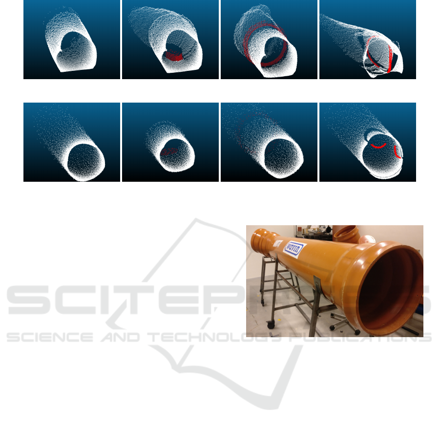
(a) Phys. Normal (b) Phys. Brick (c) Phys. Disp. (d) Phys. Ring
(e) Synth. Normal (f) Synth. Brick (g) Synth. Disp. (h) Synth. Ring
Figure 1: Example point clouds from the real and synthetic pipe setup. Defects are shown in red for easier visualization.
main Randomization (DR) method, which generates
randomized renderings of a scene in order to train a
robot. Prakash et al. (2019) expanded on this method
by accounting for the structure in the scene, called
Structured Domain Randomization (SDR), which was
demonstrated on the KITTY object detection task.
Beery et al. (2020) showed using large amount of syn-
thetic data can help handle the long tailed distribution
that occurs in the animal classification task, showing
the promise of synthetic data. Lastly, Henriksen et al.
(2020) proposed an SDR based synthetic data gen-
erator for PVC sewer pipes, which can generate dis-
placed joints and defective rubber rings in the joints.
3 DATASET
As mentioned in Section 2 there are currently no pub-
licly available datasets within the sewer inspection
field. We therefore construct our own dataset, consist-
ing of normal non-defective pipes and defective pipes
with three different kinds of defects: displaced joints,
defective rubber rings, and obstructions in the form of
bricks. The three defect types are selected as they are
observed frequently in the real world. As 3D sensors
are very rarely used for sewer inspections, the con-
structed dataset consists of synthetic point cloud data,
as well as real data obtained in a lab environment.
3.1 Synthetic Data Generation
We base our synthetic data generation on the SDR-
based approach proposed by Henriksen et al. (2020).
The proposed data generator generates a random
Figure 2: An example pipe configuration, used for collect-
ing the point cloud data from the physical setup.
sewer network consisting of clean PVC pipes, with
no water or sediments, and randomly places defects
along the pipes. A virtual approximation of the PMD
Pico Flexx time-of-flight sensor is moved through the
sewer network, and record synthetic point clouds.
The generated defects are, however, constrained
to only displaced joints and defective rubber rings,
which are concurrent. We update the simulator to al-
low displaced joints and defective rubber rings to oc-
cur independent of each other, and further extend it to
allow for randomly placed bricks in the pipe. Bricks
are chosen, because of their relatively basic shape, not
prone to many variations, compared to other possible
obstructions in sewer pipes. This way the overall de-
fect classification performance of the algorithms can
be evaluated, without the need to create too many dif-
ferent shape cases. The bricks are placed by applying
a random force to the brick, which pushes it into a
random position and orientation in the pipe. We con-
strain the simulator to only allow one kind of defect
per extracted point cloud, in order to be able to deter-
Sewer Defect Classification using Synthetic Point Clouds
893

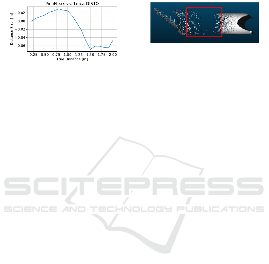
Figure 3: The Pico Flexx distance errors, compared to a
laser range finder at distances between 0.2m and 2m.
mine the effect of each type of defect.
3.2 Physical Data Collection
In order to collect point clouds from a set of real PVC
sewer pipes, a physical setup was created in an indoor
laboratory, see Figure 2. The data was collected using
a PMD Pico Flex sensor. As no sewer data captured
with the Pico Flex sensor is available, we conduct
a simple test, to verify its accuracy presented in its
datasheet (CamBoard, 2018). The sensor is mounted
on a moving platform and directed towards a white
wall with an approximately Lambertian surface. The
sensor is then moved away from the wall at equal
0.1m intervals, starting from 0.2m until 2m. A Leica
DISTO laser range finder, is used to capture ground
truth data at each position, as it has a known accuracy
of 0.03m. The two sensors are calibrated to the same
distance measurement at 0.2m. The difference be-
tween the two are presented on Figure 3. The distance
errors are higher than the ones given in the datasheet
CamBoard (2018) for the camera. This needs to be
taken into account, as these distance errors, might re-
sult in noise or deformations in the selected pipe seg-
ments, especially between 0.8m and 1.5m.
Five different pipe segments, with a diameter of
400 mm were used for data collection: two straight
pipes, and three corner pipes with turning angles of
15, 30, and 45 degrees. The pipe segments were com-
bined in different permutation, with the sensor moved
through the pipes while placed in the center. Defects
were added to the pipes by randomly placing bricks
or rubber rings in the pipes, or displacing the joints of
the pipe segments. As in the synthetic data generator,
only one type of defect is present at a time.
3.3 Comparison between Real and
Synthetic Data
Examples of the real and synthetic data are shown in
Figure 1, with one example per class. One problem
found from the real data captured with the Pico Flexx
Figure 4: Example of point clouds captured with the real
Pico Flexx and the holes, caused by missing data.
sensor, is the presence of “holes” in both the depth
map and the point cloud - areas, where no depth data
is captured. These holes depend on the environmen-
tal lighting, the distance and orientation of the imaged
surface, compared to the camera, as well as the glossi-
ness of the surface. Examples of such holes can be
seen in Figure 4. One way we address this problem
is by subsampling both the synthetic and real point
cloud data, which lowers the density variation of the
point clouds. More information, about the subsam-
pling process can be found in Section 4.1.
3.4 Dataset Split
The acquired synthetic and real data are divided into
training, validation and test splits, as shown in Table
1. We choose to place the majority of the real data
(85%) in the test split, as to reflect the real world
data situation, where inspection data is in the form
of CCTV and SSET videos and annotated 3D data is
limited. Inversely, we utilize the majority of the syn-
thetic data in the training and validation splits. We
make sure there is no data leakage between splits by
generating new synthetic data for each split, and split-
ting the real data based on the pipe segment configu-
rations. We balance the amount of defective and nor-
mal data, such that the problem is more well-behaved,
which is standard within the sewer defect classifica-
tion field (Li et al., 2019; Hassan et al., 2019).
4 METHODS
The proposed method consists of two steps: prepro-
cessing the data and the deep learning models.
4.1 Data Preprocessing
Training a deep learning model on the raw point cloud
data is infeasible due to the large number of points,
leading to high memory consumption. It is therefore
necessary to subsample the point clouds in order to
efficiently process them. Before subsampling point
clouds, it is preferred to reduce the number of out-
liers that may occur. This can prevent subsampling
VISAPP 2021 - 16th International Conference on Computer Vision Theory and Applications
894

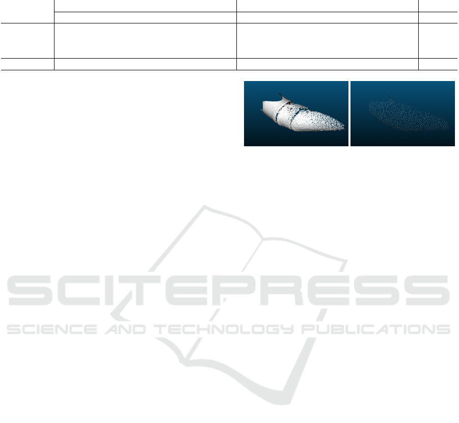
Table 1: Overview of the data in the different data splits. The Displacement (Disp.), Brick, and Rubber Ring columns represent
the amount of point clouds for the three investigated defect types.
Synthetic Real
Split Normal Disp. Brick Rubber Ring Normal Disp. Brick Rubber Ring Total
Training 5,365 1,811 1,822 1,802 140 45 45 44 11,074
Validation 1,385 439 428 448 31 12 12 13 2,768
Test 1,350 450 450 450 244 85 76 80 3,185
Total 8,100 2,700 2,700 2,700 415 142 133 137 17,027
approaches being biased by the outliers and rather fo-
cus on points containing relevant geometric informa-
tion of a given pipe. Points that are stored in the origin
of a point cloud are discarded, as they represent points
that did not return a valid value. Afterwards, Statisti-
cal Outlier Removal (SOR) (Barnett and Lewis, 1984)
is applied to discard aberrative points that heavily dif-
fer from the geometric representation of a pipe.
We subsample the point clouds to 1024 points, the
number of points originally used for the PointNet ap-
proach. Traditionally the subsampling step has been
performed by applying the Farthest Point Sampling
method, which iteratively selects the point in the point
cloud which is farthest away from the previously se-
lected points (Qi et al., 2017a). This is, however,
not the best approach for our data, as some defects
manifest themselves as points in the middle of the
pipe, which would be subsequently removed. There-
fore we apply two different subsampling approaches
sequentially. First we apply a spatial subsampling
step Rousseeuw and Leroy (2005), which enforces a
minimum distance, d, between each point. d is se-
lected such that more than 1024 points remain, though
d may change per point cloud. d is initially set to
0.03, and decremented by 0.004 each time the result-
ing point cloud has less than 1024 points. Afterwards
the point cloud is reduced to 1024 through uniformly
sampling the subsampled point cloud. As a last step
the subsampled point clouds are normalized into a
unit sphere. Examples of a pipe segment before and
after the preprocessing steps can be seen in Figure 5.
4.2 Model Architectures
We investigate the performance of two state-of-the-
art geometric deep learning methods: PointNet (Qi
et al., 2017a) and DGCNN (Wang et al., 2019).
We choose PointNet to get a baseline performance,
whereas DGCNN is chosen to evaluate the effective-
ness of the advances within the field. PointNet is built
upon sequentially applying the same fully-connected
sub-networks on the individual points, in parallel.
This way each point is processed independently of
any other points. In order to aggregate the feature
information of each point, the symmetric max pool-
(a) Before Subsampling (b) After Subsampling
Figure 5: Example of a sewer pipe segment before and after
the subsampling preprocessing steps.
ing function is used. Furthermore, the PointNet archi-
tecture includes a special sub-network called a T-Net,
which predicts an affine transformation matrix used
to align the input into a canonical form. The T-Net
is applied in the beginning on the raw input, as well
as the intermediate features. However, the intermedi-
ate feature alignment matrix is learned in a high di-
mensional space, which makes the optimization pro-
cess more difficult (Qi et al., 2017a). Therefore, Qi
et al. (2017a) regularize the feature alignment matrix,
A, by forcing it to be close to an orthogonal matrix, as
shown in Equation 1.
L
reg
= ||I − AA
T
||
2
F
(1)
The DGCNN network builds upon the PointNet archi-
tecture, by introducing the EdgeConv layer between
each of the shared fully-connected subnetworks. For
each point, x
i
, in point cloud, the EdgeConv layer
finds the k closest points in the feature space, x
j
, in-
cluding the point itself. For all k points, a learnable
edge function, denoted h(x
i
, x
j
), is applied, and the
obtained edge features are aggregated using a sym-
metric aggregation function. In DGCNN, h is defined
as a fully-connected network which takes the concate-
nation of x
i
and x
j
−x
i
as input, while the aggregation
function is a simple channel wise max operation. This
way both global and local shape information is cap-
tured in the EdgeConv layer.
5 EXPERIMENTAL RESULTS
We approach the task as a multi-class classification
task, where we have to determine whether the point
Sewer Defect Classification using Synthetic Point Clouds
895

Table 2: Relevant hyperparameters and the chosen values.
For the learning rate and weight decay we try all permuta-
tions of the specified values.
Parameter Value
Learning Rate (η) [10
−3
, 10
−2
, 10
−1
]
Momentum 0.9
Weight Decay [10
−5
, 10
−4
, 10
−3
, 10
−2
, 10
−1
]
Dropout Rate 0.5
Batch Size 32
Epochs 50
cloud represents a sewer with one of the three con-
sidered defects, or whether it is a normal sewer pipe.
The PointNet and DGCNN networks are trained and
evaluated using the dataset described in Section 3.
The two selected networks are trained under four dif-
ferent data scenarios:
S1 Train on synthetic data.
S2 Train on real data.
S3 Train on synthetic and real data.
S4 Train on synthetic data, and fine-tune on real data.
The validation and test splits consist of both real and
synthetic data for all data scenarios. By testing these
different data scenarios we hope to determine the
effect of the synthetic data, and how to best utilize the
small amount of real life data which may be available.
For each method and scenario we utilize the hyperpa-
rameters shown in Table 2 and perform grid search
over the learning rate, η, and the weight decay. For
DGCNN we set k to 20, while for PointNet we weight
the regularization loss L
reg
by 0.001. The models are
trained for 50 epochs using Stochastic Gradient De-
scent (SGD) with Momentum, and cosine annealing
(Loshchilov and Hutter, 2017) the learning rate from
η to η · 10
−2
, and the Cross Entropy loss objective.
We handle the class-imbalance between the normal
pipes and three defects by weighing the loss objective
differently for each class. The class weights are set as
the proportion of class samples compared to the class
with the most samples. Lastly, the data is augmented
during training by jittering each point with noise from
a Gaussian distribution, with zero mean and 0.02
standard deviation. For scenario 1, 2, and 3 we select
the model which achieved the best validation loss.
For scenario 4 we take the best performing model in
scenario 1 and fine-tune it, with identical parameters
except the selected η, which is multiplied by 10
−1
.
We evaluate the models by considering their confu-
sion matrices on the real test data as shown in Fig-
ure 7-8, as well as the precision, recall, and F1-score
Table 3: Performance of the PointNet and DGCNN net-
works on the real data test split, for all four data scenarios.
All metrics are the weighted average across all classes.
Model Precision Recall F1
PointNet-S1 3.58 15.88 5.25
DGCNN-S1 29.02 20.62 17.65
PointNet-S2 2.72 16.49 4.67
DGCNN-S2 25.31 50.31 33.68
PointNet-S3 28.61 32.16 30.23
DGCNN-S3 34.55 22.27 16.66
PointNet-S4 23.17 27.42 24.24
DGCNN-S4 39.69 26.19 23.58
Table 4: Performance of the PointNet and DGCNN net-
works on the entire data test split, for all four data scenarios.
All metrics are the weighted average across all classes.
Model Precision Recall F1
PointNet-S1 8.00 17.21 6.70
DGCNN-S1 57.57 56.73 57.09
PointNet-S2 2.77 16.64 4.75
DGCNN-S2 25.05 50.05 33.39
PointNet-S3 34.36 32.40 31.65
DGCNN-S3 58.72 57.52 58.67
PointNet-S4 28.37 36.11 30.98
DGCNN-S4 50.37 36.61 35.25
in Table 3-4. The metrics are calculated as the aver-
age of the binary metrics for each class, where each
class is weighted by the proportion of the class in the
dataset. We present the resulting metrics for the real
test data, as well as for the full test data split. Lastly,
we also investigate the effect of the ratio of real life
data used when fine-tuning the models in data sce-
nario 4. We investigate using between 0% (i.e. no
fine-tuning) up to 100% of the real training data, in
increments of 10%. The resulting metrics for the real
data test split are shown in Figure 6.
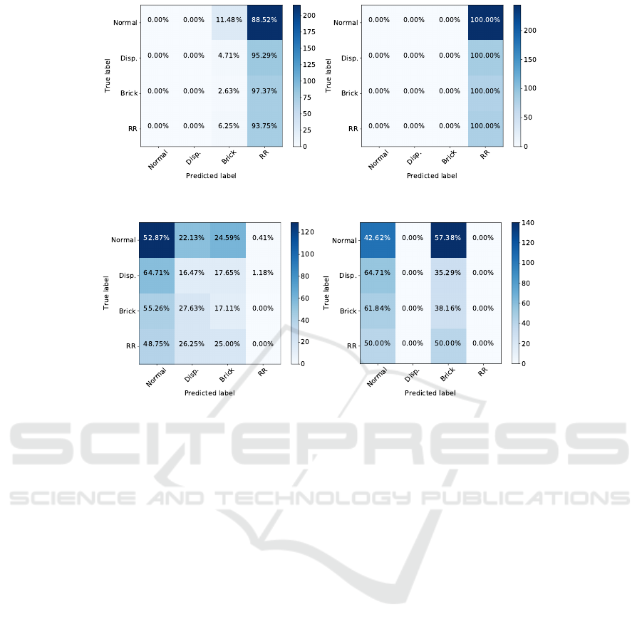
6 DISCUSSION
From the results it is evident that the DGCNN net-
work consistently outperforms the PointNet network.
Even the best performing case of PointNet, trained
using data scenario 3, which scores the highest F1
score, consistently avoids predicting the rubber rings.
This is a general theme throughout the trained Point-
Net networks, which in all other cases stick to predict-
ing one or two classes. Comparatively, the DGCNN
networks makes more well rounded predictions, with
only DGCNN-S2 consistently predicting a single
VISAPP 2021 - 16th International Conference on Computer Vision Theory and Applications
896

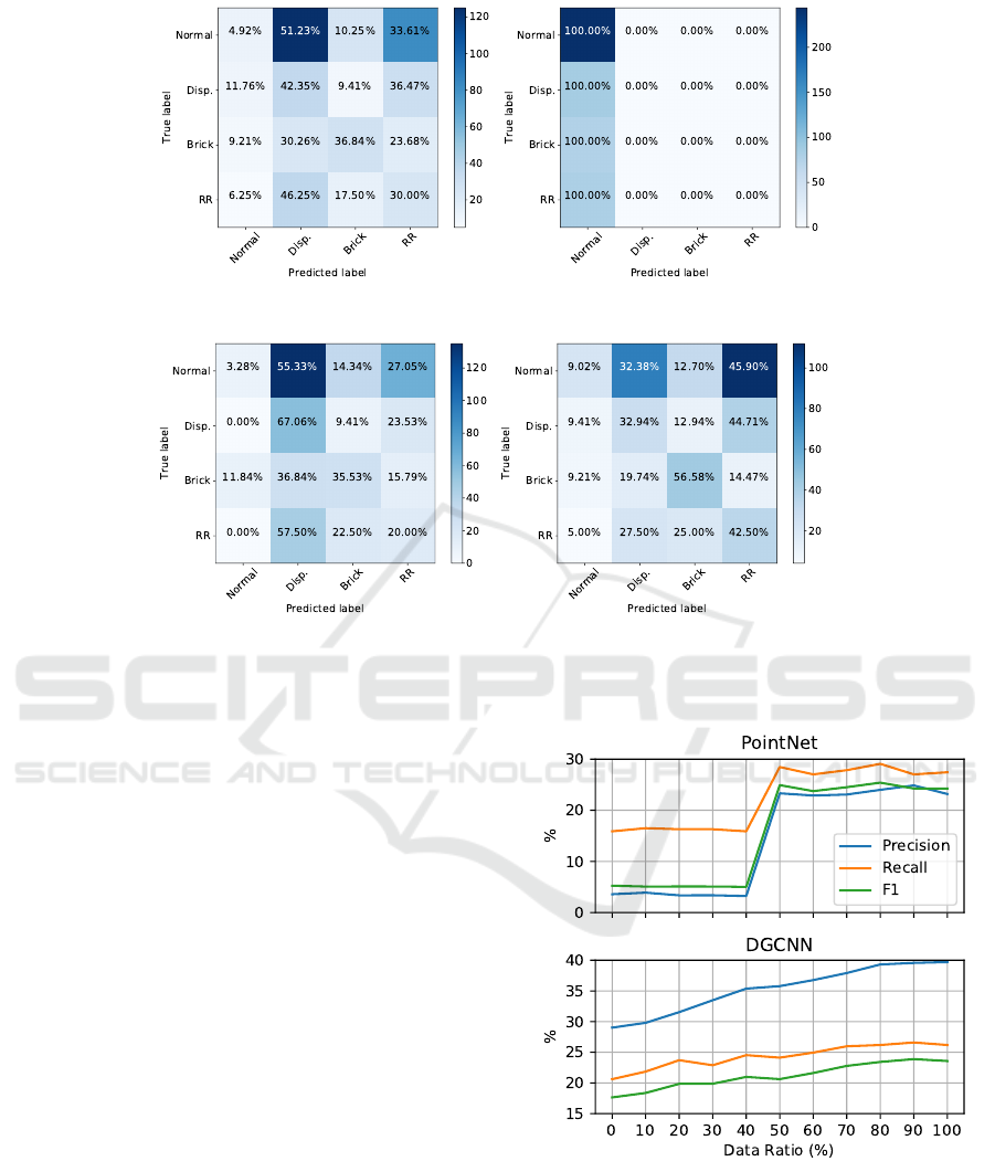
(a) DGCNN-S1 (b) DGCNN-S2
(c) DGCNN-S3 (d) DGCNN-S4
Figure 7: Confusion matrices of the real data test split, for the DGCNN architecture and four data scenarios. Disp. and RR
denotes Displacement and Rubber Ring. respectively.
class. This is reflected by the consistently high met-
rics. Therefore, it appears that there is a clear benefit
of the EdgeConv layers for the sewer defect classifi-
cation task. This makes sense as both the local and the
global structure is affected by defects, due to shadow-
ing of the sensor and changes to the pipe itself.
When looking into the different data strategies, it
is found that using either only synthetic or real data
is a poor strategy. Instead the best results were ob-
tained by pre-training on synthetic data, followed by
fine-tuning on real data. This led to a consistent im-
provement over both data scenario 1 and 3 on the real
data. Looking at Figure 6, we see that the ratio of real
point cloud data used to fine-tune the DGCNN net-
work is proportional to the metric performance. How-
ever, the PointNet network again converges to a point
where only one or two classes are predicted, as seen in
Figure 8(d). We can therefore conclude that synthetic
training data can be used to bootstrap the training pro-
cess of a 3D sewer defect classifier.
However, the networks are not a perfect classifier,
as there are several failure points. As mentioned ear-
lier, only one of the PointNets managed to converge
to a usable classifier, with the rest instead simply pre-
dicting one or two classes. Conversely, the DGCNN
converge to a more usable classifier. However, the
Figure 6: Plot of the evaluation metrics, when increasing the
ratio of the real training data used to fine-tune the networks.
best performing model, DGCNN-S4, is biased to-
wards the defect classes, with only 9% correctly pre-
dicted non-defective pipes in the real data. This may
be due to some defects occurring quite far into the
pipe, though still visible to the sensor. In these cases
Sewer Defect Classification using Synthetic Point Clouds
897

(a) PointNet-S1 (b) PointNet-S2
(c) PointNet-S3 (d) PointNet-S4
Figure 8: Confusion matrices of the real data test split, for the PointNet architecture and four data scenarios. Disp. and RR
denotes Displacement and Rubber Ring. respectively.
the effect on the recorded point cloud, such as shad-
owing, will be quite subtle, and more easily confused
with a normal sewer pipe.
7 CONCLUSION
In this work we investigate the possibility of utilizing
modern geometric deep learning techniques in order
to detect defects in sewer pipes, using a combination
of synthetic and real point cloud data. We compare
two network architectures, PointNet and DGCNN, on
a new publicly available dataset with 17,000 point
clouds and four classes. The dataset is structured
such that the majority of the training and validation
splits consist of synthetic data, with the majority of
the point cloud data of real sewer pipes are reserved
for the test data. We conduct a grid search for the hy-
perparameters, and train the chosen networks under
four different training data scenarios, in order to in-
vestigate the effect of using synthetic and real training
data. We find that the DGCNN networks consistently
outperforms the PointNet baseline, when investigat-
ing the confusion matrices and metrics. We also find
that the best performance is achieved using both syn-
thetic and real training data, specifically when using
the real data to fine-tune a network trained on syn-
thetic data. The trained classifiers are, however, not
perfect, as they tend to favor classifying defects in-
stead of normal pipes. With these findings we show
that both geometric deep learning methods and syn-
thetic training data is viable for training sewer defect
classifiers, though more work is needed for the classi-
fiers to become more stable.
ACKNOWLEDGEMENTS
This work is supported by Innovation Fund Denmark
[grant number 8055-00015A] and is part of the Auto-
mated Sewer Inspection Robot (ASIR) project. The
authors declare no conflict of interests.
REFERENCES
Ahrary, A., Kawamura, Y., and Ishikawa, M. (2006). A
laser scanner for landmark detection with the sewer
inspection robot kantaro. In 2006 IEEE/SMC Interna-
tional Conference on System of Systems Engineering.
VISAPP 2021 - 16th International Conference on Computer Vision Theory and Applications
898

Alejo, D., Caballero, F., and Merino, L. (2017). Rgbd-
based robot localization in sewer networks. In
2017 IEEE/RSJ International Conference on Intelli-
gent Robots and Systems (IROS).
Alejo, D., Mier, G., Marques, C., Caballero, F., Merino, L.,
and Alvito, P. (2020). SIAR: A Ground Robot Solution
for Semi-autonomous Inspection of Visitable Sewers.
Springer International Publishing, Cham.
American Society of Civil Engineers (2017).
2017 infrastructure report card - wastewater.
https://www.infrastructurereportcard.org/wp-content/
uploads/2017/01/Wastewater-Final.pdf. Accessed:
14-11-2020.
Barnett, V. and Lewis, T. (1984). Outliers in Statistical
Data. Wiley Series in Probability and Statistics. Wi-
ley.
Beery, S., Liu, Y., Morris, D., Piavis, J., Kapoor, A., Meis-
ter, M., Joshi, N., and Perona, P. (2020). Synthetic
examples improve generalization for rare classes. In
2020 IEEE Winter Conference on Applications of
Computer Vision (WACV).
Bronstein, M. M., Bruna, J., LeCun, Y., Szlam, A., and Van-
dergheynst, P. (2017). Geometric deep learning: Go-
ing beyond euclidean data. IEEE Signal Processing
Magazine, 34(4).
CamBoard (2018). Development kit brief camboard pico
flexx. https://pmdtec.com/picofamily/wp-content/
uploads/2018/03/PMD DevKit Brief CB pico flexx
CE V0218-1.pdf. Accessed: 25-11-2020.
Cao, W., Yan, Z., He, Z., and He, Z. (2020). A comprehen-
sive survey on geometric deep learning. IEEE Access,
8.
Car, M., Markovic, L., Ivanovic, A., Orsag, M., and Bog-
dan, S. (2020). Autonomous wind-turbine blade in-
spection using lidar-equipped unmanned aerial vehi-
cle. IEEE Access, 8.
Duran, O., Althoefer, K., and Seneviratne, L. D. (2003).
Pipe inspection using a laser-based transducer and au-
tomated analysis techniques. IEEE/ASME Transac-
tions on Mechatronics, 8(3).
Duran, O., Althoefer, K., and Seneviratne, L. D. (2004).
Automated pipe inspection using ann and laser data
fusion. In IEEE International Conference on Robotics
and Automation, 2004. Proceedings. ICRA ’04. 2004,
volume 5.
Duran, O., Althoefer, K., and Seneviratne, L. D. (2007).
Automated pipe defect detection and categorization
using camera/laser-based profiler and artificial neural
network. IEEE Transactions on Automation Science
and Engineering, 4(1).
Garrido, G. G., Sattar, T., Corsar, M., James, R., and
Seghier, D. (2018). Towards safe inspection of long
weld lines on ship hulls using an autonomous robot. In
21st International Conference on Climbing and Walk-
ing Robots.
Hassan, S. I., Dang, L. M., Mehmood, I., Im, S., Choi, C.,
Kang, J., Park, Y.-S., and Moon, H. (2019). Under-
ground sewer pipe condition assessment based on con-
volutional neural networks. Automation in Construc-
tion, 106.
Haurum, J. B. and Moeslund, T. B. (2020). A survey on
image-based automation of cctv and sset sewer in-
spections. Automation in Construction, 111.
Henriksen, K. S., Lynge, M. S., Jeppesen, M. D. B., Al-
lahham, M. M. J., Nikolov, I. A., Haurum, J. B., and
Moeslund, T. B. (2020). Generating synthetic point
clouds of sewer networks: An initial investigation.
In Augmented Reality, Virtual Reality, and Computer
Graphics, Cham. Springer International Publishing.
Iyer, S., Sinha, S. K., Pedrick, M. K., and Tittmann, B. R.
(2012). Evaluation of ultrasonic inspection and imag-
ing systems for concrete pipes. Automation in Con-
struction, 22. Planning Future Cities-Selected papers
from the 2010 eCAADe Conference.
Khan, M. S. and Patil, R. (2018a). Acoustic characterization
of pvc sewer pipes for crack detection using frequency
domain analysis. In 2018 IEEE International Smart
Cities Conference (ISC2).
Khan, M. S. and Patil, R. (2018b). Statistical analysis of
acoustic response of pvc pipes for crack detection. In
SoutheastCon 2018.
Kolesnik, M. and Baratoff, G. (2000). Online distance
recovery for a sewer inspection robot. In Proceed-
ings 15th International Conference on Pattern Recog-
nition. ICPR-2000, volume 1.
Kumar, S. S., Wang, M., Abraham, D. M., Jahanshahi,
M. R., Iseley, T., and Cheng, J. C. P. (2020). Deep
learning–based automated detection of sewer
defects in cctv videos. Journal of Computing in Civil
Engineering, 34(1).
Lang, A. H., Vora, S., Caesar, H., Zhou, L., Yang, J.,
and Beijbom, O. (2019). Pointpillars: Fast encoders
for object detection from point clouds. In 2019
IEEE/CVF Conference on Computer Vision and Pat-
tern Recognition (CVPR).
Lepot, M., Stani
´
c, N., and Clemens, F. H. (2017). A tech-
nology for sewer pipe inspection (part 2): Experimen-
tal assessment of a new laser profiler for sewer defect
detection and quantification. Automation in Construc-
tion, 73.
Li, D., Cong, A., and Guo, S. (2019). Sewer damage detec-
tion from imbalanced cctv inspection data using deep
convolutional neural networks with hierarchical clas-
sification. Automation in Construction, 101.
Loshchilov, I. and Hutter, F. (2017). SGDR: stochastic gra-
dient descent with warm restarts. In 5th International
Conference on Learning Representations, ICLR 2017,
Toulon, France, April 24-26, 2017, Conference Track
Proceedings. OpenReview.net.
Menendez, E., Victores, J. G., Montero, R., Mart
´
ınez, S.,
and Balaguer, C. (2018). Tunnel structural inspection
and assessment using an autonomous robotic system.
Automation in Construction, 87.
Myrans, J., Everson, R., and Kapelan, Z. (2018). Auto-
mated detection of faults in sewers using cctv image
sequences. Automation in Construction, 95.
Nasrollahi, M., Bolourian, N., and Hammad, A. (2019).
Concrete surface defect detection using deep neural
network based on lidar scanning. In Proceedings of
Sewer Defect Classification using Synthetic Point Clouds
899

the CSCE Annual Conference, Laval, Greater Mon-
treal, QC, Canada.
Nielsen, M. S., Nikolov, I., Kruse, E. K., Garnæs, J., and
Madsen, C. B. (2020). High-resolution structure-
from-motion for quantitative measurement of leading-
edge roughness. Energies, 13(15).
Pham, N. H., La, H. M., Ha, Q. P., Dang, S. N., Vo, A. H.,
and Dinh, Q. H. (2016). Visual and 3d mapping for
steel bridge inspection using a climbing robot. In IS-
ARC 2016-33rd International Symposium on Automa-
tion and Robotics in Construction.
Prakash, A., Boochoon, S., Brophy, M., Acuna, D., Cam-
eracci, E., State, G., Shapira, O., and Birchfield, S.
(2019). Structured domain randomization: Bridging
the reality gap by context-aware synthetic data. In
2019 International Conference on Robotics and Au-
tomation (ICRA).
Qi, C. R., Su, H., Mo, K., and Guibas, L. J. (2017a). Point-
net: Deep learning on point sets for 3d classification
and segmentation. In 2017 IEEE Conference on Com-
puter Vision and Pattern Recognition (CVPR).
Qi, C. R., Su, H., Nießner, M., Dai, A., Yan, M., and
Guibas, L. J. (2016). Volumetric and multi-view cnns
for object classification on 3d data. In 2016 IEEE
Conference on Computer Vision and Pattern Recog-
nition (CVPR).
Qi, C. R., Yi, L., Su, H., and Guibas, L. J. (2017b). Point-
net++: Deep hierarchical feature learning on point sets
in a metric space. In Advances in Neural Information
Processing Systems 30. Curran Associates, Inc.
Qin, X., Wu, G., Lei, J., Fan, F., Ye, X., and Mei, Q. (2018).
A novel method of autonomous inspection for trans-
mission line based on cable inspection robot lidar data.
Sensors, 18(2).
Ravi, R., Bullock, D., and Habib, A. (2020). Highway and
airport runway pavement inspection using mobile li-
dar. The International Archives of Photogrammetry,
Remote Sensing and Spatial Information Sciences, 43.
Rousseeuw, P. J. and Leroy, A. M. (2005). Robust regres-
sion and outlier detection, volume 589. John wiley &
sons.
Santur, Y., Karak
¨
ose, M., and Akın, E. (2016). Condition
monitoring approach using 3d modelling of railway
tracks with laser cameras. In International Conference
on Advanced Technology & Sciences (ICAT’16) pp.
Sinha, S. K. and Fieguth, P. W. (2006a). Automated de-
tection of cracks in buried concrete pipe images. Au-
tomation in Construction, 15(1).
Sinha, S. K. and Fieguth, P. W. (2006b). Neuro-fuzzy net-
work for the classification of buried pipe defects. Au-
tomation in Construction, 15(1).
Sinha, S. K. and Fieguth, P. W. (2006c). Segmentation of
buried concrete pipe images. Automation in Construc-
tion, 15(1).
Su, H., Maji, S., Kalogerakis, E., and Learned-Miller, E.
(2015). Multi-view convolutional neural networks for
3d shape recognition. In 2015 IEEE International
Conference on Computer Vision (ICCV).
Su, T.-C., Yang, M.-D., Wu, T.-C., and Lin, J.-Y. (2011).
Morphological segmentation based on edge detection
for sewer pipe defects on cctv images. Expert Systems
with Applications, 38(10).
Tezerjani, A. D., Mehrandezh, M., and Paranjape, R.
(2015). Defect detection in pipes using a mobile laser-
optics technology and digital geometry. MATEC Web
of Conferences, 32.
Tobin, J., Fong, R., Ray, A., Schneider, J., Zaremba, W., and
Abbeel, P. (2017). Domain randomization for transfer-
ring deep neural networks from simulation to the real
world. In 2017 IEEE/RSJ International Conference
on Intelligent Robots and Systems (IROS).
Vora, S., Lang, A. H., Helou, B., and Beijbom, O. (2020).
Pointpainting: Sequential fusion for 3d object detec-
tion. In 2020 IEEE/CVF Conference on Computer Vi-
sion and Pattern Recognition (CVPR).
Wang, M. and Cheng, J. C. P. (2020). A unified convolu-
tional neural network integrated with conditional ran-
dom field for pipe defect segmentation. Computer-
Aided Civil and Infrastructure Engineering, 35(2).
Wang, Y., Chao, W., Garg, D., Hariharan, B., Campbell, M.,
and Weinberger, K. Q. (2019). Pseudo-lidar from vi-
sual depth estimation: Bridging the gap in 3d object
detection for autonomous driving. In 2019 IEEE/CVF
Conference on Computer Vision and Pattern Recogni-
tion (CVPR).
Wang, Y., Sun, Y., Liu, Z., Sarma, S. E., Bronstein, M. M.,
and Solomon, J. M. (2019). Dynamic graph cnn for
learning on point clouds. ACM Trans. Graph., 38(5).
Wen, X., Song, K., Niu, M., Dong, Z., and Yan, Y. (2017). A
three-dimensional inspection system for high temper-
ature steel product surface sample height using stereo
vision and blue encoded patterns. Optik, 130.
Wu, W., Liu, Z., and He, Y. (2013). Classification of de-
fects with ensemble methods in the automated visual
inspection of sewer pipes. Pattern Analysis and Ap-
plications, 18(2).
Yang, M.-D. and Su, T.-C. (2008). Automated diagnosis
of sewer pipe defects based on machine learning ap-
proaches. Expert Systems with Applications, 35(3).
Zhou, Y. and Tuzel, O. (2018). Voxelnet: End-to-end learn-
ing for point cloud based 3d object detection. In 2018
IEEE/CVF Conference on Computer Vision and Pat-
tern Recognition.
VISAPP 2021 - 16th International Conference on Computer Vision Theory and Applications
900