Are Image Patches Beneﬁcial for Initializing Convolutional Neural

Network Models?

Daniel Lehmann and Marc Ebner

Institut f

ur Mathematik und Informatik, Universit

at Greifswald,

Walther-Rathenau-Straße 47, 17489 Greifswald, Germany

Keywords:

Convolutional Neural Network, Neural Network Weight Initialization.

Abstract:

Before a neural network can be trained the network weights have to be initialized somehow. If a model is

trained from scratch, current approaches for weight initialization are based on random values. In this work

we examine another approach to initialize the weights of convolutional neural network models for image

classiﬁcation. Our approach relies on presetting the weights of convolutional layers based on information given

in the training images. To initialize the weights of convolutional layers we use small patches extracted from the

training images to preset the ﬁlters of the convolutional layers. Experiments conducted on the MNIST, CIFAR-

10 and CIFAR-100 dataset show that using image patches for the network initialization performs similar to

state-of-the-art initialization approaches. The advantage is that our approach is more robust with respect to

the learning rate. When a suboptimal value for the learning rate is used for training, our approach performs

slightly better than current approaches. As a result, information given in the training images seems to be useful

for network initialization resulting in a more robust training process.

1 INTRODUCTION

Neural network models are widely used for image

classiﬁcation. However, training such models from

scratch is a non-trivial task. The goal of training

is to ﬁnd model weights that result in minimal loss

for the corresponding classiﬁcation task. Unfortu-

nately, it is not obvious which weight values work

best. We need to ﬁnd optimal values through iterative

optimization (usually based on stochastic gradient de-

scent). We start with an initial value for each weight

and gradually adjust these values over multiple itera-

tions (Robbins and Monro, 1951; Ruder, 2016). The

crucial steps in this process are: 1) How should we

set the initial weights? 2) How can we update the

weights in each iteration? In this work we focus on

the ﬁrst question. Ideally, the initial weights should

be set as close as possible to the optimal weights

to avoid a large number of training iterations. This

way we reduce training time and decrease the risk of

getting stuck in local minima or saddle points dur-

ing the training process. But how can we ﬁnd good

initial weight values when we want to train a model

from scratch? State-of-the-art (SOTA) methods for

initializing model weights are based on random val-

ues (Glorot and Bengio, 2010; He et al., 2015b).

However, SOTA approaches to train a model from

scratch can still take a long time. To speed up train-

ing we may replace certain network layers in a way

that simpliﬁes the training process. Ideally, we do

not want to adjust the weights of these layers at all

or only slightly once they have been set. If this is pos-

sible, then we move towards explainable neural net-

work computation as opposed to black box training.

Model explainability leads to increased trust in the ﬁ-

nal models. This is particularly important for safety-

critical applications (e.g., autonomous driving, medi-

cal applications). Hence, explainability of neural net-

work models is an important area of current research

(Angelov and Soares, 2019; Li et al., 2017; Xie et al.,

2020).

In our work we also take a ﬁrst step in this direc-

tion. We focus on an alternative approach to initialize

convolutional neural network (CNN) models for im-

age classiﬁcation. We examine whether it is beneﬁcial

to use information given by the training images to ini-

tialize the network weights. To initialize the weights

of a convolutional layer (ConvLayer) we use small

patches extracted from the training images to preset

each ﬁlter of the ConvLayer. Using this approach we

state the following research questions: 1) Does this

approach allow model training or does it destroy the

346

Lehmann, D. and Ebner, M.

Are Image Patches Beneﬁcial for Initializing Convolutional Neural Network Models?.

DOI: 10.5220/0010206603460353

In Proceedings of the 16th International Joint Conference on Computer Vision, Imaging and Computer Graphics Theory and Applications (VISIGRAPP 2021) - Volume 5: VISAPP, pages

346-353

ISBN: 978-989-758-488-6

training process? 2) If it does allow training, will it

also reach or even surpass the classiﬁcation accuracy

of models initialized with SOTA initialization meth-

ods? We have found that initializing network weights

using image patches does allow a reasonable training

process. This approach even reaches a similar clas-

siﬁcation performance compared to SOTA initializa-

tion methods. Furthermore, we have also observed

that an image patch based weight initialization can

make model training more robust when using subop-

timal training hyper-parameters. The remaining sec-

tions of this work are structured in the following way:

In section 2 we give an overview of current methods

to initialize CNN based models for image classiﬁca-

tion. Our approach is described in section 3. The

experiments that we have conducted as well as their

results are illustrated in section 4. In section 5 we

discuss our ﬁndings and conclude our study.

2 RELATED WORK

SOTA initialization approaches to train neural net-

work models from scratch are based on random val-

ues. Xavier and Bengio (Glorot and Bengio, 2010)

introduced Xavier initialization. Xavier picks each

weight value from a uniform distribution within an in-

terval around zero. The bounds of that interval are cal-

culated using the number of incoming and outgoing

connections of the network layer to which the weight

belongs. Xavier and Bengio conducted experiments

on neural networks using hyperbolic tangent and soft-

sign activation functions. He et al. (He et al., 2015b)

introduced Kaiming initialization. Kaiming turned

out to work better for modern neural networks us-

ing ReLU activation functions. To initialize a weight,

Kaiming picks a random value from a normal distri-

bution. The standard deviation of this normal dis-

tribution is determined by the number of incoming

connections of the network layer to which the weight

belongs. The chosen random value is used as the

initial value for that weight. Zhang et al. (Zhang

et al., 2019) introduced Fixup, which is an initializa-

tion method for deep residual networks (ResNet) (He

et al., 2015a). FixUp uses either Xavier or Kaiming

initialization plus a special scaling to set the weights

of the residual branches of the network. This special

scaling is important to prevent exploding gradients

during model training. Thus, Fixup is an alternative to

normalization layers (Ioffe and Szegedy, 2015). How-

ever, in contrast to our approach Xavier, Kaiming and

Fixup rely on random values. They do not use any

information given in the training data to initialize the

network weights as our approach does.

Another approach to initialize a neural network

model is to use the weights of a pre-trained model.

Weights of pre-trained models usually contain useful

information. Pre-trained models are obtained through

transfer learning (Zhuang et al., 2019), unsupervised

learning (Bengio et al., 2007), self-supervised learn-

ing (He et al., 2019; Misra and van der Maaten,

2019) or network pruning (Frankle and Carbin, 2018).

However, in contrast to initializing a model with the

weights of a pre-trained model we focus on weight

initialization to train a model from scratch.

Besides these SOTA approaches, a number of

other approaches to initialize neural network weights

have been proposed. For instance, a method using

sparse weight matrices (Gray et al., 2017), an or-

thogonal matrix initialization (Mishkin and Matas,

2015; Saxe et al., 2013), a method using high-pass

ﬁlters for network initialization (Castillo Camacho

and Wang, 2019), an initialization approach based

on meta-learning (Dauphin and Schoenholz, 2019),

a PCA based initialization (Seuret et al., 2017) or

a method using Gabor ﬁlters (

Ozbulak and Ekenel,

2018). However, the most similar methods to ours

also follow a data-dependent approach. Kr

ahenb

uhl

et al. (Kr

ahenb

uhl et al., 2015) proposed a method to

initialize the weights using the initial layer activations

of the training images. Koturwar and Merchant (Ko-

turwar and Merchant, 2017) suggested to use training

data statistics for weight initialization. However, in

contrast to our approach both do not use the image

data directly to initialize the weights.

3 METHOD

A CNN consists of a stack of multiple ConvLayers.

Each ConvLayer has several ﬁlters which contain the

weights of that layer. Each ﬁlter is responsible for de-

tecting a speciﬁc kind of feature in the image. Fil-

ters of the lower ConvLayers detect low level fea-

tures, whereas ﬁlters of deeper ConvLayers detect

high level features (Zeiler and Fergus, 2013). How

many ﬁlters are required for each ConvLayer depends

on the classiﬁcation problem we try to solve. A ﬁl-

ter is a 3-dimensional tensor that consists of multiple

2-dimensional slices. Each slice corresponds to a cer-

tain channel of either the input image (ﬁrst layer) or

the layer activations (all remaining layers). If there is

only one channel (e.g., grayscale input image), each

ﬁlter will just consist of a single slice (the ﬁlter be-

comes 2-dimensional). The ﬁlter slices usually have

a size of 3x3, 5x5 or 7x7 (ﬁlter size).

To initialize the ﬁlters of a ConvLayer, we use

information that is available in the training images.

Are Image Patches Beneﬁcial for Initializing Convolutional Neural Network Models?

347

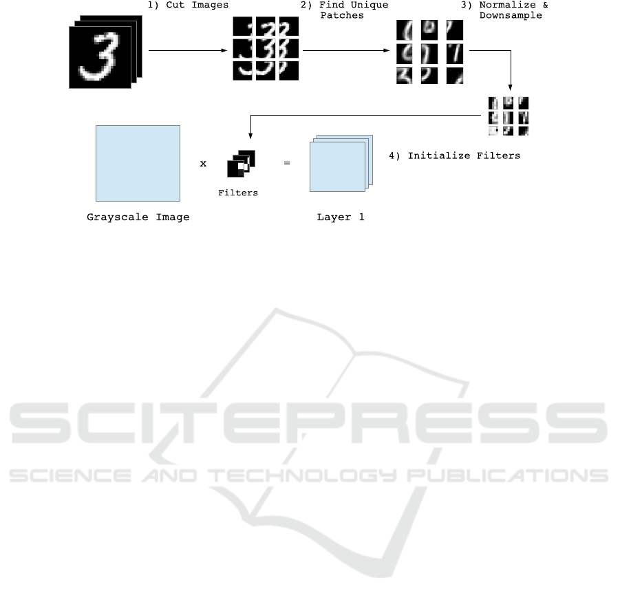
Figure 1: Our approach applied to the ﬁlters of the ﬁrst ConvLayer (MNIST): 1) Cut training images into patches. 2) Find N

unique patches using k-Means (N = number of ﬁlters). 3) Normalize and downsample identiﬁed patches to the ﬁlter size. 4)

Initialize the ﬁlters with the patches.

For our initial experiments, we have used grayscale

images of handwritten digits of size 28x28 pixel

from the MNIST dataset (LeCun and Cortes, 1998).

We take the MNIST training images and cut them

into multiple patches of the same size. Neighbor-

ing patches of an image should overlap up to a cer-

tain amount to retain as much information as possible

from each image. We choose one of the MNIST im-

ages to explain how the patches are created for initial-

izing the ﬁlters of the ﬁrst ConvLayer. An intuitive

approach is to cut the MNIST image into patches of

the appropriate ﬁlter size (e.g., 5x5). However, our

experiments have shown that cutting the image into

patches bigger than the ﬁlter size followed by down-

sampling these patches to the required ﬁlter size has

a beneﬁcial effect on model training. For instance,

we choose a patch size of 14x14 pixel with an over-

lap of 7 pixel for neighboring patches. After cutting

the image apart, we obtain 9 of those patches. An il-

lustration of this process is shown in step 1 in ﬁgure

1. However, it is possible that some of the patches do

not contain a lot of information. For instance, some of

the MNIST patches might almost only show the black

background of the image. Obviously, such patches

are not useful for model training. Thus, we remove

all patches that contain less than 20 non-black pixels.

All of the remaining patches should have a sufﬁcient

amount of information. These patches should be used

to initialize the ﬁlters of the ﬁrst ConvLayer.

Applying this procedure to all training images

results in an exceedingly large number of patches.

However, the number of ﬁlters of the layer is quite

small. If the ConvLayer has 20 ﬁlters for instance, we

need to select 20 of those patches to initialize each

of the 20 ﬁlters with a patch. Obviously, the chosen

patches should be as unique as possible to avoid ini-

tializing all ﬁlters with similar patches. To ﬁnd unique

patches we use k-Means clustering (Kanungo et al.,

2002). We unroll each 2-dimensional patch to a vec-

tor and stack all of these vectors together resulting in a

matrix of size (number of patches) x (number of patch

pixels). Since it is rather difﬁcult to apply k-Means

to high-dimensional spaces, we use UMAP (McInnes

et al., 2018) to that matrix to reduce its size to (num-

ber of patches) x 2. Finally, we apply k-Means with

k = 20 to identify 20 clusters. Then we take the 10

closest patches from each of the 20 cluster centers,

reshape the pixel values back to two dimensions and

average these 10 patches for each cluster center. This

way we do not rely only on a single image patch but

on a mean image patch for each cluster center. These

mean image patches are used for ﬁlter initialization.

Before we can initialize the ﬁlters, we need to ap-

ply two additional preprocessing steps to the iden-

tiﬁed 20 patches. As a ﬁrst preprocessing step we

need to normalize each patch to have zero mean. Our

experiments have shown that normalizing patches to

zero mean has a beneﬁcial effect on model training.

This corresponds to SOTA initialization methods us-

ing random values, which also pick initial weight val-

ues from a distribution around zero. In a second

preprocessing step we have to adjust the size of the

patches to the ﬁlter size of the ConvLayer. In our ex-

ample we cut an MNIST image into patches of size

14x14 pixel. If the ﬁlter size of the ﬁrst ConvLayer

is 5x5, we need to downsample the patches of size

14x14 to a size of 5x5 pixel. After downsampling,

the patches are ready to be used for initializing the

ﬁlters of the ConvLayer. Thus, we stack all created

patches together and use the resulting 3-dimensional

tensor of size 20x5x5 as the initial ﬁlter values of the

ﬁrst ConvLayer. In the same way we can also ini-

VISAPP 2021 - 16th International Conference on Computer Vision Theory and Applications

348

tialize the ﬁlter values of the other ConvLayers. After

initialization, we can train the model in the usual way.

Figure 2: Example Patches extracted from CIFAR-10 using

SIFT and k-Means.

For our experiments using color images of size

32x32 pixel of the CIFAR-10 and CIFAR-100 dataset

(Krizhevsky and Hinton, 2009) we have used almost

the same approach as described above. However, we

do not cut the whole image into patches. Instead,

we look for characteristic keypoints in the image us-

ing the SIFT keypoint detector (Lowe, 2004) and cut

out the patches around each detected keypoint (e.g.,

patches of size 15x15 pixel). This way we should only

obtain image patches containing a sufﬁcient amount

of information. Furthermore, due to computational

limitations we use PCA (Pearson, 1901) for dimen-

sionality reduction. Finally, after clustering we only

select the closest patch to each cluster center to avoid

averaging patches containing different backgrounds

which would result into washed out image patches.

4 EXPERIMENTS

4.1 Comparison to the State-of-the-Art

We have conducted an experiment to ﬁnd out whether

initializing model weights with image patches (as de-

scribed in section 3) is useful at all. In this case

it should be possible to train a model at least for

MNIST. Thus, we have chosen to train such a model

ﬁrst of all. Furthermore, we have compared the train-

ing process of that model to the training process of

models using the following SOTA approaches: the

original Kaiming initialization using a normal distri-

bution (Kaiming Normal) and a Kaiming initializa-

tion using a uniform distribution (Kaiming Uniform,

which is the standard initialization method in Py-

Torch

). As model network architecture we have used

the Caffe LeNet architecture

, since it is a standard ar-

https://pytorch.org/docs/stable/nn.init.html

https://github.com/BVLC/caffe/tree/master/examples/

mnist

chitecture for MNIST. We have initialized the weights

of the ﬁrst ConvLayer (20 ﬁlters, ﬁlter size: 5x5)

using image patches as described in section 3. The

weights of the other layers were initialized with the

Kaiming Uniform initialization method (standard Py-

Torch initialization method

). For model training we

used the hyper-parameter values of the Caffe LeNet

training (learning rate: 0.01, momentum: 0.9, weight

decay: 0.0005). All training and test images were

normalized before training using the MNIST statis-

tics (mean: 0.1307; std: 0.3081). We have trained

5 models for each initialization approach: our patch

based approach applied to the ﬁrst ConvLayer, Kaim-

ing Uniform and Kaiming Normal. For each of the

5 models using our approach we have used a differ-

ent seed value to obtain various weight initializations

based on Kaiming Uniform for the other layers be-

sides the ﬁrst layer. For comparison we have used

the same seed values for the 5 models using Kaim-

ing Uniform and the 5 models using Kaiming Normal.

After each training epoch we recorded the mean and

standard deviation of the obtained accuracies of the 5

models of each approach on the test set. Each model

was trained for 20 epochs. The results of our experi-

ment are illustrated in ﬁgure 3 (top left). The obtained

test accuracies of our approach are quite similar to

the accuracies obtained by the models initialized with

Kaiming Uniform and Kaiming Normal after each

training epoch. There is even a slight improvement

of our approach compared to Kaiming Normal.

However, MNIST is a quite simple classiﬁcation

problem. Thus, we have also tested how initializ-

ing model weights with image patches inﬂuences the

training process for the CIFAR-10 dataset in compar-

ison to the FixUp initialization. As model network

architecture we have used the same 20-layer ResNet

(He et al., 2015a) that was also used by Zhang et al.

(Zhang et al., 2019). The network has 268,393 train-

able parameters. We initialized the 16 ﬁlters of the

ﬁrst ConvLayer (ﬁlter tensor size: 3x3x3) using im-

age patches as described in section 3. We have cut out

patches of size 15x15x3 pixel around each detected

SIFT keypoint. Then, we have identiﬁed 16 unique

patches using k-Means (for the 16 ﬁlters of the ﬁrst

ConvLayer). Finally, the 16 patches were normal-

ized and downsampled to a size of 3x3x3. The result-

ing patches were stacked together to a tensor of size

16x3x3x3. This tensor was used as initial ﬁlter tensor

for the ﬁrst ConvLayer. The weights of the other lay-

ers were initialized with FixUp. For model training

we used the same hyper-parameter values

that were

also used by Zhang et al. (Zhang et al., 2019) (initial

learning rate: 0.1, cosine annealing schedule for the

https://github.com/hongyi-zhang/Fixup

Are Image Patches Beneﬁcial for Initializing Convolutional Neural Network Models?

349

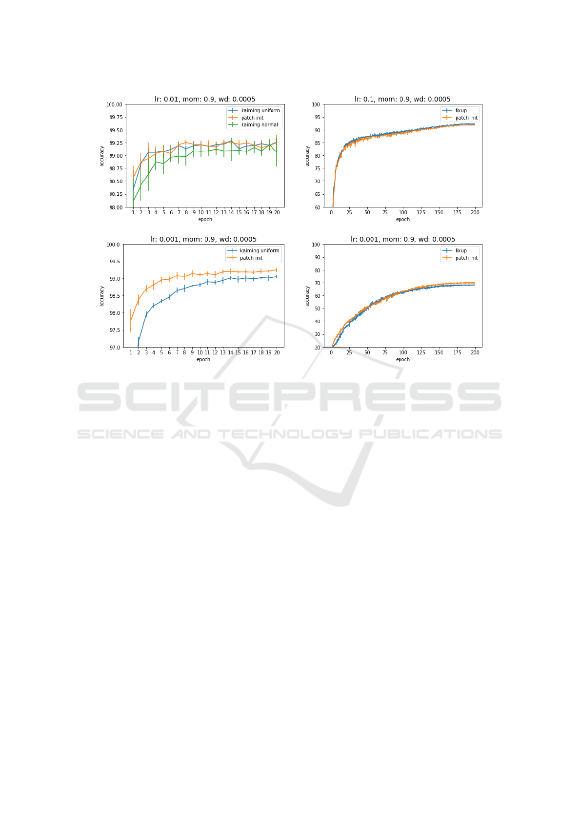
MNIST

CIFAR-10

Figure 3: Model performance of our approach compared to SOTA initialization for MNIST (left) and CIFAR-10 (right) using

an optimal learning rate (top) and a suboptimal learning rate (bottom). Test accuracies are averaged over 5 models.

learning rate, momentum: 0.9, weight decay: 0.0005,

epochs: 200, data augmentation). All images of the

training and test set were normalized before training

using the CIFAR-10 statistics (mean: 0.4914, 0.4822,

0.4465; std: 0.2023, 0.1994, 0.2010). We have trained

5 models using our initialization approach with a dif-

ferent seed value for each model to obtain various

weight initializations based on FixUp for the other

layers besides the ﬁrst layer. For comparison, we have

also trained 5 models using the standard FixUp initial-

ization with the same 5 seed values. The results of our

experiment are illustrated in ﬁgure 3 (top right). The

results show that our approach reaches similar perfor-

mance to the standard FixUp initialization.

4.2 Inﬂuence of Suboptimal

Hyper-parameters

In a second experiment, we have examined the inﬂu-

ence of the learning rate hyper-parameter on model

training using our approach compared to SOTA ini-

tializations. As in section 4.1 we have trained mod-

els from scratch on MNIST using the Caffe LeNet ar-

chitecture ﬁrst of all. For our approach the patches

have been created and used for the initialization of

the ﬁrst ConvLayer in the same way as in section 4.1.

Each model has been trained using the same hyper-

parameters, normalization and number of epochs as

in section 4.1 except for the learning rate. In section

4.1 we have used a learning rate of 1e-2. This learning

rate is also used in the Caffe LeNet training conﬁgu-

ration. In our second experiment we have changed

the learning rate to a value of 1e-3, 1e-4 and 1e-5 (0.1

was already too high for training). For each of these

learning rate values we have trained 5 models using a)

our approach (using a different random seed value for

each model) and b) Kaiming Uniform (using the same

5 seed values). After each epoch we have recorded

the mean and standard deviation of the 5 test accura-

cies obtained by each initialization method. The re-

sults of the experiment are shown in ﬁgure 3 (bottom

left). They show that when we lower the value of the

learning rate, the test accuracies decrease (especially

during the ﬁrst half of training). This effect is not

surprising, since we do not use a good value for the

learning rate anymore. However, the test accuracies

obtained by our approach have not dropped as much

as the test accuracies of Kaiming Uniform as shown

in the ﬁgure. The models initialized by our method

were still able to reach a more or less high test ac-

curacy. In contrast, when we have used the default

learning rate of 1e-2, the test accuracies of the models

using our initialization approach were still similar to

the test accuracies obtained by Kaiming Uniform (see

VISAPP 2021 - 16th International Conference on Computer Vision Theory and Applications

350

section 4.1). Additionally, we have conducted similar

tests using different values for momentum (0.9, 0.8,

0.7, 0.6 and 0.5) and weight decay (5e-5, 5e-4, 5e-

3 and 5e-2). We have reached similar results as for

the learning rate test. However, the gap between the

test accuracies resulting from our approach and the

test accuracies resulting from Kaiming Uniform was

not as high for a suboptimal momentum and weight

decay as it was for a suboptimal learning rate.

Next, we have tested the inﬂuence of the learning

rate on model training using our approach compared

to FixUp for the CIFAR-10 dataset. The same model

architecture as well as hyper-parameters as in section

4.1 have been used for model training except for the

learning rate value. As learning rate we have used a

value of 1e-3 instead of 0.1 as in section 4.1. The

results of the experiment are shown in ﬁgure 3 (bot-

tom right). They show that our approach performed

slightly better compared to FixUp (averaged over 5

models using different seed values). However, the ef-

fect has not been as strong as for MNIST.

4.3 Initializing Multiple Layers

In our ﬁrst two experiments (see section 4.1 and sec-

tion 4.2) we have only initialized the ﬁlters of the

ﬁrst ConvLayer using image patches. However, mod-

ern CNNs (e.g., ResNets) consist of a large num-

ber of layers. As a result, the effect of initializing

only the ﬁrst layer might be rather small. Thus, we

have examined the effect of initializing multiple lay-

ers using image patches on the training process in a

third experiment. First, we have conducted the ex-

periment on MNIST. Since Caffe LeNet has only two

ConvLayers, we initialized both using image patches.

However, initializing both ConvLayers with image

patches made the classiﬁcation performance slightly

worse compared to only initializing the ﬁrst Con-

vLayer. Next, we have conducted the experiment on

the CIFAR-10 dataset using the same 20-layer ResNet

architecture

as in section 4.1. We have tested 4 cases:

a) initializing only the ﬁrst ConvLayer using image

patches (as in section 4.1), b) initializing the ﬁrst Con-

vLayer and the last ConvLayer of the 3rd ResNet

block using image patches (16 ﬁlters of tensor size

16x3x3), c) initializing the same layers as in test case

b) and additionally initializing the last ConvLayer of

the 6th ResNet block using image patches (32 ﬁlters

of tensor size 32x3x3) and d) initializing the same lay-

ers as in test case c) and additionally initializing the

last ConvLayer of the 9th ResNet block using image

patches (64 ﬁlters of tensor size 64x3x3). The patches

have been created and used for ConvLayer initializa-

tion in the same way as in section 4.1. However,

for the ConvLayers other than the ﬁrst ConvLayer

the patches needed to be reshaped according to the

required ﬁlter tensor shape. For model training we

have used the same hyper-parameters, normalization

and number of epochs as in section 4.1 except for the

learning rate. We have examined the training process

using the optimal learning rate of 0.1 and a subopti-

mal learning rate of 1e-3 (as in section 4.2). The re-

sults of our experiment are illustrated in ﬁgure 4 (left)

(test accuracies are averaged over 5 models using dif-

ferent seed values). The results show that when using

a suboptimal learning rate the test accuracy increased

the more layers we initialized using image patches.

When using the optimal learning rate the test accu-

racies of the ﬁnal models were only slightly worse

compared to standard Fixup. However, for test cases

c) and d) the previously optimal learning rate of 0.1

was too high. Hence, model training was not possible

for all seed values in test case c) and d) anymore.

To see whether we really outperformed the stan-

dard FixUp initialization when using a suboptimal

learning rate we have conducted the Stuart Maxwell

signiﬁcance test between our model of test case b)

and the model trained with standard FixUp initializa-

tion using a suboptimal learning rate of 1e-3. The

Stuart Maxwell signiﬁcance test is a variation of the

McNemar signiﬁcance test for classiﬁcation problems

with more than 2 classes. The McNemar signiﬁcance

test has been recommended by Dietterich (Dietterich,

1998) to check whether two machine learning mod-

els are signiﬁcantly different. Our model of test case

b) and the model trained with standard FixUp initial-

ization are signiﬁcantly different with a probability

of more than 99%. We have also conducted a Stuart

Maxwell signiﬁcance test between our model of test

case b) and the model trained with standard FixUp

initialization using the optimal learning rate of 0.1 to

see whether the slightly better model performance of

standard FixUp compared to our model was statisti-

cally signiﬁcant. The slightly better performance of

standard FixUp was statistically signiﬁcant only for 2

of the 5 seed values used for model training (with a

probability of more than 90%). For the other 3 seed

values there was no statistical signiﬁcance.

We also examined whether our approach works 1)

on a different dataset and 2) with a different network

architecture. The same experiment (same network ar-

chitecture and training setup) was conducted using the

CIFAR-100 dataset. The results are shown in ﬁgure 4

(right). They show that our approach has the same

effect for the CIFAR-100 dataset as for the CIFAR-

10 dataset. Next, we have examined whether our ap-

proach reaches the same effect when using a differ-

ent network architecture for classifying the CIFAR-

Are Image Patches Beneﬁcial for Initializing Convolutional Neural Network Models?

351

CIFAR-10

CIFAR-100

Figure 4: Model performance of our approach applied to multiple layers (1 layer: test case a, 2 layers: test case b, 3 layers:

test case c, 4 layers: test case d) compared to FixUp for CIFAR-10 (left) and CIFAR-100 (right) using an optimal learning

rate (top) and a suboptimal learning rate (bottom). CIFAR-10 test accuracies are averaged over 5 models.

10 dataset. We have decided to use a standard 18-

layer ResNet architecture (containing normalization

layers), since it is a widely used network architec-

ture. The network has 11,181,642 trainable param-

eters. However, this time the effect was not as strong.

Only after carefully choosing which layers to initial-

ize with our approach we have been able to slightly

surpass the performance of Kaiming Uniform when

using a suboptimal learning rate.

Finally, we have also tested how our approach

performs for models pre-trained on ImageNet (Deng

et al., 2009). Therefore, we have used the 18-layer

ResNet architecture to train a model for the plant

seedling dataset

. However, altering the network

weights of the pre-trained network using our approach

resulted in a performance decrease.

5 CONCLUSION

Our experiments (illustrated in section 4) have shown

that information given in the training data can be

useful to initialize CNN based image classiﬁcation

https://www.kaggle.com/c/plant-seedlings-

classiﬁcation

models. We have been able to train such models

from scratch for the MNIST, CIFAR-10 and CIFAR-

100 classiﬁcation problem using an image patch

based weight initialization. The trained models have

reached a similar accuracy on the test set compared

to models initialized by SOTA initialization methods

over the course of training. When we have not used

optimized values for the training hyper-parameters

(learning rate, momentum, weight decay), the dete-

rioration of the test accuracy was lower for models

using the image patch based initialization. In con-

trast, the deterioration of the test accuracy was higher

for models whose weights have been initialized us-

ing SOTA methods. This effect could not only be ob-

served when initializing the ﬁrst ConvLayer but also

other ConvLayers although they are not directly con-

nected to the input image (from where the patches

were extracted). However, intermediate ConvLayers

are indirectly connected to the input image (since they

are high-level feature detectors) which might causes

this effect. As a result, it seems that using image

patches for weight initialization might make the train-

ing process more robust against choosing bad values

for the training hyper-parameters. This effect was

much stronger for the LeNet and the 20-layer ResNet

architecture used by Zhang et al. (Zhang et al., 2019)

VISAPP 2021 - 16th International Conference on Computer Vision Theory and Applications

352

compared to the 18-layer ResNet architecture. In

future work it could be investigated whether image

patches can be used to improve existing methods for

network initialization. This might also lead to a more

explainable training process.

REFERENCES

Angelov, P. and Soares, E. (2019). Towards explainable

deep neural networks (xdnn). ArXiv, abs/1912.02523.

Bengio, Y., Lamblin, P., Popovici, D., and Larochelle, H.

(2007). Greedy layer-wise training of deep networks.

In Sch

olkopf, B., Platt, J. C., and Hoffman, T., editors,

Advances in Neural Information Processing Systems,

volume 19, pages 153–160. MIT Press.

Castillo Camacho, I. and Wang, K. (2019). A sim-

ple and effective initialization of CNN for forensics

of image processing operations. In Proceedings of

the ACM Workshop on IH&MMSec, IH&MMSec’19,

pages 107–112, New York, NY, USA. ACM.

Dauphin, Y. N. and Schoenholz, S. (2019). Metainit: Ini-

tializing learning by learning to initialize. In Wallach,

H., Larochelle, H., Beygelzimer, A., d Alche-Buc, F.,

Fox, E., and Garnett, R., editors, Adv Neural Inf Pro-

cess Syst 32, pages 12645–12657. Curran Associates.

Deng, J., Dong, W., Socher, R., Li, L.-J., Li, K., and Fei-

Fei, L. (2009). Imagenet: A large-scale hierarchical

image database. In CVPR09, pages 248–255, Miami,

Florida. IEEE.

Dietterich, T. G. (1998). Approximate statistical tests

for comparing supervised classiﬁcation learning algo-

rithms. Neural Computation, 10(7):1895–1923.

Frankle, J. and Carbin, M. (2018). The lottery ticket hy-

pothesis: Finding sparse, trainable neural networks.

ArXiv, abs/1803.03635.

Glorot, X. and Bengio, Y. (2010). Understanding the dif-

ﬁculty of training deep feedforward neural networks.

In JMLR W&CP: Proceedings of the 13th Int Conf on

AI and Statistics, volume 9, pages 249–256.

Gray, S., Radford, A., and Kingma, D. P. (2017). GPU

kernels for block-sparse weights.

He, K., Fan, H., Wu, Y., Xie, S., and Girshick, R. (2019).

Momentum contrast for unsupervised visual represen-

tation learning. ArXiv, abs/1911.05722.

He, K., Zhang, X., Ren, S., and Sun, J. (2015a). Deep

residual learning for image recognition. ArXiv,

abs/1512.03385.

He, K., Zhang, X., Ren, S., and Sun, J. (2015b). Delving

deep into rectiﬁers: Surpassing human-level perfor-

mance on imagenet classiﬁcation. In Proceedings of

the 2015 IEEE ICCV, ICCV 2015, pages 1026–1034,

USA. IEEE Computer Society.

Ioffe, S. and Szegedy, C. (2015). Batch normalization: Ac-

celerating deep network training by reducing internal

covariate shift. ArXiv, abs/1502.03167.

Kanungo, T., Mount, D. M., Netanyahu, N. S., Piatko,

C. D., Silverman, R., and Wu, A. Y. (2002). An efﬁ-

cient k-Means clustering algorithm: Analysis and im-

plementation. IEEE PAMI, 24(7):881–892.

Koturwar, S. and Merchant, S. (2017). Weight initialization

of deep neural networks (DNNs) using data statistics.

ArXiv, 1710.10570.

ahenb

uhl, P., Doersch, C., Donahue, J., and Darrell, T.

(2015). Data-dependent initializations of convolu-

tional neural networks. ArXiv, abs/1511.06856.

Krizhevsky, A. and Hinton, G. (2009). Learning multiple

layers of features from tiny images. Master’s thesis,

Department of Computer Science, Uni of Toronto.

LeCun, Y. and Cortes, C. (1998). The MNIST database of

handwritten digits.

Li, O., Liu, H., Chen, C., and Rudin, C. (2017). Deep learn-

ing for case-based reasoning through prototypes: A

neural network that explains its predictions. ArXiv,

abs/1710.04806.

Lowe, D. G. (2004). Distinctive image features from scale-

invariant keypoints. Int J Comput Vis, 60(2):91–110.

McInnes, L., Healy, J., and Melville, J. (2018). UMAP:

Uniform manifold approximation and projection for

dimension reduction. ArXiv, 1802.03426.

Mishkin, D. and Matas, J. (2015). All you need is a good

init. ArXiv, abs/1511.06422.

Misra, I. and van der Maaten, L. (2019). Self-supervised

learning of pretext-invariant representations. ArXiv,

abs/1912.01991.

Ozbulak, G. and Ekenel, H. K. (2018). Initialization of

convolutional neural networks by gabor ﬁlters. 26th

Signal Processing and Communications Applications

Conference (SIU), pages 1–4.

Pearson, K. (1901). LIII. On lines and planes of closest ﬁt to

systems of points in space. The London, Edinburgh,

and Dublin Philosophical Magazine and Journal of

Science, 2(11):559–572.

Robbins, H. and Monro, S. (1951). A stochastic approxi-

mation method. Ann Math Stat, 22:400–407.

Ruder, S. (2016). An overview of gradient descent opti-

mization algorithms. ArXiv, abs/1609.04747.

Saxe, A. M., McClelland, J. L., and Ganguli, S. (2013). Ex-

act solutions to the nonlinear dynamics of learning in

deep linear neural networks. ArXiv, abs/1312.6120.

Seuret, M., Alberti, M., Liwicki, M., and Ingold, R. (2017).

PCA-initialized deep neural networks applied to docu-

ment image analysis. In 14th IAPR International Con-

ference on Document Analysis and Recognition (IC-

DAR), volume 01, pages 877–882.

Xie, N., Ras, G., van Gerven, M., and Doran, D. (2020).

Explainable deep learning: A ﬁeld guide for the unini-

tiated. ArXiv, abs/2004.14545.

Zeiler, M. D. and Fergus, R. (2013). Visualizing

and understanding convolutional networks. ArXiv,

abs/1311.2901.

Zhang, H., Dauphin, Y. N., and Ma, T. (2019). Fixup ini-

tialization: Residual learning without normalization.

ArXiv, abs/1901.09321.

Zhuang, F., Qi, Z., Duan, K., Xi, D., Zhu, Y., Zhu, H.,

Xiong, H., and He, Q. (2019). A comprehensive sur-

vey on transfer learning. ArXiv, abs/1512.03385.

Are Image Patches Beneﬁcial for Initializing Convolutional Neural Network Models?

353