Interpreting Convolutional Networks Trained on Textual Data

Reza Marzban

and Christopher Crick

Computer Science Department, Oklahoma State University, Stillwater, Oklahoma, U.S.A.

Keywords:

Explainable Artiﬁcial Intelligence, Natural Language Processing, Deep Learning, Artiﬁcial Neural Networks,

Convolutional Networks.

Abstract:

There have been many advances in the artiﬁcial intelligence ﬁeld due to the emergence of deep learning. In

almost all sub-ﬁelds, artiﬁcial neural networks have reached or exceeded human-level performance. However,

most of the models are not interpretable. As a result, it is hard to trust their decisions, especially in life and

death scenarios. In recent years, there has been a movement toward creating explainable artiﬁcial intelligence,

but most work to date has concentrated on image processing models, as it is easier for humans to perceive

visual patterns. There has been little work in other ﬁelds like natural language processing. In this paper, we

train a convolutional model on textual data and analyze the global logic of the model by studying its ﬁlter

values. In the end, we ﬁnd the most important words in our corpus to our model’s logic and remove the

rest (95%). New models trained on just the 5% most important words can achieve the same performance as

the original model while reducing training time by more than half. Approaches such as this will help us to

understand NLP models, explain their decisions according to their word choices, and improve them by ﬁnding

blind spots and biases.

1 INTRODUCTION

In the big data era, traditional naive statistical models

and machine learning algorithms are not able to

keep up with the growth in data complexity. Such

algorithms are the best choice when our data size is

limited and nicely shaped in tabular formats. Pre-

viously, we were interested in analyzing structured

data in databases, inserted by an expert, but now we

use machine learning in every aspect of life. Most

of the data is unstructured, such as images, text,

voice, and videos. In addition, the amount of data has

increased signiﬁcantly. Traditional machine learning

algorithms cannot handle these types of data at our de-

sired performance level. Artiﬁcial Neural Networks

(ANNs) have undergone several waves of popularity

and disillusionment stretching back to 1943. Re-

cently, due to increases in computing power and data

availability, the success and improvement of ANNs

and deep learning have been the hot topic in machine

learning conferences. In many problem areas, deep

learning has reached or surpassed human perfor-

mance, and is the current champion in ﬁelds from

https://orcid.org/0000-0003-2762-1432

https://orcid.org/0000-0002-1635-823X

image processing and object detection to Natural

Language Processing (NLP) and voice recognition.

Although deep learning has increased perfor-

mance across the board, it still has many challenges

and limitations. One main criticism of deep learning

models is that they are black boxes: we throw data

at it, use the output and hope for the best, but we do

not understand how or why. This is less likely to be

the case with traditional statistical and machine learn-

ing methods such as decision trees. Such algorithms

are interpretable and easy to understand, and we can

know the reasoning behind the decisions they make.

Explainability is very important if we want people to

rely on our models and trust their decisions. This

becomes crucial when the models’ decisions are life-

and-death situations like medicine or autonomous ve-

hicles, and it is the reason behind the trend toward ex-

plainable artiﬁcial intelligence. In addition to boost-

ing users’ trust, however, interpretability also helps

developers, experts and scientists learn the shortcom-

ings of their models, check them for bias and tune

them for further improvement.

Many papers and tools have recently contributed

to explainability in deep learning models, but most

of them have concentrated on machine vision prob-

lems, as images are easier to visualize in a 2-

196

Marzban, R. and Crick, C.

Interpreting Convolutional Networks Trained on Textual Data.

DOI: 10.5220/0010205901960203

In Proceedings of the 10th International Conference on Pattern Recognition Applications and Methods (ICPRAM 2021), pages 196-203

ISBN: 978-989-758-486-2

dimensional space. They can use segmentation and

create heatmaps to show users which pixel or object

in the image is important, and which of them caused

a speciﬁc decision. Humans can easily ﬁnd visual

patterns in a 2-dimensional space. However, there is

also a need for model interpretability in other con-

texts like NLP, the science of teaching machines to

communicate with us in human-understandable lan-

guages. As NLP data mostly consists of texts, sen-

tences and words, it is very hard to visualize in a 2-D

or 3-D space that humans can easily interpret, even

though visualization of a model is an important part

of explainable AI.

Deep learning networks have various architec-

tures. Convolutional neural networks (CNNs) were

primarily designed for image classiﬁcation but can be

applied to all types of data. Recurrent neural networks

(RNNs) are often a good choice for time-series data;

Long Short Term Memory (LSTMs) and Gated Re-

current Units (GRUs) are common forms of RNN.

Many scientists prefer to use LSTMs on NLP prob-

lems, as they are constructed with time series in mind.

Each word can be looked at as a time step in a sen-

tence. 1-dimensional CNNs can also be used on tex-

tual data. They are faster than LSTMs and perform

well on well-known NLP problems like text classiﬁ-

cation and sentiment analysis.

In this paper we have created a simple 1-D CNN

and trained it on a large labeled corpus for sentiment

analysis, which aims understand the emotion and se-

mantic content of text and predict if its valence is pos-

itive or negative. We then deconstructed and analyzed

the CNN layer ﬁlters. We tried to understand the ﬁl-

ter patterns and why the learning algorithm would

produce them. The ﬁrst result indicates that the ﬁl-

ter weights cover around 70% of a layer’s informa-

tion, while their order covers only 30%. As a result,

randomly shufﬂing ﬁlters causes a particular layer to

lose 30% of the accuracy contributed by a particular

layer. We also used activation maximization to cre-

ate an equation to ﬁnd the importance of each word

in our corpus dictionary to the whole model. This im-

portance rate is not speciﬁc to a single decision but

to the whole model logic. We were able to order the

word corpus according to their decision-making util-

ity, and used this information to train a new model

from scratch on only the most important words. We

observed that a model built from the most important

5% of words is just as accurate as one that uses the

whole corpus, but input size and training time are re-

duced signiﬁcantly.

2 RELATED WORK

Explainable artiﬁcial intelligence (XAI) (Gunning,

2017) helps us to trust AI models, improve them

by identifying blind spots or removing bias. It in-

volves creating explanations of models to satisfy non-

technical users (Du et al., 2019), and helps develop-

ers to justify and improve their models. Such models

come in various ﬂavors (Adadi and Berrada, 2018);

they can provide local explanations of each predic-

tion or globally explain the model as a whole. Layer-

wise relevance propagation (LRP) (Bach et al., 2015;

Montavon et al., 2018) matches each prediction in the

model to the input features that have caused it. LIME

(Ribeiro et al., 2016) is a method for providing lo-

cal interpretable model-agnostic explanations. These

techniques help us to trust deep learning models.

Most of the XAI community has concentrated on

image processing and machine vision as humans ﬁnd

it easy to understand and ﬁnd patterns in visual data.

Such research has led to heat maps, saliency maps (Si-

monyan et al., 2013) and attention networks (Wang

et al., 2017). However, other machine learning ﬁelds,

such as NLP, have not yet seen nearly as many re-

search efforts. There have been many improvements

in NLP models’ performance in recent years (Col-

lobert et al., 2011) but very few of them concentrate

on creating self-explanatory models.

Arras (Arras et al., 2017) tried to ﬁnd and high-

light the words in a sentence leading to a speciﬁc clas-

siﬁcation using LRP and identiﬁed the words that vote

out the ﬁnal prediction. This can help identify when a

model arrives at a correct prediction through incor-

rect logic or bias, and provide clues toward ﬁxing

such errors. These kinds of local explanations help

to conﬁrm single model predictions, but methods for

understanding the global logic of models and speciﬁc

architectures are necessary to provide insight for im-

proving future models. Such techniques are model-

speciﬁc and dependent on the architecture used.

It is a common belief that RNNs, and speciﬁcally

LSTMs (Hochreiter and Schmidhuber, 1997) are ef-

ﬁcient for NLP tasks. 1-dimensional CNNs are also

used for common NLP tasks like sentence classiﬁca-

tion (Kim, 2014) and modeling (Kalchbrenner et al.,

2014). Le (Le et al., 2018) shows how CNN depth

affects performance in sentiment analysis. Yin (Yin

et al., 2017) compares the performance of RNNs and

CNNs on various NLP tasks. Wood (Wood-Doughty

et al., 2018) shows that CNNs can outperform RNNs

on textual data, in addition to being faster.

There have been many works trying to interpret

and visualize CNN models. Most of them tried to

visualize the CNNs on famous visual object recog-

Interpreting Convolutional Networks Trained on Textual Data

197

nition databases like ImageNet (Zeiler and Fergus,

2014). Four main methods have been used to visual-

ize models in image processing tasks: activation max-

imization, network inversion, deconvolutional neural

networks, and network dissection (Qin et al., 2018).

Yosinski (Yosinski et al., 2015) has created tools to

visualize features at each layer of a CNN model in im-

age space. Visualization and interpretation for other

types of data, such as text, are nowhere near as well-

developed, but there have been a few attempts. Choi

(Choi et al., 2016) tried to explain a CNN model that

classiﬁes genres of music, and showed that deeper

layers capture textures. Xu (Xu et al., 2015) used

attention-based models to describe the contents of im-

ages in natural language, showing saliency relation-

ships between image contents and word generation.

The most challenging part in visualizing NLP

models is that after tokenizing textual data with avail-

able tools like NLTK (Bird et al., 2009), each token

or word is represented by an embedding (Maas et al.,

2011), (Mikolov et al., 2013), (Rehurek and Sojka,

2010). An embedding is a vector of numbers that rep-

resent a word’s semantic relationship to other words.

Pre-trained embeddings like GloVe (Pennington et al.,

2014) are available that are trained on a huge corpus.

However, they are not understandable by humans, and

it is very hard to explain models that are built upon

them. Li (Li et al., 2015) introduced methods illus-

trate the saliency of word embeddings and their con-

tribution to the overall model’s comprehension. Ra-

jwadi (Rajwadi et al., 2019) created a 1-D CNN for

a sentiment analysis task and used a deconvolution

technique to explain text classiﬁcation. They estimate

the importance of each word to the overall decision

by masking it and checking its effect on the ﬁnal clas-

siﬁcation score.

In our paper, we also create a 1-D CNN for sen-

timent analysis on the IMDb dataset (Maas et al.,

2011). However, instead of creating a local explana-

tion for each prediction and decision, we describe the

whole model’s logic and try to explain it in a layer-

wise manner by studying the ﬁlters of the trained

model.

3 TECHNICAL DESCRIPTION

3.1 Dataset Introduction and

Preprocessing

The dataset used throughout this paper is the IMDb

Large Movie Review Dataset (Maas et al., 2011),

which is a famous benchmark for NLP and sentiment

analysis in particular. It contains around 50,000 bal-

anced, labeled reviews, rated either positive or neg-

ative (no neutral reviews are included). We split the

data into training and test sets with a ratio of 90:10

respectively.

In our preprocessing step, we used NLTK (Bird

et al., 2009) to tokenize the reviews, remove punctu-

ation, numerical values, HTML tags and stop-words.

We also removed words that are not in the English

dictionary (like typos and names). We set the se-

quence length to 250: sentences longer than that were

truncated, while shorter ones were padded with zeros.

After preprocessing, the corpus dictionary contained

23,363 words.

To transform the textual data into numerical val-

ues that can be used by our models, we used

Word2Vec (Rehurek and Sojka, 2010) to create 100-

dimensional embeddings for each word. This high-

dimensional space is intended to represent seman-

tic relationships between each word. Each review is

therefore represented as a 250 × 100 matrix and a bi-

nary target value.

3.2 Basic CNN Model Setup

We use a 1-dimensional CNN for the sentiment analy-

sis problem. The architecture is presented in Table 1.

The embedding layer contains parameters for each of

100 dimensions for each word in the corpus, plus one

(for unknown words). The embeddings are untrain-

able in the CNN, having been trained in an unsuper-

vised manner on our corpus, and we did not want to

add an extra variable to our evaluation. The ﬁrst con-

volutional layer has 32 ﬁlters with size of 5 and stride

of 1. The second has 16 ﬁlters with size of 5 and

stride of 1. Both max-pooling layers have size and

stride of 2. All computational layers use the ReLu ac-

tivation function. The output layer’s activation func-

tion is sigmoid (as our target is binary). Our models

are trained for 5 epochs with a decaying learning rate

of 0.001. The hyper-parameters in our model were

selected after performing a random search technique

in order to get a decent performance, but in each spe-

ciﬁc ﬁeld and different data sets, more in depth hyper-

parameters search can be performed.

3.3 Analyzing and Interpreting

Convolutional Layer Filters

In order to understand the logic of our CNN

model, we studied the ﬁrst convolutional layer’s ﬁlter

weights. We created three new models with identi-

cal architecture to our baseline model. In two of these

new models, we copy the weights of the basic model’s

ICPRAM 2021 - 10th International Conference on Pattern Recognition Applications and Methods

198

ﬁrst convolutional layer and make them untrainable,

then initialize the rest of the layers randomly and train

normally. We then shufﬂed the ﬁlter weights in the

ﬁrst layer, either within each ﬁlter or across the whole

set of ﬁlters. In the last model, we randomly initiate

the ﬁrst layer’s weight and freeze it.

3.4 Word Importance through

Activation Maximization

It is difﬁcult to analyze the actual values learned by

the convolutional ﬁlters. If we cannot interpret them

as they are, we are not able to follow the reasoning be-

hind a model’s decisions, either to trust or to improve

them. As a result, we wanted to concentrate on the

input space, and check each word’s importance to our

model. Previous research has focused on ﬁnding sig-

niﬁcant words that contribute to a speciﬁc decision.

This is helpful, but it only demonstrates local reason-

ing speciﬁc to a single input and the model’s decision

in that instance. We are interested in global explana-

tions of the model, so that the model can convey its

overall logic to users. To do so on our CNN model,

we applied Equation 1, which provides an importance

rating for each word, according to our ﬁrst convolu-

tional layer’s ﬁlters.

importance =

(

∑

f =1

∑

s=1

∑

i=1



∗ Filter

f ∗s∗i



|w ∈ Corpus, Filter

)

(1)

In equation 1, F is the number of ﬁlters, S is the

size of ﬁlters, and I is the embedding length. w is a

Table 1: Basic CNN Model.

Layer

Type

Output

Shape

Number of

Parameters

Input (?,250) 0

Embedding (?,250,100) 2,336,400

Convolutional-1 (?,246,32) 16,032

Max Pooling-1 (?,123,32) 0

Convolutional-2 (?,119,16) 2,576

Max Pooling-2 (?,59,16) 0

Flatten (?,944) 0

Fully connected (?,128) 120,960

Output (?,1) 129

Total Parameters 2,476,097

Trainable Parameters 139,697

Non-Trainable Parameters 2,336,400

word embedding vector with a length of I. Corpus is

a matrix of our entire word embedding of size m ∗ I,

in which m is the count of unique words in our cor-

pus dictionary. Filter is a 3-D tensor of size F ∗ S ∗ I.

This equation calculates the sum of activations of all

ﬁlters caused by a single word. In our models, Corpus

contains 13, 363 × 100 elements, each w is a vector of

100 numbers, and the Filter size is 32 × 5 × 100.

The above equation can be used to compute an im-

portance rating for each and every word in our cor-

pus according to our model’s logic. One of the ben-

eﬁts of studying these ratings is that we can under-

stand what types of words affect our model’s deci-

sions most strongly. To investigate this further, we

dropped unimportant words and trained new models

on a subset of data containing just the most impor-

tant vocabulary. By doing so, we learn from our basic

model and can inject its insights to new models, to

develop faster and better-performing ones. In order to

prove our hypothesis, we created a new model trained

on 5% of the most important words and compared its

performance and training time to three baseline mod-

els. In all of these models the architecture is the same

and we train the embedding weights as well. Our ﬁrst

baseline model uses 100% of the words in the cor-

pus, our second uses 5% of words chosen randomly,

and the third uses all of the words except the 5% most

important, in other words, the least important 95% of

words.

4 EXPERIMENTAL RESULTS

4.1 Performance of Models with

Shufﬂed Filters

After creating three models with the same architecture

as our basic model, we set their ﬁrst convolutional

layer weights and make them untrainable. The rest of

the model is trained normally for ﬁve epochs. Table 2

Table 2: Comparison of models with shufﬂed ﬁlters. Accu-

racy improvement represents the increase in test accuracy

compared to the following model.

Train

Accuracy

Test

Accuracy

improvement

Basic Model 93.24 83.19 1.82

Shufﬂe within

ﬁlters

90.18 81.37 2.92

Shufﬂe across

ﬁlters

87.64 78.45 10.52

First layer random

initialization

81.11 67.93 17.93

Interpreting Convolutional Networks Trained on Textual Data

199

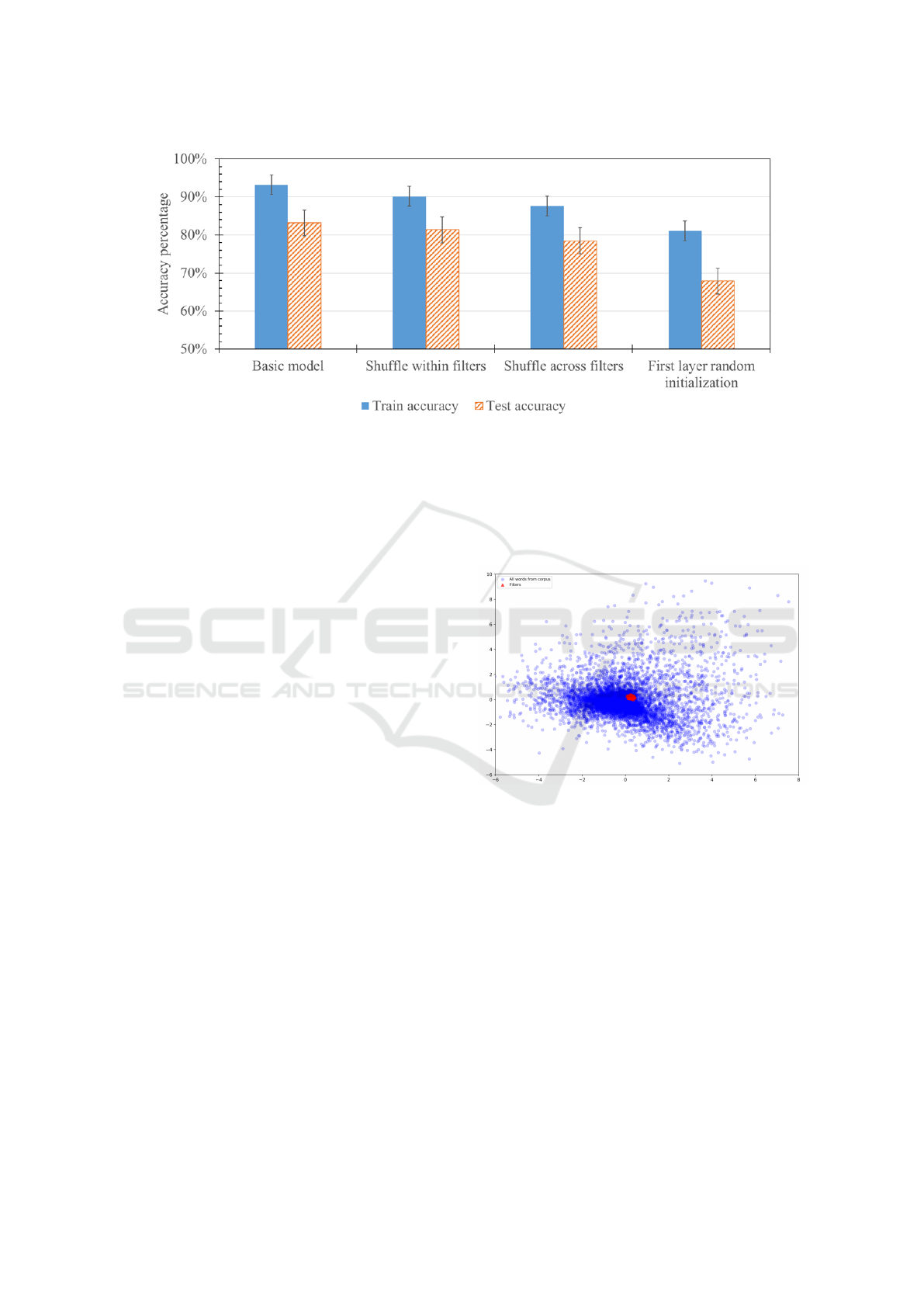
Figure 1: Comparison of models with shufﬂed ﬁlters.

shows that, when the ﬁrst layer is assigned randomly

and then frozen, accuracy is around 68%, 18% higher

than random prediction (as our target variable is bi-

nary and balanced). Even when the ﬁrst layer does not

learn anything or contribute to the classiﬁcation out-

comes, the rest of the model learns enough for modest

success.

When we train the ﬁrst layer normally (in the ba-

sic model), it contributes around 15% to overall per-

formance. 2/3 of this contribution belongs to the ﬁlter

value choices and 1/3 belongs to the order of the se-

quence in our ﬁlters. That is the reason that when

we shufﬂe all 160 (32 ﬁlters × 5 units in each ﬁlter)

weights across all ﬁlters, only around 5% of overall

accuracy is lost.

Based on these experimental results, we learned

that the ordering of each ﬁlter is much less impor-

tant, compared to the crucial ﬁlter values found by

a model. In addition, we also learned that the rela-

tionship between neighboring ﬁlter values is not es-

pecially strong, since not much performance is lost if

the positions of each value are randomized throughout

the convolutional layer.

4.2 Clustering on Words and Filters

Clustering is an efﬁcient way to understand patterns

within data. To investigate such patterns, we concate-

nated all of our word embeddings (23,363 × 100) and

our ﬁlters (160 × 100) to create k clusters. We tested

different k between 2 to 2000. The result of the clus-

tering can be seen in Table 3. No matter which size

k we choose, there is a single crowded cluster that

contains most of the words (e.g., when we produce

ﬁve clusters, 85 percent of words belong to one clus-

ter). The most crowded cluster contains all 160 ﬁlter

values. This means that in word embedding space,

most of the words are concentrated in a small part of

space, and our model chose our ﬁlters to be in that

space as well. Figure 2 shows how tightly the ﬁlter

values are concentrated in the main cluster of words

(using PCA to represent 100-dimensional embedding

vectors in two dimensions).

Figure 2: Words vs ﬁlters.

4.3 Performance of Models on Most

Important Words

After ﬁnding the importance rating of every single

word in our corpus according to Equation 1 , we cre-

ated six new models. All of them share the same ar-

chitecture as our basic model shown in Table 1, and

each of them is trained only on a subset of the corpus

of words. We choose the top n most important words

in our corpus and drop the rest. We train our brand

new models on these subsets of words from scratch

(weights randomly initiated). Even after dropping

95% of words and training a new model just on 5%

of the most important, the performance does not de-

crease signiﬁcantly. The performance of these models

is presented in Table 4.

ICPRAM 2021 - 10th International Conference on Pattern Recognition Applications and Methods

200

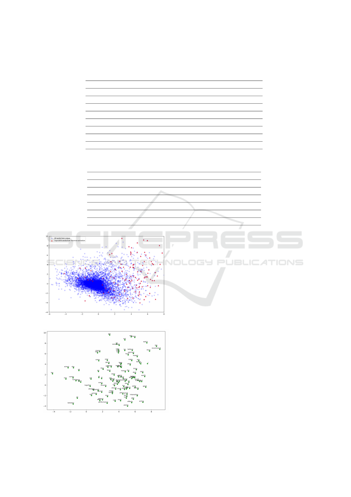
Table 3: Clustering results.

Sum of squared

distances

Count of elements in

most populated cluster

Percent of elements in

most populated cluster

1 - 23363 100.00

5 218924 19869 85.04

10 204173 14507 62.09

20 191238 11871 50.81

100 155071 8433 36.09

200 134379 7472 31.98

500 98158 5210 22.30

1000 63640 4936 21.13

2000 32948 2486 10.64

Table 4: New models trained on subset of words.

Words kept percentage Word counts Train accuracy Test accuracy

100.0 (Base Model) 23,363 93.24 83.19

80.0 18,691 92.71 83.16

50.0 11,682 93.43 83.14

10.0 2,337 92.83 83.67

5.0 1,169 92.34 82.53

1.0 234 87.02 78.16

0.5 117 84.75 74.62

Figure 3: Most important words vs all words.

Figure 4: Most important words.

Although the model does start to lose information,

and thus classiﬁcation performance, once the corpus

is reduced to 1% of its original size or below, perfor-

mance remains strong when using only 5% of avail-

able words. Our ﬁnal set of experiments focus on this

behavior. In ﬁgures 3 and 4, we used PCA to reduce

the dimensionality of the word embeddings from 100

to 2 in order to represent words in 2-D space, and

show how the most important words form a reason-

able coverage of the space. Figure 3 shows the im-

portant words as a fraction of all of the words, and

ﬁgure 4 shows which words were found to represent

the embedding space. The ﬁgures are separated for

clarity. To compare, we established three baseline

models: one which uses all words in our corpus, one

that also uses 5%, but selected randomly rather than

via Equation 1, and one that uses all except the most

important 5% of words. Results are shown in Table

5. Our selected words perform much better than ran-

domly choosing the 5% of words (a 20% increase in

test accuracy).

Table 5 and Figure 5 also show that restricting the

model to the most important words results in much

faster performance than the model using every avail-

able word in the corpus. Whether measured in epochs

or seconds, the restricted model is more than twice as

fast at learning. Unsurprisingly, speed is equivalent

between both models which use only 5% of the data,

Interpreting Convolutional Networks Trained on Textual Data

201

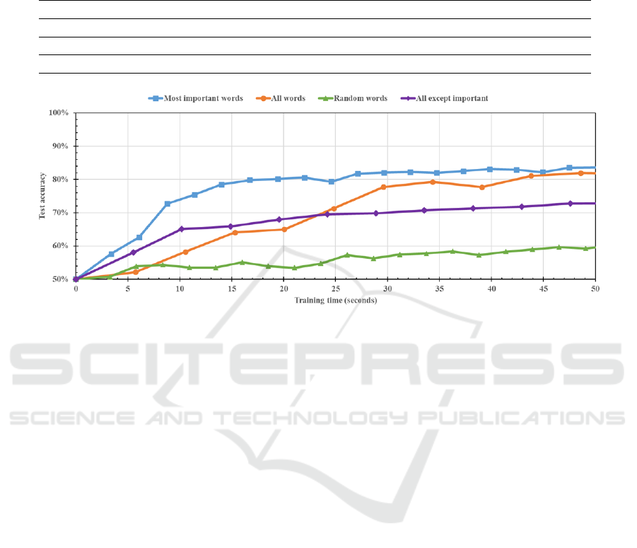
Table 5: Comparing new models to baseline models.

Model name

% words

used

Word

count

Train

accuracy

Test

accuracy

Average epoch

training time

(seconds)

Number of

parameters

Most important words 5% 1,169 93.67% 84.42% 36.3062 256,697

All words 100% 23,363 96.87% 85.33% 81.6395 2,476,097

Random words 5% 1,169 70.68% 64.29% 36.1543 256,697

All except important 95% 22,194 83.86% 74.52% 79.6917 2,359,197

Figure 5: Comparing our model with three baseline models based on testing accuracy and training time - points in each line

represent 1/20th of an epoch.

but one that uses the important words performs much

better. If the best 5% of words identiﬁed via Equa-

tion 1 are eliminated, the model has the worst of both

worlds and is neither fast nor accurate. The model

architecture and hyper-parameters seems to have in-

signiﬁcant effect on importance rate of words, but it

can be studied in more depth in future works.

5 CONCLUSION AND FUTURE

WORKS

The ﬁeld of machine learning has long focused on

how to improve the performance of our models, iden-

tify useful cost functions to optimize, and thereby

increase prediction accuracy. However, now that

human-level performance has been reached or ex-

ceeded in many domains using deep learning mod-

els, we must investigate other important aspects of

our models, such as explainability and interpretabil-

ity. We would like to be able to trust artiﬁcial intelli-

gence and rely on it even in critical situations. Fur-

thermore, beyond increasing our trust in a model’s

decision-making, a model’s interpretability helps us

to understand its reasoning, and it can help us to ﬁnd

its weaknesses and strengths. We can learn from the

model’s strengths and inject them into new models,

and we can overcome their weak points by removing

their bias.

In this paper, we investigated the logic behind the

decisions of a 1-D CNN model by studying and ana-

lyzing its ﬁlter values and determining the relative im-

portance of the unique words within a corpus dictio-

nary. We were able to use the insights from this inves-

tigation to identify a small subset of important words,

improving the learning performance of the training

process by better than double. Future work includes

expanding these techniques to investigate structures

beyond the ﬁrst layer of the convolutional network.

In addition, we are planning to deepen our study of

the ability of our model to identify important words.

By performing sensitivity analysis, alternately verify-

ing or denying the model’s access to words it deems

vital, we will hopefully be able to facilitate the trans-

fer of linguistic insights between human experts and

learning systems.

REFERENCES

Adadi, A. and Berrada, M. (2018). Peeking inside the black-

box: A survey on explainable artiﬁcial intelligence

(xai). IEEE Access, 6:52138–52160.

Arras, L., Horn, F., Montavon, G., M

uller, K.-R., and

Samek, W. (2017). ” what is relevant in a text docu-

ICPRAM 2021 - 10th International Conference on Pattern Recognition Applications and Methods

202

ment?”: An interpretable machine learning approach.

PloS one, 12(8).

Bach, S., Binder, A., Montavon, G., Klauschen, F., M

uller,

K.-R., and Samek, W. (2015). On pixel-wise explana-

tions for non-linear classiﬁer decisions by layer-wise

relevance propagation. PloS one, 10(7).

Bird, S., Klein, E., and Loper, E. (2009). Natural language

processing with Python: analyzing text with the natu-

ral language toolkit. ” O’Reilly Media, Inc.”.

Choi, K., Fazekas, G., and Sandler, M. (2016). Explaining

deep convolutional neural networks on music classiﬁ-

cation. arXiv preprint arXiv:1607.02444.

Collobert, R., Weston, J., Bottou, L., Karlen, M.,

Kavukcuoglu, K., and Kuksa, P. (2011). Natural lan-

guage processing (almost) from scratch. Journal of

machine learning research, 12(Aug):2493–2537.

Du, M., Liu, N., and Hu, X. (2019). Techniques for in-

terpretable machine learning. Communications of the

ACM, 63(1):68–77.

Gunning, D. (2017). Explainable artiﬁcial intelligence

(xai). Defense Advanced Research Projects Agency

(DARPA), nd Web, 2.

Hochreiter, S. and Schmidhuber, J. (1997). Long short-term

memory. Neural computation, 9(8):1735–1780.

Kalchbrenner, N., Grefenstette, E., and Blunsom, P. (2014).

A convolutional neural network for modelling sen-

tences. arXiv preprint arXiv:1404.2188.

Kim, Y. (2014). Convolutional neural networks for sentence

classiﬁcation. arXiv preprint arXiv:1408.5882.

Le, H. T., Cerisara, C., and Denis, A. (2018). Do convolu-

tional networks need to be deep for text classiﬁcation?

In Workshops at the Thirty-Second AAAI Conference

on Artiﬁcial Intelligence.

Li, J., Chen, X., Hovy, E., and Jurafsky, D. (2015). Visual-

izing and understanding neural models in nlp. arXiv

preprint arXiv:1506.01066.

Maas, A. L., Daly, R. E., Pham, P. T., Huang, D., Ng, A. Y.,

and Potts, C. (2011). Learning word vectors for sen-

timent analysis. In Proceedings of the 49th annual

meeting of the association for computational linguis-

tics: Human language technologies-volume 1, pages

142–150. Association for Computational Linguistics.

Mikolov, T., Sutskever, I., Chen, K., Corrado, G. S., and

Dean, J. (2013). Distributed representations of words

and phrases and their compositionality. In Advances in

neural information processing systems, pages 3111–

3119.

Montavon, G., Samek, W., and M

uller, K.-R. (2018). Meth-

ods for interpreting and understanding deep neural

networks. Digital Signal Processing, 73:1–15.

Pennington, J., Socher, R., and Manning, C. D. (2014).

Glove: Global vectors for word representation. In

Proceedings of the 2014 conference on empirical

methods in natural language processing (EMNLP),

pages 1532–1543.

Qin, Z., Yu, F., Liu, C., and Chen, X. (2018). How con-

volutional neural network see the world-a survey of

convolutional neural network visualization methods.

arXiv preprint arXiv:1804.11191.

Rajwadi, M., Glackin, C., Wall, J., Chollet, G., and Can-

nings, N. (2019). Explaining sentiment classiﬁcation.

Interspeech 2019, pages 56–60.

Rehurek, R. and Sojka, P. (2010). Software framework for

topic modelling with large corpora. In In Proceedings

of the LREC 2010 Workshop on New Challenges for

NLP Frameworks. Citeseer.

Ribeiro, M. T., Singh, S., and Guestrin, C. (2016). ” why

should i trust you?” explaining the predictions of any

classiﬁer. In Proceedings of the 22nd ACM SIGKDD

international conference on knowledge discovery and

data mining, pages 1135–1144.

Simonyan, K., Vedaldi, A., and Zisserman, A. (2013).

Deep inside convolutional networks: Visualising im-

age classiﬁcation models and saliency maps. arXiv

preprint arXiv:1312.6034.

Wang, F., Jiang, M., Qian, C., Yang, S., Li, C., Zhang, H.,

Wang, X., and Tang, X. (2017). Residual attention

network for image classiﬁcation. In Proceedings of

the IEEE Conference on Computer Vision and Pattern

Recognition, pages 3156–3164.

Wood-Doughty, Z., Andrews, N., and Dredze, M. (2018).

Convolutions are all you need (for classifying charac-

ter sequences). In Proceedings of the 2018 EMNLP

Workshop W-NUT: The 4th Workshop on Noisy User-

generated Text, pages 208–213.

Xu, K., Ba, J., Kiros, R., Cho, K., Courville, A., Salakhudi-

nov, R., Zemel, R., and Bengio, Y. (2015). Show, at-

tend and tell: Neural image caption generation with

visual attention. In International conference on ma-

chine learning, pages 2048–2057.

Yin, W., Kann, K., Yu, M., and Sch

utze, H. (2017). Com-

parative study of cnn and rnn for natural language pro-

cessing. arXiv preprint arXiv:1702.01923.

Yosinski, J., Clune, J., Nguyen, A., Fuchs, T., and Lipson,

H. (2015). Understanding neural networks through

deep visualization. arXiv preprint arXiv:1506.06579.

Zeiler, M. D. and Fergus, R. (2014). Visualizing and under-

standing convolutional networks. In European confer-

ence on computer vision, pages 818–833. Springer.

Interpreting Convolutional Networks Trained on Textual Data

203