PLEADES: Population Level Observation of Smartphone Sensed

Symptoms for In-the-wild Data using Clustering

Hamid Mansoor

, Walter Gerych

, Abdulaziz Alajaji

, Luke Buquicchio

, Kavin Chandrasekaran

Emmanuel Agu

1,2

and Elke Rundensteiner

1,2

Department of Data Science, Worcester Polytechnic Institute, Worcester, Massachusetts, U.S.A.

Department of Computer Science, Worcester Polytechnic Institute, Worcester, Massachusetts, U.S.A.

Keywords:

Interactive Visual Analytics, Smartphone Sensed Health, In-the-wild Smartphone Data.

Abstract:

Smartphones are increasingly being used for health monitoring. Training of machine learning health models

require studies in which smartphone sensor data is gathered passively on subjects’ phones. Subjects live their

lives ’In-the-wild” and periodically annotate data with ground truth health labels. While computational ap-

proaches such as machine learning produce accurate results, they lack explanations about the complex factors

behind the manifestation of health-related symptoms. Additionally, population-level insights are desirable

for scalability. We propose Population Level Exploration and Analysis of smartphone DEtected Symptoms

(PLEADES), a framework to present smartphone sensed data in linked panes using intuitive data visualiza-

tions. PLEADES utilizes clustering and dimension reduction techniques for discovery of groupings of similar

days based on smartphone sensor values, across users for population level analyses. PLEADES allows analysts

to apply different clustering and projection algorithms to a given dataset and then overlays human-provided

contextual and symptom information gathered during data collection studies, which empower the analyst in

interpreting ﬁndings. Such overlays enable analysts to contextualize the symptoms that manifest in smart-

phone sensor data. We visualize two real world smartphone-sensed datasets using PLEADES and validate it

in an evaluation study with data visualization and human context recognition experts.

1 INTRODUCTION

Health assessments are currently schedule-driven and

often infrequent. Smartphones provide a useful way

to monitor their users’ health status. They are ubiqui-

tous and come equipped with several sensors. Data

from those sensors have been used to infer health

markers such as Circadian Rhythms (sleep-wake cy-

cles) (Abdullah et al., 2017), depression (Gerych

et al., 2019; Saeb et al., 2015) and infectious diseases

(Madan et al., 2011). To create computational mod-

els that analyze user sensor data to make health in-

ferences, researchers need to conduct studies to col-

lect labeled datasets. In such studies, smartphone

sensed-data is passively gathered by an app on sub-

jects’ smartphones as they live their lives “in-the-

wild”. Periodically, subjects provide ground truth la-

bels on their health status by responding to health

and other contextual questions. Such health labels are

used to create supervised deep/machine learning clas-

siﬁcation models for future assessment of subjects.

Such an approach yields realistic but imperfect

data with missing ground truth labels and missing pe-

riods of data collection (Restuccia et al., 2017). The

streams of multi-variate data from multiple smart-

phone sensors are difﬁcult to understand without pre-

processing. Due to these issues, the factors that

caused user-reported symptoms may not always be

clear. It may be useful to have some way of group-

ing similar objective smartphone sensor data together

and overlaying human provided symptom and context

information to create linkages between them that may

increase explainability. For instance, linking reports

of disruptions in circadian rhythms (sleep-wake cy-

cles) with late night time smartphone screen usage

patterns which have been shown to accurately detect

sleep and waking times (Abdullah et al., 2017).

For large populations of smartphone-sensed health

subjects (Vaizman et al., 2018; Wang et al., 2014),

data science analysts may ﬁnd visualizations that link

human-reported symptoms to objective smartphone-

sensor data useful. For instance, visually linking

changes in user-reported sleep duration and quality to

Mansoor, H., Gerych, W., Alajaji, A., Buquicchio, L., Chandrasekaran, K., Agu, E. and Rundensteiner, E.

PLEADES: Population Level Observation of Smartphone Sensed Symptoms for In-the-wild Data using Clustering.

DOI: 10.5220/0010204300640075

In Proceedings of the 16th International Joint Conference on Computer Vision, Imaging and Computer Graphics Theory and Applications (VISIGRAPP 2021) - Volume 3: IVAPP, pages 64-75

ISBN: 978-989-758-488-6

their smartphone-sensed sleep location (e.g. primary

residence [normal] vs. workplace [abnormal]) may

contextualize and explain their sleep patterns. Visual-

izations over longer periods may also be useful in sep-

arating one-off behaviors from patterns. For instance

visualizing disruptions in sleep along with mobility

patterns over long periods of time may help distin-

guish mentally healthy subjects who travel more and

thus have occasional sleep disruptions from mentally

ill people who primarily stay at one place and still

report sleep disruptions (Mendes et al., 2012). This

enables analysts to ﬁlter, select and label participants

with days that have potentially concerning symptoms

to generate classiﬁcation models that can then be used

to assess other current or future participants.

Unsupervised clustering facilitates scalable visu-

alization and sense-making of large, multi-variate,

data by grouping similar data points (Cavallo and

Demiralp, 2018; Kwon et al., 2017). As the re-

sults of clustering algorithms are still in a high di-

mensional space, they can then be projected to be

more easily visualizable on two dimensional planes

using dimension reduction techniques. Examples in-

clude t-Distributed Stochastic Neighbor Embedding

(t-SNE) (Maaten and Hinton, 2008), Isomap (Tenen-

baum et al., 2000) and Multi-dimensional Scaling

(Mead, 1992), which can work with a large number

of data points and features. Clustering and project-

ing using dimension reduction is often an exploratory

process which can become overwhelming given the

large number of clustering and projection algorithms

(Cavallo and Demiralp, 2018; Kwon et al., 2017). It is

also important to keep track of the smartphone-sensed

features and human applied symptom and context la-

bels across different clustering results to assign asso-

ciations between them. For example, a cluster of days

with lower reported sleep quality may be explained

by higher night time smartphone usage. In addition,

there also needs to be some method of assessing the

role of each data feature with regards to the clustering

result to understand the differences between clusters.

We present Population Level Exploration and

Analysis of smartphone DEtected Symptoms

(PLEADES), a visualization framework that displays

smartphone-sensed data using multiple linked panes.

PLEADES enables analysts to ﬂexibly select clus-

tering and projection algorithms, as well as features

which are used for clustering. It then computes the

clusters for all the study days across all selected

participants and presents the clustering results as hor-

izontally stacked bars, with the colors representing

the cluster and the width of each bar representing

the proportion of days in that cluster. The cluster-

ing results are then ordered by clustering quality

metrics such as silhouette score (Rousseeuw, 1987),

Davies-Bouldin score (Davies and Bouldin, 1979)

and Calinski-Harabasz score (Cali

nski and Harabasz,

1974). Being able to select only features relevant

to a given task may enable analysts to focus and

observe important patterns in speciﬁc categories of

smartphone-sensed behavior (e.g. mobility), reducing

the confounding effects of irrelevant features.

PLEADES also supports ﬁltering study partic-

ipants, allowing analysts to compare the results

of multiple techniques across different populations,

providing more intuition than traditional non-visual

methods of exploratory data analysis. This en-

ables comparisons between sub-populations of partic-

ipants with very different smartphone sensor data for

clearer understanding of the semantic factors leading

up to differences that manifested themselves in the

smartphone-sensed data. For instance, frequent trav-

ellers will have different location signals than stay-

at-home people, and clustering days based on those

location features may allow analysts to identify these

groups and contextualize reported symptom data.

Speciﬁcally our contributions include:

• PLEADES, an interactive visualization tool that

facilitates ﬂexible and reproducible population-

level exploratory data analysis of smartphone-

sensed symptom data using multiple clustering

and dimension reduction techniques and visualiz-

ing their results in multiple linked panes.

• Insightful walk-throughs of illustrative use cases

that demonstrate the utility of PLEADES to fos-

ter clearer understanding of in-the-wild collected

health related smartphone data.

• Evaluation of PLEADES with experts in smart-

phone sensed health and data visualizations.

2 RELATED WORK

2.1 Analyzing Smartphone Data

Smartphone sensed data has clues about user be-

haviors and health symptoms such as coughing and

sneezing caused by inﬂuenza (Madan et al., 2011)

and abnormal mobility patterns caused by mental ill-

ness (Mohr et al., 2017). Smartphone sensed data has

semantically important information and can be pre-

dictive of health. For instance, GPS trajectories have

been used to predict depression (Gerych et al., 2019;

Saeb et al., 2015; Canzian and Musolesi, 2015). Ab-

dullah et al. (Abdullah et al., 2017) used screen in-

teractions at night to detect disruptions in Circadian

Rhythms (sleep-wake patterns), which have health

PLEADES: Population Level Observation of Smartphone Sensed Symptoms for In-the-wild Data using Clustering

ramiﬁcations (Vetter, 2018). In StudentLife, Wang et

al. (Wang et al., 2014) used objective smartphone-

sensed data to assess students’ mental health and

their academic performance. Wang et al. (Wang

et al., 2020) collected social functioning measures and

smartphone sensor data, which they used to predict

the social functioning of patients with schizophrenia.

Much of the smartphone sensing research above

has focused on using machine learning to build pre-

dictive models. However, such approaches provide

limited explanations. Data visualizations can rep-

resent highly multivariate and complex smartphone

sensed data. Shen and Ma created MobiVis (Shen and

Ma, 2008), an interactive visualization tool that rep-

resented individual and group behaviors compactly

using the “Behavior Ring”, a radial metaphor. Mo-

biVis enabled visual data mining by semantic ﬁltering

for analysis of “social-spacial-temporal” phone data.

Senaratne et al (Senaratne et al., 2017) used interac-

tive visualizations to analyze spatio-temporal similar-

ities in human movements using phone data. They

used matrix visualizations of the user movements. Pu

et al. (Pu et al., 2011) utilized voronoi-based maps

and parallel coordinates plots to visualize mobility

patterns across a large number of users.

These works show the usefulness of interactive

data visualizations to understand human movement

(an important facet of life), its variations and disrup-

tions. Our work adds to this ﬁeld by using multiple

linked panes to overlay human reported symptom data

on objective sensor data to guide intuition during ex-

ploratory data analysis, to inform the building of ma-

chine learning classiﬁers. Moreover, our work visual-

izes not only mobility data but a more comprehensive

set of smartphone-sensed features including user ac-

tivity levels and screen interaction patterns.

2.2 Clustering Multivariate Data

Unsupervised clustering is a useful technique for

grouping similar data, facilitating exploratory anal-

ysis of large datasets. Clustering results are in a

high dimensional space and can be visualized after

using dimension reduction to project them onto a

2D plane. Such projection enhances interpretability

(Sacha et al., 2016). Analysts can use domain knowl-

edge to perform interactive tasks such as merging

and assigning data points to speciﬁc clusters for ﬂex-

ible understanding (Wenskovitch and North, 2019;

Boudjeloud-Assala et al., 2016) as no computational

model can ﬁnd a perfect solution that separates data

into meaningful clusters and account for all the com-

plexities in multi-feature data. Researchers have used

these techniques for data in domains such as social

media (Hoque and Carenini, 2015), bio-informatics

(L’Yi et al., 2015) and crimes (Fujiwara et al., 2019),

demonstrating their diverse applicability.

Tracking multiple iterations of clustering and

dimension reduction techniques can become over-

whelming. Kwon et al. (Kwon et al., 2017) cre-

ated Clustervision, an interactive visualization tool to

present ranked results across multiple dimension re-

duction and clustering algorithms for ﬂexible anal-

ysis of multi-dimensional data. They projected the

clusters on a 2-D view, linked with contextual vi-

sualizations such as a parallel coordinates plot and

bar charts with information about the selectable data

points. Cavallo et al. (Cavallo and Demiralp, 2018)

created Clustrophile 2, a visual tool to perform Ex-

ploratory Data Analysis by tuning dimension reduc-

tion parameters and features. They introduce the

”Clustering Tour”, for exploratory data analysis, by

presenting data using visualizations like feature aver-

age heatmaps. Chatzimparmpas et al. (Chatzimparm-

pas et al., 2020) created t-viSNE, a visual analytics

tool to let users analyze the results of t-SNE for better

understandability of the results using multiple linked

panes with bar charts and parallel coordinate plots.

Our contribution is utilizing visual clustering and

projection techniques to a new domain namely com-

plex smartphone sensed data. For explanability, we

overlay human-supplied labels along with computed

semantic information such as presence of weekdays

and weekends over objective smartphone sensor data

to enable analysts to discover important relationships

in the data during early exploratory data analysis.

3 GOAL AND TASK ANALYSIS

We conducted a goal and task analysis with four

experts in generating machine learning models for

health predictions using smartphone-sensed data. The

experts wanted interactive analysis for early stage ex-

ploration before training and testing machine learn-

ing models. Interactive clustering and projection is a

powerful method for exploratory data analysis (Cav-

allo and Demiralp, 2018; Kwon et al., 2017; Chatzim-

parmpas et al., 2020). The experts wanted Population

Level information of study cohorts for scalability as

the size and scope of such studies increase. From this

view, they wanted the ability to drill down on speciﬁc

study participants. In this population-level view of the

data, they were interested in: 1) Viewing clustering

results and groupings of objective sensor data such as

clusters of days with higher mobility vs. clusters of

days with lower mobility etc. and 2) linking any cor-

responding human-provided context and symptom la-

IVAPP 2021 - 12th International Conference on Information Visualization Theory and Applications

bels such as clusters of days with higher mobility also

having poorer overall sleep etc., that may help them

assign semantic information to the objective sensor

data. The analysts also suggested using a window of

24 hours (one day) to divide up the data per user as

human behaviors are strongly inﬂuenced by daily cy-

cles (Vetter, 2018). We summarize a list of goals that

the experts would have while analyzing such data and

the tasks to accomplish them:

Goal 1. Grouping similar participant days. Clearly

view groupings of days across multiple participants

that are similar in terms of objective sensor data such

as clusters with higher activity levels vs. sedentary

clusters etc.

• Task 1: Giving analysts the ability to select and

ﬁlter features for smartphone sensor data to be

considered for clustering, to analyze speciﬁc be-

haviors (e.g. smartphone-detected activity levels

or mobility patterns).

• Task 2: Applying clustering and then dimension

reduction techniques to effectively display similar

days on a two-dimensional plane. Different clus-

ters will be color-coded.

• Task 3: Display the results of multiple iterations

of projection and clustering algorithms for ﬂexi-

ble analyst interpretation. To ensure validity, re-

sults will be ordered using standard clustering re-

sult quality metrics such as silhouette scores etc.

Goal 2. Understand the causative factors behind the

clustering results.

• Task 4: Show smartphone-sensed features that are

most important for each clustering result. This

will inform analysts about the factors that are most

important for cluster separation. For example, a

clustering result might assign screen interaction

levels across different epochs more importance

and the clusters may be separated by high screen

interaction vs. low screen interaction.

• Task 5: Show the variation of feature values be-

tween different clusters to enable analysts to as-

sign semantic meaning to them. For example clus-

ters with higher levels of being present at home vs.

not being at home etc.

Goal 3. Compare individuals to populations along

with sub-populations to other sub-populations to ﬁnd

interesting clusters and groupings of users.

• Task 6: Show a list of all the users with the ability

to select and ﬁlter a sub-set for clustering analysis.

• Task 7: Show the distribution of clusters for each

individual’s data for semantic meaning assign-

ment. For instance, showing if an individual has

more days in a cluster with higher mobility etc.

Goal 4. Overlay human labelled information on ob-

jective smartphone sensed data to allow analysts to

assign semantic meaning to data like clusters with

days having higher night time screen usage also hav-

ing poorer reported sleep and higher stress levels etc.

• Task 8: Present summaries of human-labelled

symptom data such as overall sleep quality, stress

etc. for every cluster, along with the ability to ﬁl-

ter and select speciﬁc days for analysis.

• Task 9: Show external day-level factors that may

explain the symptoms present (e.g. weekend vs

weekdays, academic deadlines etc.)

Goal 5. Saving exploration results.

• Task 10: Storing results from an analysis session

to share with other analysts to save time as clus-

tering is computationally intensive.

4 OUR VISUAL APPROACH:

PLEADES

We present Population Level Exploration and Analy-

sis of smartphone DEtected Symptoms (PLEADES),

an interactive visual analytics framework that uses

multiple linked views to present smartphone sensed

data. We divided all participant data into individual

days and calculated day level features for sensor val-

ues across multiple epochs such as day, evening and

night. The analyst can start by selecting a dataset

(ReadiSens or StudentLife (Wang et al., 2014)) along

with features for the data to be clustered on (G1, T1)

and the participants (by default all participants are in-

cluded).

Here we describe the main views and the rationale

behind the design.

4.1 Algorithms Selection and Features

View

The analyst can select from three dimension reduction

(t-SNE, Isomap and multi-dimensional scaling) and

three clustering (kMeans, agglomerative and spectral)

techniques in (Figure 1 H). Clicking on the “Features

View” (FV) shows the dialog (Figure 1 I) to present

all the sensor values along with the epochs that those

sensor values should be averaged by, to be consid-

ered as features that can be input into the clustering

and projection algorithms (G1, T1). Through exten-

sive user studies, Cavallo and Demiralp (Cavallo and

Demiralp, 2018) reported that analysts spent consid-

erable effort on feature selection during exploratory

data analysis using clustering and projection methods

as it was very important for the outcomes.

PLEADES: Population Level Observation of Smartphone Sensed Symptoms for In-the-wild Data using Clustering

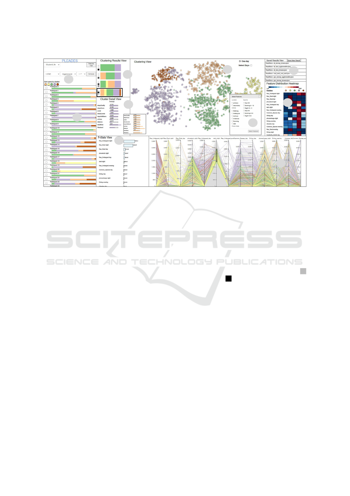
Figure 1: PLEADES: A) Every multi-colored bar represents a clustering result for the algorithms and k chosen, ordered by

their “quality”, calculated across several state of the art methods. The width of each colored bar in the multi-colored bars

represents the proportion of days in that cluster. B) Selecting a result projects it on a 2-D plane with every circle representing

one day, color coded to the cluster it belongs to. C) Hovering over any day in the Clusters View shows that day’s cluster’s

details in the Cluster Detail View. Details include average reported sleep quality for the cluster vs. the overall etc. D)

Every study participant is a row in the Users View and the colored bars represent distribution across the clusters for their

days in study. E) The distribution of feature value intensity across all clusters is shown in the Feature Distribution Heatmap.

F) The F-Stats View shows a bar chart for the most important features for the selected clustering result, determined by the

ANOVA F-Statistic. G) Every polyline is a day with the color representing the cluster. The axes represent features and are

brushable i.e analysts can select ranges of values. H) Analysts can select the clustering and dimension reduction algorithms.

I) Selecting features and their epochs for averaging. These features will be calculated for all days which will then be clustered.

J) Pre-computed clustering results from previous sessions are displayed to save analysts’ time.

4.2 Clustering Results View

Clustering creates groups of days that are similar

based on a set of selected features and metrics.

The Clustering Results View (CRV) displays mul-

tiple clustering results as horizontally stacked bars

with the colors representing the cluster and the width

representing the proportion of total days that belong

to that cluster (Figure 1 A). The results are ordered

by quality (G1, T2, T3). Using multiple cluster-

ing and projection algorithms enables ﬂexible explo-

ration of various aspects of the data for more intu-

ition. This approach was inspired by Kwon et al.

who implemented Clustervision (Kwon et al., 2017)

and displayed multiple clustering results ordered by

quality for speciﬁed clustering and projection algo-

rithms. The results are ordered by the highest aver-

age across three clustering quality measures: Silhou-

ette score (Rousseeuw, 1987), Davies-Bouldin score

(Davies and Bouldin, 1979) and Calinski-Harabasz

score (Cali

nski and Harabasz, 1974) (G1, T3). The

scores are represented in the mentioned order as small

squares to the left of the clustering results, with higher

opacity representing higher quality (low quality:

vs. high quality: ). We used ColorBrewer (Har-

rower and Brewer, 2003) to assign each cluster a dis-

cernible color using an 8 color palette (G1, T2).

4.3 Clusters View (CV)

The Clusters View (CV) presents the projection of the

selected clustering result in the CRV on a 2-D plane

where every point is a day and the color encoding the

cluster (Figure 1 B). This visually represents days that

are similar according to the clustering result (G1, T2).

Combined with the clustering results view, the analyst

can quickly and easily see the size of the various clus-

ters along with the overlaps between clusters.

If the analyst wants to drill down on speciﬁc days

for further analysis, they can check the “Select Days”

box and brush over the days they are interested in the

CV, which will subsequently show the aggregated de-

tails for the selected day in the Cluster Details View

and highlight them in the Daily Values View (ex-

plained later). The analyst can also save the days

and the associated users by giving the days a name

IVAPP 2021 - 12th International Conference on Information Visualization Theory and Applications

in the dialog that shows up after the days are brushed

(G5, T10). This allows analysts to use their domain

knowledge to determine whether certain days belong

in a cluster. This is also meant to assist analysts in

classifying the types of days that can be used for clas-

siﬁcation models and also to assign any meaningful

semantic information, such as low stress and better

sleep on days that are typically weekends.

4.4 Cluster Details View (CDV)

The Cluster Details View (CDV) (Figure 1 C) shows

aggregated details for all the days in a cluster being

hovered over in the CV, to be compared to the overall

average across all clusters (G4, T8, T9). The bar with

the grey stroke represents the overall

average across all days and participants. The color

of the ﬁll inside represents the cluster of the day that

is being hovered over in the CV. In case the analysts

has selected speciﬁc days in the CV, the ﬁll color is:

. The aggregated details include information such

as comparisons with the average occurrence of week-

ends in that cluster, the average amount of distance

travelled and average sleep quality reported.

4.5 Users View (UV)

The User’s View (UV) (Figure 1 D) shows a list of

the individual participants in the smartphone-sensed

symptoms studies. The colored bars in each partic-

ipant’s row represent the distribution of clusters for

every individual user’s days for the clustering result

selected (G3, T7). The analyst can sort the user list by

the prevalence of days in a speciﬁc cluster, by click-

ing on its respective color under “Sort users by clus-

ter” (G3, T6) (Figure 1 H). Hovering over a user’s row

shows their days highlighted in the Clusters View and

the Daily Values View (explained later) and hides oth-

ers’ days (G3, T7). The user can be selected for re-

clustering by clicking on their checkboxes (G3, T6).

4.6 F-Stats View (FSV)

The F-Stats View (FSV) (Figure 1 F) shows the most

important features for creating the clusters (those

that have a statistically signiﬁcant relationship) as a

ranked bar chart. This helps an analyst reason about

the proportion of importance of each feature and the

causes of separation between clusters (G2, T4). We

perform the Analysis Of Variance (ANOVA) test for

every clustering result to obtain the f-statistic, along

with its associated p-value across all clustering fea-

tures that measures the importance and statistical sig-

niﬁcance of each feature for the clustering result.

4.7 Feature Distribution Heatmap

(FDH)

The Feature Distribution Heatmap (FDH) (Figure 1

E) shows the average values of the selected features

across all the different clusters using a gradient of

dark blue to dark red to represent very low and very

high respectively (G2, T5). The features are ordered

from the top to bottom in terms of their importance

(shown in FSV). It is important to show the distribu-

tions of feature values across all the clusters to help

analysts understand characteristics of the days within

each cluster. This allows an analyst to quickly assign

semantic meaning to speciﬁc clusters.

4.8 Daily Values View (DVV)

Every day across all its features is plotted as a poly-

line in a parallel coordinates plot in the Daily Values

View (DVV) (Figure 1 G). The y-axes are brushable

for ﬁltering speciﬁc ranges of features values. The

lines are color-coded to the cluster they belong to.

This view lets analysts ﬁlter down on speciﬁc features

and assign semantic meaning to clusters (G4, T8).

4.9 Saved Results View (SRV)

SRV can save the results of exploration sessions.

Clustering multi-feature data is computationally in-

tense and re-running clustering every time is not scal-

able. In addition, analysts may want to share their

insights for reproducibility. We allow the user to save

the results from the clustering session they performed

by clicking on the “Save New Result” button in the

Saved Results View (SRV) (Figure 1 J) and providing

a name that can then be selected for viewing from the

list every time PLEADES is started (G5, T10).

5 EVALUATION WITH USE

CASES

We now introduce Luna, a graduate student specializ-

ing in computational social science and psychology.

Luna has access to two datasets and she would like

to perform exploratory data analysis on both of them

using PLEADES. Speciﬁcally, she is interested in

understanding relationships between symptoms and

objective sensor data. This information can guide

her creation of machine learning models that classify

smartphone user symptoms from sensed data.

PLEADES: Population Level Observation of Smartphone Sensed Symptoms for In-the-wild Data using Clustering

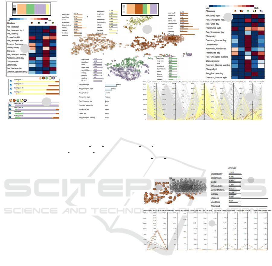
Figure 2: kMeans clustering of every day across every participant based on the similarity of their geo-location features. The

results are then projected using t-SNE. A) A clustering result with k=3 and high quality (Davies-Bouldin score) and the

associated Feature Distribution Heatmap. B) Selecting a result with k=5. Cluster details are shown for the ﬁve clusters. The

yellow cluster has high presence in “Res Grad night” and “Res Grad day”, whereas the green and purple clusters have high

values for presence in the “Res Undergrad day, evening and night”, possibly indicating two different student populations i.e.

graduate students and undergraduate students. E) Brushing over “Res

Grad night” shows no purple or green lines.

5.1 StudentLife (Dataset 1)

The ﬁrst dataset is StudentLife (Wang et al., 2014)

which has data for 49 Dartmouth University students

over a 10 week academic term. The students in-

stalled an application on their smartphones which pas-

sively and continuously gathered sensor data includ-

ing screen interaction, light levels, conversations, ac-

tivity levels (walk, run, still) and on-campus location,

using WiFi connection points for on campus build-

ings. The buildings are binned into categories such as

undergraduate-residential, graduate-residential, din-

ing, academic and administrative services. The ap-

plication also gathered GPS coordinates that we clus-

tered using DBSCAN (Ester et al., 1996). We only

used the primary and secondary location, deﬁned as

the geo-cluster where the students spent the most and

the second most time in. Students also responded

to daily questionnaires about their stress levels, sleep

quality, socializing issues and hours of sleep.

The data was divided into days for every partici-

pant and the features (selected by the analyst in the

FV) are calculated per day. All the days across all

participants are then clustered and projected using the

analyst-selected algorithms. Mobility statistics are

computed for every cluster in the clustering result

such as the average distance travelled and the average

location entropy i.e. how many different geo-clusters

they visit as these features have been linked to symp-

toms (Madan et al., 2011; Saeb et al., 2015; Gerych

Figure 3: Days in the selected clump seem to have very

little presence on campus. In addition, these days are far

more likely to be weekends then the average, along with

much higher than average distance being travelled.

et al., 2019). Additionally, we calculate the propor-

tion of weekends in every cluster and visualize them

against the overall average along with the proportion

of days in “midterm”, an academically demanding

time at Dartmouth. Wang et al. (Wang et al., 2014)

mentioned that data gathered for weekdays would dif-

fer from weekends along with days in midterms.

5.2 Use Case 1: Quick Overview

Luna would like an overview of the data. She selects

all the sensor values across 3 epochs (day, evening

and night) to be clustered and projected using ag-

IVAPP 2021 - 12th International Conference on Information Visualization Theory and Applications

A B

Figure 4: After clustering potential grad and undergrad

students, there are four clusters of undergraduate students.

This can help insights by observing how undergraduates

differ in their behaviors and how their smartphone labelled

symptoms manifest in objective sensor data.

glomerative clustering (for up to k = 6 clusters) and

t-SNE (G1, T1). She selects the clustering results

with three and four clusters (second and third high-

est quality) (G1, T3). Interacting with the clusters in

the CV reveals nothing interesting in the CDV. She se-

lects fourth the highest quality clustering result with

k = 5 (Figure 1 A), which has good quality (Davies-

Bouldin score) (G1, T3). She also notices in the F-

Stats View that on-campus building presence features

(Res Undergrad, Common Space, Dining) are impor-

tant features for this clustering (G2, T4). She hovers

over the clusters in the CV to see the overall values

associated with each cluster in the CDV. She notices

that days in cluster (Figure 1 B), tend to have more

deadlines, poorer sleep quality, higher stress levels

and generally tend to fall on weekdays (Figure 1 C)

(G4, T8, T9). This makes sense to Luna as deadlines

can induce behavioral changes. In contrast, the clus-

ter has more days on the weekends, fewer dead-

lines and slightly better sleep duration and quality,

and more distance travelled. Such clear contrasts en-

courages Luna to delve further into the analysis. She

saves this clustering session using the SRV and names

it “more deadlines, less sleep” (G5, T10).

5.3 Use Case 2: Determining Student

Characteristics to Utilize for

Insightful Comparisons

Looking at the FSV, Luna realizes that features for

smartphone detected presence in on campus resi-

dences were important. To analyze this further, she

selects only the location features (on campus build-

ings and primary and secondary geo-locations) (Fig-

ure 1 H) and re-clusters the data using K-Means (k

= 6) and t-SNE for all participants. She selects a

clustering with good quality and k = 4 (Figure 2 A).

She notices in the FDH that there are two clusters in

which the days had high presence in Res Undergrad

and one cluster with high presence in Res Grad. She

wants to see some more distribution of features and

selects a clustering result with k = 5 (Figure 2 B).

Cluster (Figure 2 B) has higher than average val-

ues of being in Res Undergrad at all times of day

(Figure 2 C) and cluster has much higher than av-

erage incidence of being in other on-campus build-

ings such as Dining, Libraries, Academic etc. (G2,

T5). Days in cluster have no incidence of being

in Res Undergrad and fewer than usual incidences of

being in other on-campus building, with the only ex-

ception being Res Graduate (Figure 2 C). Sorting the

UV (Figure 2 D) using all three clusters and brushing

on the “Res Grad night” axis (Figure 2 E) shows that

there are no users who have days in both cluster

and cluster (G3, T6).

This is an indication of two sub-populations (G3,

T7) to Luna as she is aware that the StudentLife

(Wang et al., 2014) study included both graduate and

undergraduate students. Luna believes that the users

with days in clusters and are undergraduate

students whereas the users with days present in

represent graduate students. This is important for her

as one of the goals she had for analysis was compar-

ing symptoms and behavior patterns between differ-

ent populations. Graduate and undergraduate students

typically differ in their ages along with courseloads

and other life circumstances. She looks at the de-

tails for the three clusters in the CDV and notices that

for cluster (Figure 2 B) students reported slightly

worse sleep and slightly more stress than usual along

with more deadlines (G4, T8). Interestingly, for clus-

ter (Figure 2 B), students reported fewer than av-

erage deadlines along with average sleep quality and

slightly lower stress levels. The students in cluster

do not report any particularly concerning symptoms

(Figure 2 B). She saves the results from this session

in the SRV and calls it “geo analysis” (G5, T10).

Overlaying levels of semantically understandable

information like the types of on-campus buildings

along with sorting users by clustering results made the

discovery of these two populations of students easier

for Luna. In addition, she notices in the FDV that for

the cluster , there appear to be few days of presence

in any on-campus building (Figure 2 C). She hovers

over a day in that cluster and notices the bars in the

CDV show that students travelled much more distance

(Figure 2 B) than usual for these days along with the

fact that there were many more days on the weekends,

which makes intuitive sense (G4, T9). Luna notices

a peculiar shape in (Figure 3 A) and selects those

days by clicking on “Select Days” (Figure 1 B) and

then brushing over it. She notices in the CDV (Figure

PLEADES: Population Level Observation of Smartphone Sensed Symptoms for In-the-wild Data using Clustering

3 B) that the days in this clump are much more likely

to be weekends than the overall cluster , along with

much higher distance being travelled. She also no-

tices in the DVV (Figure 3 C) that there is little to

no presence for all the days in on-campus buildings.

She is now conﬁdent that these days represent travel.

In addition, she notices slightly better sleep quality,

more hours of sleep and fewer deadlines. This is in-

teresting as Luna is now able to assign semantically

relevant context to objective sensor data. She also

plans to build classiﬁcation models using these days,

which can ﬁnd similar days in other clusters. She la-

bels these days “travelling off campus” (G5, T10).

5.4 Use Case 3: Clustering Graduate vs.

Undergraduate Students

Luna is now interested in analyzing the two distin-

guishable populations in comparison to each other.

She selects the students in the UV that she feels con-

ﬁdent are more likely to belong to either cohort (8

graduates and 15 undergraduates) and re-clusters their

data using the same algorithms and k = 6 (G3, T6,

T7). She selects a result with k = 6 and views the

FDH to gain similar intuition to the last use case

about the graduate and undergraduate students by

noticing the distribution of presence incidence of on-

campus buildings. She can see four clusters

where the participants had reported high in-

cidence of being in Res Undergrad and one cluster

with higher Res Graduate (Figure 4 C). Interact-

ing with shows higher than average days being in

the midterm with poorer than average sleep quality

(Figure 4 A), but interestingly less stress and socia-

bility issues (G4, T8). For the cluster , Luna no-

tices more than average distance travelled along with

slightly worse sleep and stress levels (Figure 4 B). She

now has a ﬁner grain view of a population she iden-

tiﬁed earlier. She clicks “Save New Result” to show

her analysis to her colleagues (G5, T10).

5.5 ReadiSens (Dataset 2)

The second dataset is called ReadiSens. It has data

for 76 participants in a large study with smartphone

sensed data and reported symptoms such as sleep du-

ration and quality. The participants were asked to

install the ReadiSens collection application that ran

passively in the background and solicited daily and

weekly symptom reports. The participants have been

completely anonymized. The sensors include GPS lo-

cations and phone measurements such as activity lev-

els, screen usage and sound levels. The geo-location

data is used to derive mobility features in the same

way as the previous dataset and is also clustered the

same way to derive participants’ primary and sec-

ondary locations. The participants were asked to pro-

vide answers about sleep duration and quality ev-

ery day through a smartphone administered question-

naire, with varying levels of compliance. We divided

up the sensor data per day across all users and calcu-

lated the same mobility and contextual features (e.g.

proportion of weekends) as the StudentLife dataset.

5.6 Use Case 4: Presence in Primary

Location vs. Secondary Location

Luna visualizes ReadiSens data using PLEADES. She

selects all the features across all epochs, Isomap and

kMeans and k = 6. She views some clustering results

in the CV and their details in CDV but cannot seem to

ﬁnd any cluster that stands out (G1, T2, T3). She de-

cides to drill down on a speciﬁc sensor type (G1, T1).

She selects primary and secondary geo-clusters (the

geo-clusters where the participant spent the most and

the second most amount of time respectively) across

the 3 epochs and clusters the data using Isomap and

kMeans (k = 6) for projection and clustering. Partici-

pants’ locations have important bearing on symptoms.

Location can be indicative of home (Gerych et al.,

2019) vs. work schedules which in turn have impor-

tant health ramiﬁcations (Ravesloot et al., 2016).

Luna selects a result with k = 6 and hovers over

some clusters (Figure 5 A) and notices that for days

in cluster , participants tended to stay in in their

primary location for all the 3 epochs. Luna sees that

these days were more likely to be weekends, with

less distance travelled and more than average sleep

reported (G4, T8, T9). Luna believes that the days

in represent times where a person stayed “home”.

She assigns this semantic information to this cluster.

Next she interacts with cluster and notices

these days are less likely to be weekends (Figure 5

A). In addition, participants tend to be in their sec-

ondary location more during the day and evening with

little presence in the secondary position at night (Fig-

ure 5 B). Participants also tended not to be at their

primary location during the day and are a little more

present there during evening. But they usually are

there for the night (Figure 5 B). Participants also trav-

elled more distance than usual and report fewer than

average sleep hours. This leads Luna to guess that

these days belong to a work vs. home routine and

she make a note for that by saving this clustering ses-

sion in the SRV. This is useful for her as this speciﬁc

behavior has long term health ramiﬁcations (Raves-

loot et al., 2016). In addition, since this is an ongoing

project, the classiﬁers she builds using data for those

IVAPP 2021 - 12th International Conference on Information Visualization Theory and Applications

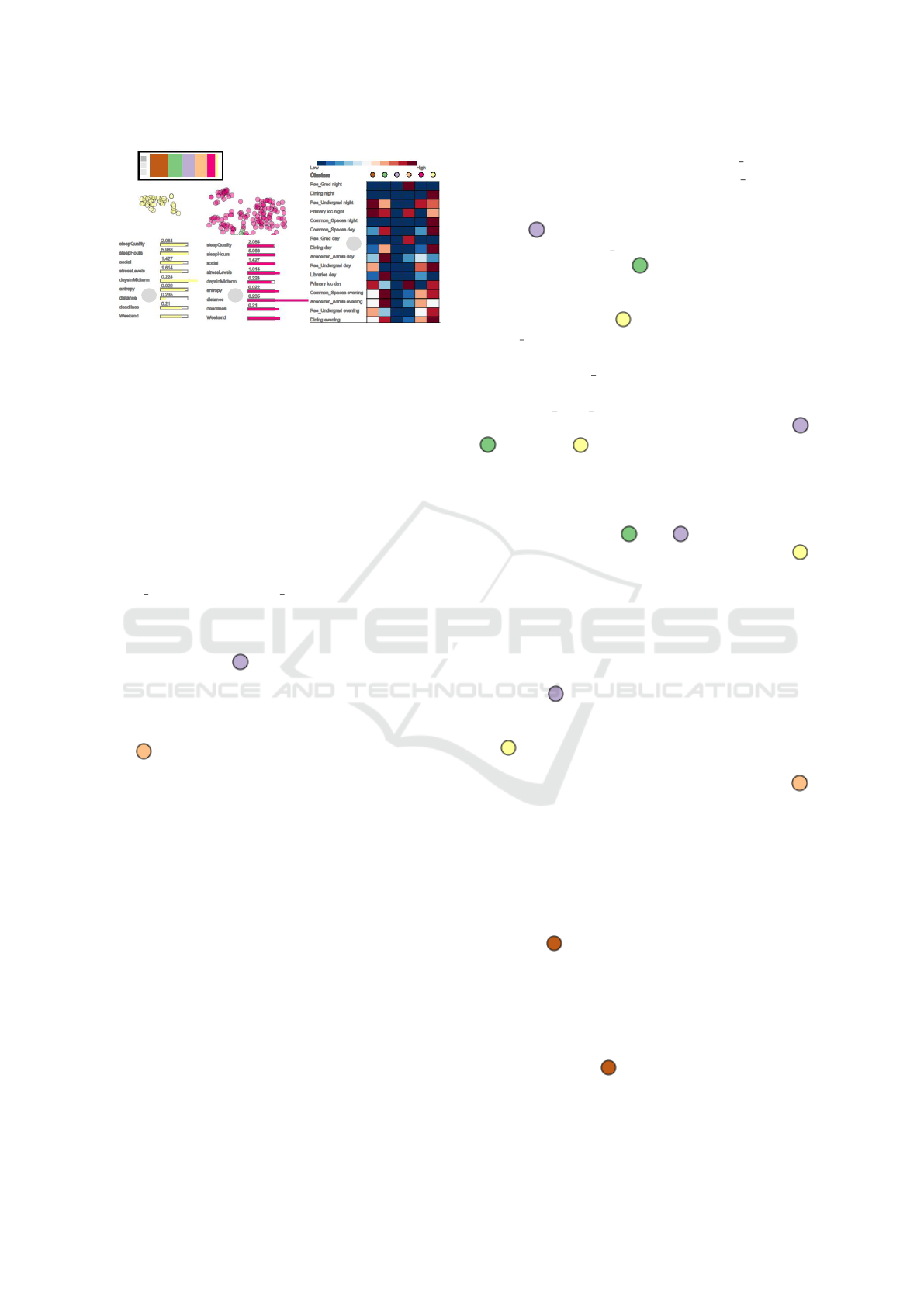
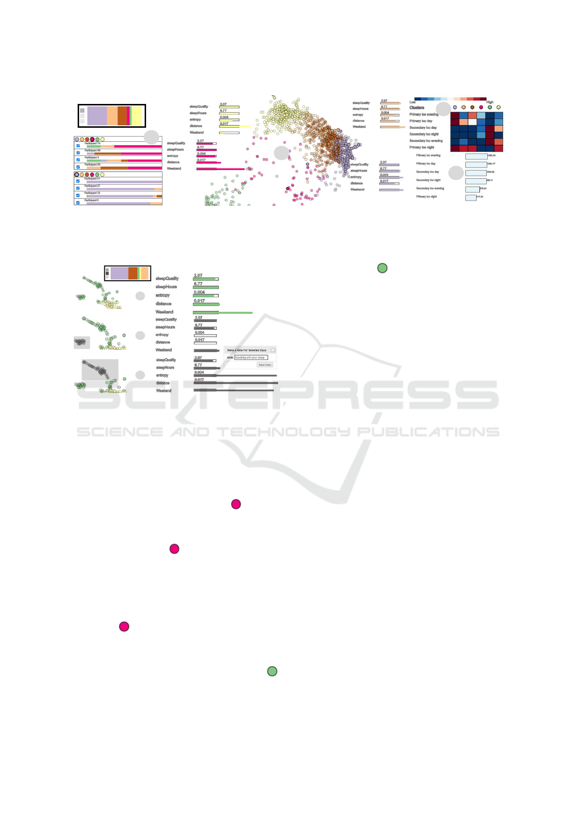
Figure 5: Visualizing ReadiSens data (dataset 2). A) Clustering the geo-features of the ReadiSens data with kMeans and

projecting it using Isomap. The yellow cluster has a much higher proportion of weekdays than other clusters along with

higher levels of distance travelled, perhaps indicating work-life routine. The pink cluster has days that are more likely to be

weekends and with lower sleep quality and little time spent in either the primary or the secondary locations.

Figure 6: A) The green cluster has 2 clumps. Days in this

cluster are more likely to be weekends than other clusters

and the sleep quality is poorer. B) Selecting the clump on

the left shows that those days are about as likely to be week-

ends as other clusters with average sleep quality and very

little travel. C) The clump on the right however has poorer

sleep quality and much more distance travelled. In addition

the days in this clump are much more likely to be weekends.

days can be used to identify future day level patterns.

Finally, she interacts with the cluster . Days in

this cluster are much more likely to be on weekends.

She notices in the FDH that there seem to be few in-

stances of participants being present in their primary

or secondary location for (Figure 5 B). In addition,

there seems to be a drop in the quality of sleep (G4,

T8). This along with its relatively small size leads

Luna to believe that this cluster represents days where

participants travelled. However, given that the cluster-

ing result is of poor quality (Figure 5 A) and the pro-

jection is scattered, she is unable to see a clear spatial

grouping of and decides to use other parameters.

She selects geo-features and tries t-SNE, kMeans

and k = 6. She selects a result with k = 5 clusters,

which has a better overall quality than the previous

selection (G1, T2, T3)(Figure 6) . She notices the

cluster (Figure 6 A) with higher than average days in

weekends and lower sleep quality. She notices two

separate clumps of and selects both of them sep-

arately using the “Selects Days” option (Figure 1 B)

to view their details. She notices that days in the ﬁrst

clump (Figure 6 B) are more likely to be on weekends,

with average sleep quality, lower sleep hours and little

movement across geo-locations (G4, T8, T9). Luna

takes a look at the next clump (Figure 6 C) and no-

tices that these days are far more likely to be week-

ends, register much higher than average distance trav-

elled and also contain poorer quality of sleep (G4, T8,

T9). She is conﬁdent that these days represent travel

and the context of knowing that these days are more

susceptible to lower quality sleep encourages Luna to

make classiﬁers to detect such behavior in future data

that may not contain any human provided labels. She

saves these days and their associated users as “travel-

ling with poor sleep” in the dialog that shows up after

the the days were brushed in the CV (G5, T10).

6 EVALUATION WITH EXPERTS

To evaluate PLEADES, we invited three evaluators

who were experts in building health predictive models

using machine learning and smartphone sensed data.

We also invited one expert in interactive data visual-

izations. We held a video-conference during which

the experts were free to contribute any feedback. Af-

ter a brief tutorial, they were led through the same use

cases as Luna. The experts were all well aware of un-

supervised clustering as a method for exploratory data

analysis. They liked the workﬂow of being able to se-

lect the sensor features and epochs, as they agreed that

during early exploration, they would need to use sev-

eral different parameters and algorithms before com-

ing across interesting results. They also found the

saving of results from previous analysis sessions to

be useful as they were aware of the computational

time complexity that can make cross clustering results

PLEADES: Population Level Observation of Smartphone Sensed Symptoms for In-the-wild Data using Clustering

comparisons time consuming.

One expert liked how we separated out the raw

sensor level data from the contextual data such as av-

erage sleep quality and proportion of days in week-

ends in the CDV as “it shows two types of information

like features that are maybe more granular and only

smartphone detectable and then you have this contex-

tual information that adds more semantic meaning.”

While going through the use cases, the experts

suggested potential groupings of users that we had

not considered. For instance, while going through use

case 2 (Section 5.3), they noticed that for the days

in cluster , there was little to no presence in on-

campus residences but presence in other on campus

buildings. There was also presence in the primary lo-

cation. This led the experts to believe that students

with days in this cluster may reside off-campus with

one expert suggesting grouping off-campus students

and on-campus students and clustering their data to

observe interesting changes in symptoms. For the

ReadiSens data (Section 5.6), one expert was curious

about comparing regular travellers with people who

stay home more as both these patterns can be predic-

tive of health issues (Weston et al., 2019). He sug-

gested ordering the users by

and (Figure 5 D).

After viewing the ordered list of users, he suggested

interest in selecting a sub-sample of users in the two

extremes and then computing a classiﬁcation model

to see if those users can be clearly separated out.

Overall, the evaluators liked PLEADES and

showed interest in using it to assign human under-

standable semantic labels to objective sensor data.

7 DISCUSSION AND

LIMITATIONS

The current research focus in smartphone-sensed

health monitoring is towards long-term deployment

of applications that can passively detect health. As

the number of participants increase along with longer

durations of participation, it may become difﬁcult to

analyze data on a per day basis on limited 2-D visual

real estate. Effective ﬁltering of participants along

with longer time windows such as weekly for binning

data may mitigate such issues. In addition, it may

be helpful to integrate such exploratory data analy-

sis with a machine learning pipeline that can use the

analyst selected days to classify patterns of interest.

For instance, taking the days labelled as “travelling

off campus” (end of Section 5.3) and selecting and

labelling another group of days when students were

on campus and using them as a training set to build a

classiﬁer. The various times of year can also be visu-

ally encoded, which can help analysts ﬁnd seasonal

patterns in reported symptoms.

8 CONCLUSION

We present PLEADES, an interactive visual ana-

lytics tool for exploratory analysis of smartphone

sensed data, to determine the contextual factors be-

hind the manifestation of smartphone inferred symp-

toms. PLEADES enabled the analysts to select clus-

tering and projection parameters such as the number

of clusters along with the clustering and dimension

reduction techniques and used multiple linked panes

containing visualizations like bar charts, heatmaps

and brushable parallel coordinated plots to present the

clustering results to allow users to link semantically

important information to objective smartphone sensed

data to further explain the human labelled symptom

reports. We validated our approach using two real

world datasets along with expert evaluation.

REFERENCES

Abdullah, S., Murnane, E. L., Matthews, M., and Choud-

hury, T. (2017). Circadian computing: sensing, mod-

eling, and maintaining biological rhythms. In Mobile

health, pages 35–58. Springer.

Boudjeloud-Assala, L., Pinheiro, P., Blansch

e, A., Tamisier,

T., and Otjacques, B. (2016). Interactive and it-

erative visual clustering. Information Visualization,

15(3):181–197.

Cali

nski, T. and Harabasz, J. (1974). A dendrite method for

cluster analysis. Communications in Statistics-theory

and Methods, 3(1):1–27.

Canzian, L. and Musolesi, M. (2015). Trajectories of de-

pression: unobtrusive monitoring of depressive states

by means of smartphone mobility traces analysis. In

Proceedings of the 2015 ACM international joint con-

ference on pervasive and ubiquitous computing, pages

1293–1304.

Cavallo, M. and Demiralp, C¸ . (2018). Clustrophile 2:

Guided visual clustering analysis. IEEE transactions

on visualization and computer graphics, 25(1):267–

276.

Chatzimparmpas, A., Martins, R. M., and Kerren, A.

(2020). t-visne: Interactive assessment and interpreta-

tion of t-sne projections. IEEE Transactions on Visu-

alization and Computer Graphics, 26(8):2696–2714.

Davies, D. and Bouldin, D. (1979). A cluster separation

measure, ieee transactions on patter analysis and ma-

chine intelligence. vol.

Ester, M., Kriegel, H.-P., Sander, J., Xu, X., et al. (1996).

A density-based algorithm for discovering clusters in

large spatial databases with noise. In Kdd, volume 96,

pages 226–231.

IVAPP 2021 - 12th International Conference on Information Visualization Theory and Applications

Fujiwara, T., Kwon, O.-H., and Ma, K.-L. (2019). Support-

ing analysis of dimensionality reduction results with

contrastive learning. IEEE transactions on visualiza-

tion and computer graphics, 26(1):45–55.

Gerych, W., Agu, E., and Rundensteiner, E. (2019). Clas-

sifying depression in imbalanced datasets using an

autoencoder-based anomaly detection approach. In

2019 IEEE 13th International Conference on Seman-

tic Computing (ICSC), pages 124–127. IEEE.

Harrower, M. and Brewer, C. A. (2003). Colorbrewer. org:

an online tool for selecting colour schemes for maps.

The Cartographic Journal, 40(1):27–37.

Hoque, E. and Carenini, G. (2015). Convisit: Interac-

tive topic modeling for exploring asynchronous on-

line conversations. In Proceedings of the 20th In-

ternational Conference on Intelligent User Interfaces,

pages 169–180.

Kwon, B. C., Eysenbach, B., Verma, J., Ng, K., De Filippi,

C., Stewart, W. F., and Perer, A. (2017). Clustervision:

Visual supervision of unsupervised clustering. IEEE

transactions on visualization and computer graphics,

24(1):142–151.

L’Yi, S., Ko, B., Shin, D., Cho, Y.-J., Lee, J., Kim, B.,

and Seo, J. (2015). Xclusim: a visual analytics

tool for interactively comparing multiple clustering

results of bioinformatics data. BMC bioinformatics,

16(S11):S5.

Maaten, L. v. d. and Hinton, G. (2008). Visualizing data

using t-sne. Journal of machine learning research,

9(Nov):2579–2605.

Madan, A., Cebrian, M., Moturu, S., Farrahi, K., et al.

(2011). Sensing the” health state” of a community.

IEEE Pervasive Computing, 11(4):36–45.

Mead, A. (1992). Review of the development of multidi-

mensional scaling methods. Journal of the Royal Sta-

tistical Society: Series D (The Statistician), 41(1):27–

39.

Mendes, E., Saad, L., and McGeeny, K. (2012).

https://news.gallup.com/poll/154685/stay-home-

moms-report-depression-sadness-anger.aspx.

Mohr, D. C., Zhang, M., and Schueller, S. M. (2017).

Personal sensing: understanding mental health using

ubiquitous sensors and machine learning. Annual re-

view of clinical psychology, 13:23–47.

Pu, J., Xu, P., Qu, H., Cui, W., Liu, S., and Ni, L. (2011).

Visual analysis of people’s mobility pattern from mo-

bile phone data. In Proceedings of the 2011 Visual In-

formation Communication-International Symposium,

page 13. ACM.

Ravesloot, C., Ward, B., Hargrove, T., Wong, J., Livingston,

N., Torma, L., and Ipsen, C. (2016). Why stay home?

temporal association of pain, fatigue and depression

with being at home. Disability and health journal,

9(2):218–225.

Restuccia, F., Ghosh, N., Bhattacharjee, S., Das, S. K., and

Melodia, T. (2017). Quality of information in mobile

crowdsensing: Survey and research challenges. ACM

Transactions on Sensor Networks (TOSN), 13(4):1–

43.

Rousseeuw, P. J. (1987). Silhouettes: a graphical aid to

the interpretation and validation of cluster analysis.

Journal of computational and applied mathematics,

20:53–65.

Sacha, D., Zhang, L., Sedlmair, M., Lee, J. A., Peltonen, J.,

Weiskopf, D., North, S. C., and Keim, D. A. (2016).

Visual interaction with dimensionality reduction: A

structured literature analysis. IEEE transactions on

visualization and computer graphics, 23(1):241–250.

Saeb, S., Zhang, M., Karr, C. J., Schueller, S. M., Corden,

M. E., Kording, K. P., and Mohr, D. C. (2015). Mo-

bile phone sensor correlates of depressive symptom

severity in daily-life behavior: an exploratory study.

Journal of medical Internet research, 17(7):e175.

Senaratne, H., Mueller, M., Behrisch, M., Lalanne, F.,

Bustos-Jim

enez, J., Schneidewind, J., Keim, D., and

Schreck, T. (2017). Urban mobility analysis with mo-

bile network data: a visual analytics approach. IEEE

Transactions on Intelligent Transportation Systems,

19(5):1537–1546.

Shen, Z. and Ma, K.-L. (2008). Mobivis: A visualization

system for exploring mobile data. In 2008 IEEE Pa-

ciﬁc Visualization Symposium, pages 175–182. IEEE.

Tenenbaum, J. B., De Silva, V., and Langford, J. C. (2000).

A global geometric framework for nonlinear dimen-

sionality reduction. science, 290(5500):2319–2323.

Vaizman, Y., Ellis, K., Lanckriet, G., and Weibel, N. (2018).

Extrasensory app: Data collection in-the-wild with

rich user interface to self-report behavior. In Proceed-

ings of the 2018 CHI Conference on Human Factors

in Computing Systems, pages 1–12.

Vetter, C. (2018). Circadian disruption: What do we actu-

ally mean? European Journal of Neuroscience.

Wang, R., Chen, F., Chen, Z., Li, T., Harari, G., Tignor, S.,

Zhou, X., Ben-Zeev, D., and Campbell, A. T. (2014).

Studentlife: assessing mental health, academic perfor-

mance and behavioral trends of college students using

smartphones. In Proceedings of the 2014 ACM inter-

national joint conference on pervasive and ubiquitous

computing, pages 3–14.

Wang, W., Mirjafari, S., Harari, G., Ben-Zeev, D., Brian,

R., Choudhury, T., Hauser, M., Kane, J., Masaba, K.,

Nepal, S., et al. (2020). Social sensing: Assessing so-

cial functioning of patients living with schizophrenia

using mobile phone sensing. In Proceedings of the

2020 CHI Conference on Human Factors in Comput-

ing Systems, pages 1–15.

Wenskovitch, J. and North, C. (2019). Pollux: Interac-

tive cluster-ﬁrst projections of high-dimensional data.

In 2019 IEEE Visualization in Data Science (VDS),

pages 38–47. IEEE.

Weston, G., Zilanawala, A., Webb, E., Carvalho, L. A.,

and McMunn, A. (2019). Long work hours, week-

end working and depressive symptoms in men and

women: ﬁndings from a uk population-based study.

J Epidemiol Community Health, 73(5):465–474.

PLEADES: Population Level Observation of Smartphone Sensed Symptoms for In-the-wild Data using Clustering