Optimal Distribution of CNN Computations on Edge and Cloud

Paul Albert Leroy and Toon Goedem

PSI-EAVISE, KU Leuven, Campus De Nayer, Belgium

Keywords:

Fog Computing, Edge, Cloud, CNN Model Partitioning.

Abstract:

In this paper we study the optimal distribution of CNN computations between an edge device and the cloud

for a complex IoT application. We propose a pipeline in which we perform experiments with a Jetson Nano

and a Raspberry Pi 3B+ as the edge device, and a T2.micro instance from Amazon EC2 as a cloud instance.

To answer this generic question, we performed exhaustive experiments on a typical use case, a mobile camera-

based street litter detection and mapping application based on a MobilenetV2 model. For our research, we

split the computations of the CNN model and divided them over the edge and cloud instances using model

partitioning, also including the edge-only and cloud-only conﬁgurations. We studied the inﬂuence of the

speciﬁcations of the instances, the input size of the model, the partitioning location of the model and the

available network bandwidth on the optimal split position. Depending on the choice of gaining either an

economic or performance advantage, we can conclude that a balance between the choice of instances and the

calculation mechanism used should be made.

1 INTRODUCTION

As artiﬁcial intelligence algorithms become more and

more complex and computationally demanding, for

every network-connected embedded application, one

of the most important design choices is where to run

the AI calculations: either on the edge device, or in

the cloud. Moreover, the choice is even more difﬁ-

cult, as one can imagine fog computing too, where the

calculations are distributed over both instances: a part

runs on the edge device, another part in the cloud. In

this paper we study which of these computing mech-

anisms (edge only, cloud only, split at an intermediate

position) is the most optimal, and which parameters

inﬂuence this optimum.

In order for conducting our research, we based

ourselves on (Loghin et al., 2019) and introduce a

pipeline consisting of an instance on the edge of the

network and an instance in the cloud. This gives

the opportunity of running computations on two lo-

cations, the edge device and the cloud instance.

Each of the two extremes have their speciﬁc ad-

vantages. When computations run on the cloud in-

stance solely, beneﬁts can be made since hardware re-

sources offered by a cloud provider are used instead

of using own acquired hardware. This means clients

don’t have to worry about complicated hardware and

its additional costs like electricity and purchase pric-

ing. The greatest advantage is the cloud’s scalability

and elasticity which give the opportunity of adding

additional instances or upgrading the speciﬁcations of

the used instances. Since all data needs to be trans-

mitted from the edge of the network to the cloud, in-

creased bandwidth, delay and security risk drawbacks

are introduced.

These drawbacks can be avoided by running all

the computations on the edge device of the pipeline.

Since the desired output of the computations is avail-

able in an earlier stage, the data can then be reduced

to speciﬁc harmless analysis results to send over caus-

ing that less information has to be sent over and thus a

decrease in previously stated drawbacks can be seen.

Despite this, hardware disadvantages emerge due to

the limited amount of resources available on an edge

device. These can be linked to trade-offs between

quality, cost and speed when designing the edge de-

vice.

In this paper, we study hybrid edge/cloud com-

puting where computations are spread over both in-

stances. We want to examine whether a distribu-

tion of computing between edge and cloud can ob-

tain any economical or performance beneﬁts. The re-

search question of this paper is as follows: which pa-

rameters determine the optimal distribution between

edge- and cloud computing to maximise beneﬁts?

The used computations originate from a convolutional

neural network which will be split between a certain

layer position. Using this method, the two resulting

604

Leroy, P. and Goedemé, T.

Optimal Distribution of CNN Computations on Edge and Cloud.

DOI: 10.5220/0010203706040613

In Proceedings of the 13th International Conference on Agents and Artiﬁcial Intelligence (ICAART 2021) - Volume 2, pages 604-613

ISBN: 978-989-758-484-8

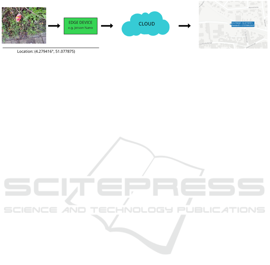
Figure 1: Application pipeline: The device located at the edge of the network captures images and geographical information.

This is then sent over to the cloud which visualises it. Computing can be done on the edge device and the cloud.

submodels can be deployed on the two available in-

stances. By splitting in between various layers, sev-

eral submodels with each a different amount of com-

putations are tested. We also study the effects of scal-

ing this approach to multiple users.

The experiments for this study are based on a use

case in which an image processing algorithm deter-

mines whether or not litter is present in a camera im-

age, captures the geographical coordinates of it, and

eventually visualises it on a map as seen in ﬁgure 1.

The remainder of this paper is structured as fol-

lows. Section 2 gives an overview of related work on

hybrid edge/cloud computing. In section 3 we dis-

cuss the litter detection use case and our chosen CNN

model. The approach of realising our pipeline and the

used computation splitting method can be found in

section 4. Results of conducted experiments are eval-

uated in section 5. Conclusions follow in section 6.

2 RELATED WORK

In (Loghin et al., 2019), experiments were done on

a variety of well-known computing applications (ex-

cluding CNN), one computationally more demanding

than the other. The authors conclude that computing

on cloud is usually faster than edge-only, but coun-

terbalanced by the latency of sending over data to the

cloud. They also state that hybrid edge/cloud-only has

beneﬁts when not a lot of bandwidth is available, and

the application uses a large input with small interme-

diate results. The paper overall stated that a beneﬁt in

speed performance depends on the speciﬁcations of

the used application and the available bandwidth.

More related to our research is Deepdecision (Ran

et al., 2018) as their computations also are derived

from a CNN. This work proposes a method called

ofﬂoading with the purpose of gaining accuracy and

framerate. The system uses a larger CNN running on

the cloud and a smaller CNN running on the edge.

With ofﬂoading, a decision is made on the edge par-

tition whether to use the smaller local convolutional

neural network or send over the data to the cloud. This

decision is based on variables like available band-

width, required accuracy, etc. In contrary to our work,

the CNN runs solely on a single instance.

(Teerapittayanon et al., 2017b) proposed dis-

tributed deep neural networks (DDNNs) which show

similarities with Deepdecision. In their work, a reduc-

tion of communication cost is achieved by a factor of

over 20x as oppose to cloud-only computing. Based

on their earlier work Branchynet(Teerapittayanon

et al., 2017a), the number of computations done by

a neural network can be decreased with the introduc-

tion of early exit points. These points create the pos-

sibility of classifying samples in an earlier stage of

the network by adding a classiﬁer in between inter-

mediate layers. An entropy-based conﬁdence crite-

rion decides whether or not any further computations

have to be applied by the following layers of the net-

work. DDNN beneﬁts from this concept by applying

it in a pipeline and partition the model over edge and

cloud. Primary layers of the NN, in conjunction with

an exit point, are deployed on the edge device. On

the edge instance, the decision is made whether ad-

ditional computations is needed due to the lack of the

prediction’s conﬁdence. If not, the intermediate result

is sent over and further computations are executed by

the remaining part of the neural network on the cloud.

In this paper, we base our pipeline architecture

on (Loghin et al., 2019), but extend it towards con-

volutional neural networks and see of their conclu-

sions hold. To spread our computations, we use a

simpliﬁed method of the one introduced in (Teerapit-

tayanon et al., 2017b): instead of adding an interme-

diate classiﬁer, we plainly split the CNN model into

two submodels and deploy these individually on two

instances.

3 LITTER DETECTION USE

CASE

To give this research an additional useful purpose, we

chose a use case on which we based our experiments

Optimal Distribution of CNN Computations on Edge and Cloud

605

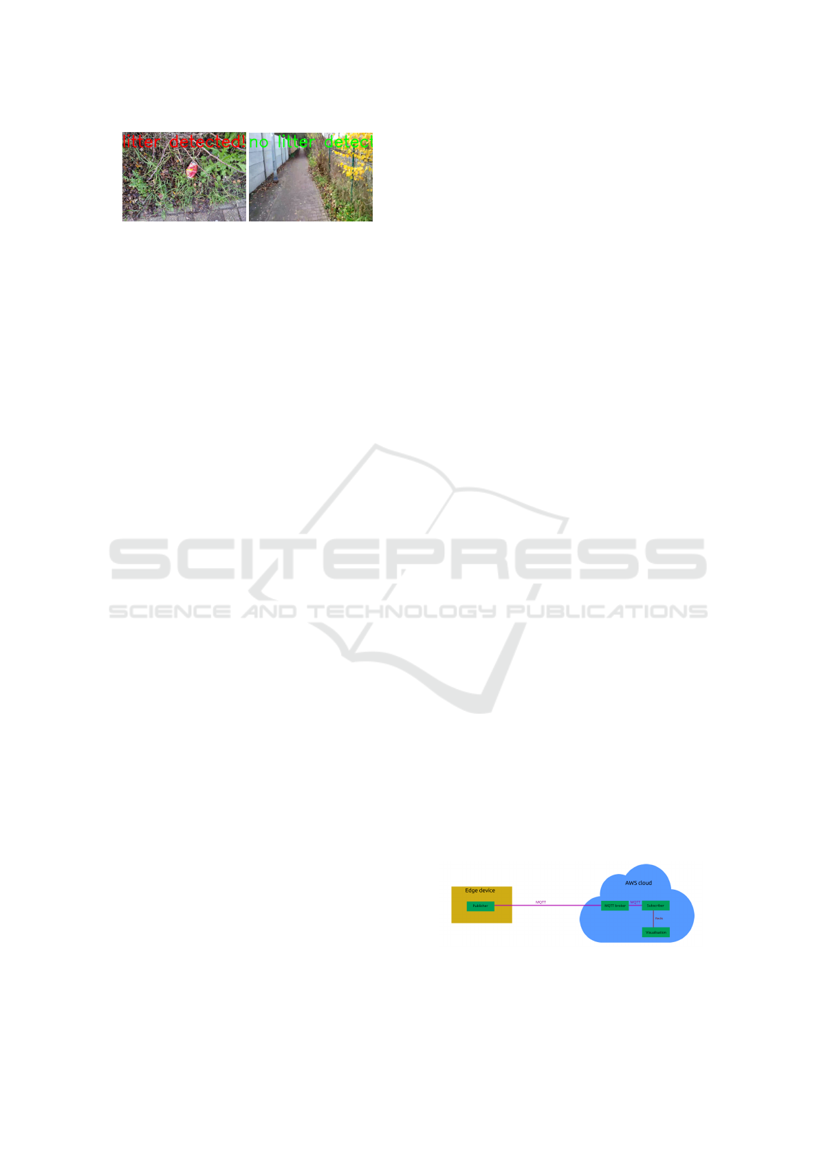
Figure 2: Examples of our trained model making predic-

tions about the presence of litter in the image.

on. The idea for this arose from a problem humanity

is confronted with globally: litter. Virtually every-

where you walk or bike around on this planet, you

can see trash, such as paper, cans, and bottles, that is

left lying on the ground. We work towards a mobile

embedded device that detects litter in its camera im-

ages, capture the geographical coordinates of it and

eventually visualise it on a map. With many users

in parallel, a quick litter density mapping of a large

region can be obtained, yielding important input for

efﬁcient cleanup operations.

3.1 Neural Network Architecture

Previous work (Mittal et al., 2016; Vo et al., 2019)

show that the majority of proposed techniques for lit-

ter detection, often rely on convolutional deep neural

networks. For realising the use case, we chose to train

a convolutional neural network for classiﬁcation in-

stead of object detection. As we only know the GPS

position of the mobile device taking the litter photos,

and not the orientation of it, information about the lo-

cation of the litter in the image has no added value in

our use case.

During the experiments of this paper, we want

to compare different hybrid edge/cloud splits to the

cloud-only and edge-only extremes. Therefore we

need to take into account that a CNN architecture

needs to be chosen which is capable of running

entirely on an edge device with limited resources.

Two of the most promising architectures are the

well-known MobilenetV2(Sandler et al., 2018) and

YOLOv2(Redmon and Farhadi, 2016). The main dif-

ference is that MobilenetV2 is a network used for

classiﬁcation, whereas YOLOv2 is used for object de-

tection. Since object detection does not have any ben-

eﬁt in our use case as described above, our preference

goes to MobilenetV2. This lightweight architecture

offers fairly good accuracy and fast inference speeds

for a minimal amount of operations, thus making it

possible to run on devices with limited resources (e.g.

Raspberry Pi).

3.2 Training

We selected the Garbage In Images dataset (GINI)

(Mittal et al., 2016) to train our network on. It pro-

vides us with the required classes: garbage-queried-

images and non-garbage-queried-images. GINI con-

tains 907 images of scenes with litter and 1605 images

where litter is not present.

To train our network we utilised Tensorﬂow 2.0.0

and Keras and performed transfer learning from a Mo-

bilenetV2 model pre-trained on ImageNet. We ﬁrst

trained our classiﬁcation layers using 20 epochs, and

then ﬁne-tuned our model for 10 epochs to increase

the accuracy. Additionally, as is described in section

5, we want to test if the image input size inﬂuences

the latency. In order to do this, we trained two mod-

els with different input size: 160 × 160 and 224 × 224

pixels. Figure 2 shows example predictions of our

trained model on self captured data.

4 APPROACH

The goal of this paper is to identify which parame-

ters inﬂuence the most advantageous choice of how

to distribute CNN computations over an edge device

and the cloud. These advantages can be economically

or in terms of performance. In this section, we ex-

plain our test setup to conduct experiments on. We

will ﬁrst (section 4.1) present the pipeline we de-

signed which uses computations of our self-trained

MobilenetV2 model. In order to divide our compu-

tations and spread these over the available instances,

we used a model partitioning procedure explained in

section 4.2.

4.1 Pipeline

For this paper we developed a pipeline, based on the

one used in (Loghin et al., 2019), but altered to our

use case (see ﬁgure 3 for an overview). Notice the

two instances where computations can be done, the

edge and the cloud. This gives us the possibility of

applying the three different computing mechanisms

Figure 3: Overall pipeline designed for our research.

Docker containers run on the edge instance (Raspberry Pi

or Jetson Nano) and cloud instance (T2.micro).

ICAART 2021 - 13th International Conference on Agents and Artiﬁcial Intelligence

606

discussed in section 1. We further discuss the imple-

mented instances ﬁrst.

A large variety of instances can be chosen to be

placed on the edge of the device depending on the ap-

plication. When choosing our edge device we want to

use, we needed to keep in mind that the possibility of

running deep learning architectures on the device was

possible. We decided to compare two edge devices in

this study: Jetson Nano and Raspberry Pi. In table 1

an overview of speciﬁcations from both can be seen.

We can see that the Jetson Nano is equipped with a

very powerful GPU as opposed to the Raspberry Pi.

This is due to the fact that the Nano is designed with

the main purpose of running machine learning algo-

rithms, which can be noticed on the AI Performance

speciﬁcation. We observe that this compute perfor-

mance is a trade-off with device cost. For this rea-

son, we want to compare it with a less powerful, but

cheaper alternative. We have decided to go with the

popular Raspberry Pi, model 3B+ in particular.

For our cloud instance we conﬁgured a t2.micro

instance provided by Amazon Web Services. Due

to our limited budget costs, we decided to use AWS

since it offers an AWS educate programme. Speciﬁ-

cations of the used instance can be found in table 2.

As we notice, the cloud instance is capable of reach-

ing higher clock speeds opposite to the chosen edge

devices.

During the development of this test setup, we

have taken advantage of Docker containers. This

simpliﬁes the task of deploying and running applica-

tions independent from the used operating system. In

our pipeline, we created four containers: publisher,

MQTT broker, subscriber and a visualisation con-

tainer. The communication between these is estab-

lished using the MQTT (Message Queuing Telemetry

Transport) protocol. Our ﬂow begins with the pub-

lisher on the Edge device which is responsible for

collecting image data, resizing it to the appropriate in-

put size, if needed processing the data using a model,

and eventually parsing our data to JSON format. The

choice of data we need to send over depends on the

computing mechanism we are applying. For exam-

ple the cloud-only mechanism needs data of the entire

image to transfer, while for the splitted networks, an

intermediate activation tensor must be transferred.

Our JSON data is sent over to another container

which is running an instance called a broker. The ob-

jective of the broker is to handle incoming and outgo-

ing data messages sent over MQTT, we need to run

this application in the cloud since it needs to han-

dle the messages of multiple edge devices. Running

alongside the broker is a container holding a sub-

scriber application. MQTT messages of multiple pub-

lishers, hence multiple edge devices, are received by

this application. When receiving the data, the sub-

scriber decodes the JSON, if needed run a model to

make a prediction for the received information, and

saves this data. The end objective of our use case is to

use the information we have gathered to visualise the

litter locations on a map. For this task, we uilised the

Plotly Dash framework. To communicate with this

container, Redis is used since using the application

as MQTT subscriber simultaneously gave problems.

The map is automatically updated when new data is

added by the MQTT subscriber.

4.2 Model Partitioning

We selected a number of places, spread over the Mo-

bilenetV2 architecture, where we could to split the

model. As we can see on ﬁgure 4 plots the size of

the intermediate activation tensor of the CNN when

using a 160 × 160 pixels input architecture, and the

14 points where we will try to split it. The decision

of a certain point is based on how much information

is outputted by the previous layer, to be sent over to

the second partition of the model which is located

in the cloud. It is evident that we want to minimise

the amount of data sent over. Usually, these places

occur between two overall bottleneck blocks or in-

side a linear bottleneck block. This is no coincidence

since it is logical to not split inside an inverted resid-

ual block. As we can read in (Sandler et al., 2018),

we can conclude that the data of the ﬁrst link layer’s

output also is needed by the next layers on the sec-

ond part of the model. This introduces the drawback

of sending over more data. We have chosen a vari-

ety of split points spread over the whole architecture

of MobilenetV2 since we want to research the model

partitioning method with the interest of obtaining any

beneﬁts economically or performance-wise.

To analyse these split points theoretically, we

counted the amount of Multiply-Add operations each

resulting submodel of the CNN architecture needs.

This is a coarse approximation of the ﬂops needed

by each submodel, as one Multiply-Add can be ap-

proximated as two ﬂops. The calculated

amount of

MAdds for each layer are visualised in ﬁgure 5.

5 EVALUATION

In this section, we describe the experiments we

conducted to research the performance advantages.

These were performed on the pipeline we introduce

https://machinethink.net/blog/how-fast-is-my-model/

Optimal Distribution of CNN Computations on Edge and Cloud

607

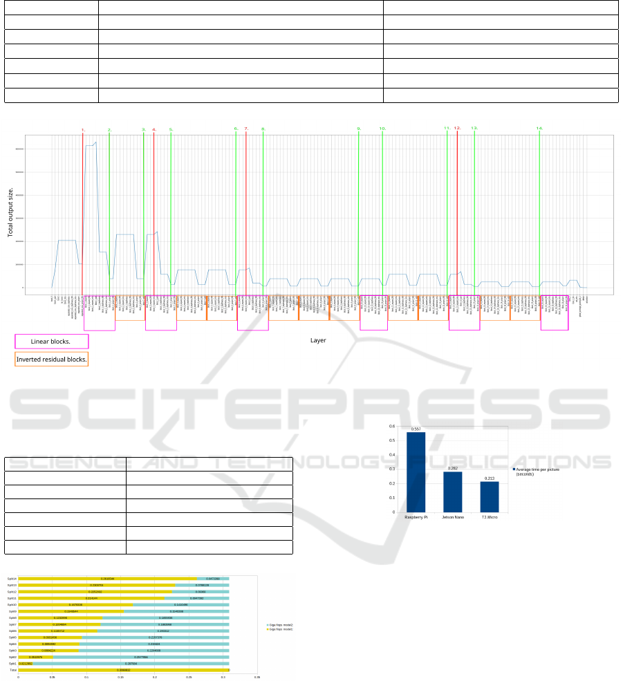
Table 1: Speciﬁcations of the Jetson Nano and the Raspberry Pi 3B+.

Speciﬁcation Jetson Nano Dev Board Raspberry Pi 3B+

AI Performance 472 GFLOPs 21.4 GFLOPs

GPU 128-core NVIDIA Maxwell Broadcom VideoCore IV

CPU 1.4 GHz 64-bit Quad-Core ARM Cortex-A57 MPCore 1.4 GHz 64-bit quad-core ARM Cortex-A53

Power usage P 5 to 10 Watts 1.7 to 5.1 Watts

RAM 4GB LPDDR4 1GB LPDDR2 SDRAM

Price per device ±e122 ±e40

Figure 4: MobilenetV2 architecture with input size 160 × 160: output size of every layer plotted, as well as the linear and

inverted residual blocks. Vertical lines are proposed CNN split points.

Table 2: T2.micro instance speciﬁcations and pricing. The

instance is equipped with a powerful CPU.

Speciﬁcation t2.micro:

vCPU 3.3 GHz Intel Scalable Processor

RAM (GiB) 1.0

CPU Credits/hr 6

On-Demand Price/hr $.0116 = e.01

1-yr Reserved Price/hr $.007 = e.0062

3-yr Reserved Price/hr $.005 = e.0044

Figure 5: Total Giga ﬂops for each splitted model. Yellow:

edge, blue: cloud.

in section 4.1. For each test we used the same 40 test

pictures, with associated geographical data, read in by

the edge instance, being respectively a Jetson Nano

or a Raspberry Pi. These send data over to the AWS

t2.micro cloud instance. The content of this data de-

pends on the mechanism as we explained in section

4.1. We timed every interesting stage of the pipeline,

Figure 6: Average time for predicting single picture when

running the 160 × 160 model solely on each available in-

stance.

and measured these using the partitioned models de-

scribed in section 4.2 as well as running the entire

model on the edge or cloud individually. One of the

advantages of edge-only computing is that we do not

need to send over all our data. We apply this in our

case study by only sending over the data of images

containing litter, thus sending over fewer data to the

cloud. For each of the split positions, the amount of

data sent over depends on the size of the activation

tensor of the CNN at the chosen point (see ﬁg. 4).

5.1 Processing Time Experiments

Various parameters were observed during our exper-

iments including: different computing mechanisms,

varying the image resolution and networks with dif-

ICAART 2021 - 13th International Conference on Agents and Artiﬁcial Intelligence

608

ferent bandwidths.

During the analysis of the results we gathered, we

noticed that the time, data sits in the waiting queue

of MQTT to be sent over, is not consistent. Because

it is an obvious future work optimisation to make

sure queue waiting times are minimal, we neglect

this waiting time in our measurements. Therefore we

will report below all latencies as ”Hypothetical Total

Per Image”, where we neglect the waiting time in the

queue.

5.1.1 Individual Processing Power of Edge and

Cloud Instances

Since each of the instances we used has various spec-

iﬁcations, hence different performances, it may be in-

teresting to inspect these individually. Figure 6 shows

the average inference time we measured of each in-

stance. We observe that the cloud has the fastest in-

ference time, followed by the GPU-powered Jetson

Nano.

5.1.2 Inﬂuence of the Computing Mechanism

In the ﬁrst experiment we conducted, we wanted to

discover whether a split architecture has any perfor-

mance beneﬁts. We visualise our measured results

in ﬁgure 7 for the 160×160 model. When we anal-

yse our measurements, we observe that overall a par-

titioned model has a better performance in compari-

son to cloud-only. In both cases, a split model is the

fastest among the researched models. The reason for

this is probably the fact that the size of the interme-

diate data is smaller than the input size when com-

paring it with the cloud-only mechanism. Edge-only

also shows great results, but this is overshadowed due

to the computing power of the cloud.

5.1.3 Inﬂuence of the Image Resolution

Another parameter which could affect the perfor-

mance is the input size of the used model. When

adjusting the input size, the output size of all inter-

mediate layers changes simultaneously. When study-

ing our results in ﬁg.8, we can conclude the Jetson

is faster due to its GPU performance. More interest-

ing is when we compare these results with previous

results for a 160 × 160 model found in ﬁgures: 7a

and 7b, we notice a decrease in time performance.

This can be linked to two occurrences in our mea-

sured data. To start off, we observe that the prediction

time of our model will increase when the input size is

increased. We can see this phenomenon both on the

edge and cloud side. Additionally, a second reason for

the increase in our total measured latency the increase

in sending over time, due to the increased amount of

data to be sent over.

When reviewing the total latency per image, we

notice that the Jetson Nano beneﬁts most with split13.

This behaviour can be linked to the small intermedi-

ate activation tensor of split13 as seen in ﬁgure 4. The

Raspberry has more advantage when sending over the

resized input to the cloud. When comparing this with

split13, we notice the relatively fast prediction times

of the cloud counterbalances the slower prediction

times of the Raspberry Pi.

5.1.4 Inﬂuence of the Network Speed

We have to keep in mind that in the future, our use

case application will run on portable edge devices.

This means in order to have a connection with the

cloud, a mobile network must be used, e.g. 4G. The

disadvantages with these are the limited upload and

download speeds. For this reason, it is interesting

to research whether these setbacks have any conse-

quences that inﬂuence our speed performance. Mea-

surements are visualised in ﬁgure 9. As expected we

can see our send over times increase due to slower up-

load speed leading to edge only being the better per-

forming mechanism.

5.2 Economical Model

The purpose of this paper is to research whether we

can gain any beneﬁts by utilising this pipeline with

different instances and splitting mechanisms. The op-

timal choice, however, depends on the optimisation

criterium: calculation speed performance or total eco-

nomical cost. As in many cases, these two form a

trade-off.

When speed performance is very important, for

example for a monitoring system for a dangerous

industrial process, our experiments described above

suggest that the best choice is using a pipeline with

a powerful edge device. If a normal or high amount

of bandwidth is available, a split model might be the

best option. When in a case with limited bandwidth,

we are better off with running the entire model on

the edge and only send over the necessary data to the

cloud. In this situation, we have a big economical

drawback since powerful edge devices cost a lot of

money and have large power consumption as can be

seen in table 1. When the costs need to be minimised,

a cheaper edge device can be used, but latency will in-

crease as seen in the test results. To know where this

trade-off lies, in this section we will calculate an esti-

mated cost for the different computing mechanisms of

our test case at hand, the MobilenetV2 litter detection

application.

Optimal Distribution of CNN Computations on Edge and Cloud

609

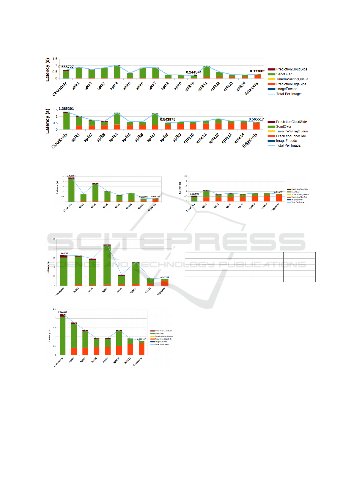
(a) Measured latency for Jetson Nano.

(b) Measured latency for Raspberry Pi.

Figure 7: Measured timings with 160×160 model.

(a) Measured latency for Jetson Nano. (b) Measured latency for Raspberry Pi.

Figure 8: Measured latencies with 224 × 224 model.

(a) Measured latency for Jetson Nano.

(b) Measured latency for Raspberry Pi.

Figure 9: Measured latencies with 224 × 224 model using

4G.

We ﬁrst clarify the costs between using a cheap and

expensive edge device. We take worst-case values

for power consumption: the energy prices for Belgian

companies in April 2020 (e0.20/kWh). In table 3, we

Table 3: Comparing costs between the Jetson Nano and the

Raspberry Pi.

Jetson Nano Raspberry Pi

Purchase price ±e122 ±e40

Energy usage E 0.01kW 0.0051kW

Energy costs/hour e0.002 e0.001

Energy costs/month per device e1.46 e0.73

calculated the total price for purchasing a device and

running it one month. As we can tell from the results,

using a more powerful edge device can almost triple

the costs in worse case scenarios.

Not only the choice of the edge device makes a

difference. When multiple users are deployed simul-

taneously, the computing cost of the instance in the

cloud and the choice of the used mechanism need to

be taken into account. This is due to the different

amounts of cloud processing power usage across var-

ious mechanisms.

Applied to our test case, let assume we have 5000

edge devices running simultaneously for a month’s

time, which are connected to the same t2.micro in-

stance as used in the example with a limited CPU load

of 95%. Speciﬁcations of this instance can be found

in table 2. For this example, we measured the com-

puting power usage of the cloud for various choices

of computing mechanisms and calculated the required

amount of instances needed for 5000 edge devices.

ICAART 2021 - 13th International Conference on Agents and Artiﬁcial Intelligence

610

Table 4: Example calculation of cloud processing costs for

5000 users for the computing mechanisms. (Hardware and

energy cost of the edge devices is not taken into account).

Cloud only Edge only Split5 Split10 Split13

#users/instance 10 228 29 32 143

#instances

total

500 22 173 157 35

total costs/month e3763.5 e165.594 e1302.171 e1181.739 e263.445

monthly costs/user e0.7526 e0.0331 e0.2604 e0.2363 e0.0526

Also, we calculated the costs of running the t2.micro

instance for these 5000 users for a month were calcu-

lated. Results are listed in table 4.

As we can see in table 4, pricing can change dras-

tically depending on the used computing mechanism.

We notice that the costs depend on the number of

needed instances, thus on the maximum amount of

users per instance. When we combine the results of

table 3 and table 4, we can calculate the total costs

per month for the global pipeline. Results of these

costs can be found in table 5 for the Jetson Nano and

table 6 for the Raspberry Pi. We assume that the de-

vices keep functioning one year, such that the pur-

chase cost of the edge hardware needs to be venti-

lated over 12 months. As previously mentioned, we

can see a huge difference between the various com-

puting mechanisms. Another noticeable fact, which

we already noticed in table 3, is the huge difference in

expenses depending on the used edge device. These

originate from the energy costs difference and the to-

tal costs of purchasing 5000 devices.

We can conclude that a balance needs to be found

between the costs of the edge device and the used

mechanism depending on the requirements of the ap-

plication. For example, when using an edge-only

method we can see cloud costs are minimal, but as

stated earlier a splitted model may have more speed

performance beneﬁts. This beneﬁt has the disadvan-

tage of a higher monthly cost due to the higher CPU

usage of the cloud. This trade-off between time per-

formance and cost is visualised in ﬁg. 10. It is re-

markable that indeed for different situations, differ-

ent distribution mechanisms are optimal. We observe

that, for smaller edge devices, edge-only computation

is the cheapest and the fastest solution for this net-

work, while for larger devices a middle split between

edge and cloud is preferable.

6 CONCLUSION

In this paper, we studied which parameters determine

the optimal distribution of CNN computations be-

tween edge and cloud computing to maximise speed

and performance beneﬁts. In order to answer this

question we studied a practical use case, the detec-

tion of litter on a ﬂeet of cloud-connected embedded

devices. We trained a MobilenetV2 CNN model, and

performed experiments on a self designed pipeline in

which we splitted this CNN model over the edge and

cloud instances.

We ﬁrst conducted research on the three differ-

ent instances separately. Our used instances were two

possible edge devices: a Jetson Nano and a Raspberry

Pi, and the cloud. These each have distinctive speciﬁ-

cations, hence different performance values.

In our experiments, we splitted the MobilenetV2

architecture between the convolution layers. We com-

pared these partitioned models with ordinary comput-

ing mechanisms (egde-only and cloud-only) by tim-

ing each interesting process of the pipeline. When

analysing the tests done on the 160 × 160 model, we

can see a partitioned model has more gain in ben-

eﬁts. This behaviour can be linked to the amount

of data sent over. We observed that edge comput-

ing can reduce latency by sending over less data, but

this is counterbalanced by the computing power of the

cloud.

For a larger input image size, 224×224, the model

gave different results. The obvious difference we ﬁrst

notice is the prediction times on both the edge and

the cloud increased. Due to the change in input size

of the neural network, intermediate activation tensor

sizes change simultaneously. Because of this split13

becomes the fastest choice for the Jetson Nano as op-

posed to the 160 × 160 model. Because of the weaker

computational performance of the Raspberry Pi and

the good computing power of the cloud, the fastest

mechanism is ofﬂoading this larger model to the cloud

and sending over the resized input image.

As we see that sending intermediate results over

the network consumes a substantial amount of the to-

tal latency, we investigated the inﬂuence of the speed

of this network. We conclude that networks with lim-

ited speciﬁcations (like 4G) indeed have an impact

on the performance of the pipeline. The most bene-

ﬁcial mechanism for this situation is running the en-

tire model on the edge device, indeed sending over the

least amount of data.

Next to an optimisation towards maximal speed

performance, we also studied the economical cost

of each mechanism, an optimisation criterium that

is orthogonal to performance. When speed is im-

portant, we can conclude a high bandwidth together

with a splitted mechanism and a powerful but expen-

sive edge device is recommended. Economically, our

choice of the used mechanism makes a huge differ-

ence in expenses. From our detailed cost estimate,

we can state that when the CPU usage of the cloud in-

creases, costs will increase simultaneously since more

instances are needed to divide the workload. This

Optimal Distribution of CNN Computations on Edge and Cloud

611

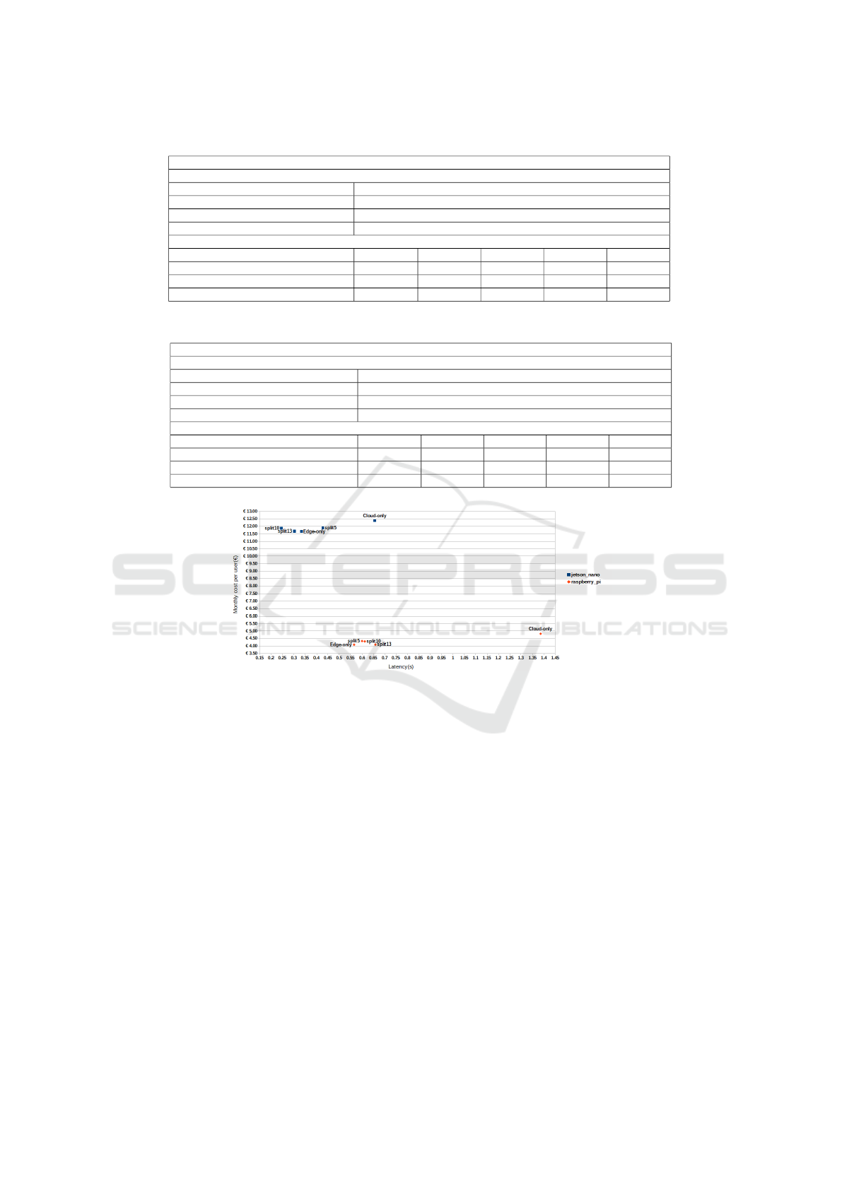
Table 5: Total costs between the various computing mechanisms with a Jetson Nano edge instance.

Jetson Nano

Edge device costs:

Total purchase price for 5000 devices e610000

Purchase per month spread over 1 year e50833.333

Energycosts

device

/month e7300

Total for edge device: e58133.333

Cloud costs:

Cloud-only Edge-only Split5 Split10 Split15

Cloud costs/month e3763.5 e165.594 e1302.171 e1181.739 e263.445

Total cost per month e61896.83 e58298.93 e59435.5 e59315.07 e58396.78

Total monthly cost per user e12.37 e11.66 e11.88 e11.86 e11.67

Table 6: Total costs between the various computing mechanisms with a Raspberry Pi edge instance.

Raspberry Pi

Edge device costs:

Total purchase pricing for 5000 devices e200000

Purchase per month spread over 1 year e16666.667

Energycosts

device

/month e3650

Total for edge device: e20316.667

Cloud costs:

Cloud-only Edge-only Split5 Split10 Split15

Cloud costs/month e3763.5 e165.594 e1302.171 e1181.739 e263.445

Total cost per month e24080.17 e20482.26 e21618.84 e21498.41 e20580.11

Total monthly cost per user e4.816 e4.096 e4.324 e4.300 e4.116

Figure 10: Monthly costs per user w.r.t. the latency for the 160×160 model and standard network bandwidth.

means a more powerful cloud instance can also make

a difference. In this paper we used two edge devices

from different price classes, resulting in a huge to-

tal cost difference.Remarkable, for the more expen-

sive device we notice a partitioned mechanism is the

best trade-off when both performance and total cost

are taken into account.

The overall conclusion is that indeed a balance

needs to be found between the choice of the edge de-

vice and the decision of the used splitting mechanism.

This balance is based on the criterion in which we

want to gain beneﬁts. In our case study, the edge-only

mechanism appears to be the cheapest, a split model

has the best beneﬁt in speed performance.

ACKNOWLEDGEMENTS

This work is supported by VLAIO and Klarrio via the

Start to Deep Learn TETRA project.

REFERENCES

Loghin, D., Ramapantulu, L., and Teo, Y. M. (2019).

Towards analyzing the performance of hybrid edge-

cloud processing. In 2019 IEEE Intl. Conf. on Edge

Computing (EDGE), pages 87–94. IEEE.

Mittal, G., Yagnik, K., Garg, M., and Krishnan, N. (2016).

Spotgarbage: smartphone app to detect garbage using

deep learning. In Proceedings of the 2016 ACM In-

ternational Joint Conference on pervasive and ubiqui-

tous computing, UbiComp ’16, pages 940–945. ACM.

Ran, X., Chen, H., Zhu, X., Liu, Z., and Chen, J.

(2018). Deepdecision: A mobile deep learning frame-

ICAART 2021 - 13th International Conference on Agents and Artiﬁcial Intelligence

612

work for edge video analytics. In IEEE INFO-

COM 2018-IEEE Conference on Computer Commu-

nications, pages 1421–1429. IEEE.

Redmon, J. and Farhadi, A. (2016). Yolo9000: Better,

faster, stronger.

Sandler, M., Howard, A., Zhu, M., Zhmoginov, A., and

Chen, L.-C. (2018). Mobilenetv2: Inverted residuals

and linear bottlenecks.

Teerapittayanon, S., McDanel, B., and Kung, H. T. (2017a).

Branchynet: Fast inference via early exiting from

deep neural networks.

Teerapittayanon, S., McDanel, B., and Kung, H. T. (2017b).

Distributed deep neural networks over the cloud, the

edge and end devices.

Vo, A. H., Hoang Son, L., Vo, M. T., and Le, T. (2019).

A novel framework for trash classiﬁcation using deep

transfer learning. IEEE Access, 7:178631–178639.

Optimal Distribution of CNN Computations on Edge and Cloud

613