Indoor Point-to-Point Navigation with Deep Reinforcement Learning and
Ultra-Wideband
Enrico Sutera
1,2 a
, Vittorio Mazzia
1,2,3 b
, Francesco Salvetti
1,2,3 c
, Giovanni Fantin
1,2 d
and Marcello Chiaberge
1,2 e
1
Department of Electronics and Telecommunications, Politecnico di Torino, 10124 Turin, Italy
2
PIC4SeR, Politecnico di Torino Interdepartmental Centre for Service Robotics, Turin, Italy
3
SmartData@PoliTo, Big Data and Data Science Laboratory, Turin, Italy
Keywords:
Indoor Autonomous Navigation, Autonomous Agents, Deep Reinforcement Learning, Ultra-Wideband.
Abstract:
Indoor autonomous navigation requires a precise and accurate localization system able to guide robots through
cluttered, unstructured and dynamic environments. Ultra-wideband (UWB) technology, as an indoor position-
ing system, offers precise localization and tracking, but moving obstacles and non-line-of-sight occurrences
can generate noisy and unreliable signals. That, combined with sensors noise, unmodeled dynamics and
environment changes can result in a failure of the guidance algorithm of the robot. We demonstrate how
a power-efficient and low computational cost point-to-point local planner, learnt with deep reinforcement
learning (RL), combined with UWB localization technology can constitute a robust and resilient to noise
short-range guidance system complete solution. We trained the RL agent on a simulated environment that
encapsulates the robot dynamics and task constraints and then, we tested the learnt point-to-point navigation
policies in a real setting with more than two-hundred experimental evaluations using UWB localization. Our
results show that the computational efficient end-to-end policy learnt in plain simulation, that directly maps
low-range sensors signals to robot controls, deployed in combination with ultra-wideband noisy localization
in a real environment, can provide a robust, scalable and at-the-edge low-cost navigation system solution.
1 INTRODUCTION
The main focus of service robotics is to assist hu-
man beings, generally performing dull, repetitive or
dangerous tasks, as well as household chores. In
most of the applications, the robot has to navigate in
an unstructured and dynamic environment, thus re-
quiring robust and scalable navigation systems. In
practical application, robot motion planning in dy-
namic environments with moving obstacles adopts a
layered navigation architecture where each block at-
tempts to solve a particular task. In a typical stack,
in a GPS-denied scenario, precise indoor localiza-
tion is always a challenging objective with a great
influence on the overall system and correct naviga-
tion (Rigelsford, 2004). Indeed, algorithms such as
a
https://orcid.org/0000-0001-5655-3673
b
https://orcid.org/0000-0002-7624-1850
c
https://orcid.org/0000-0003-4744-4349
d
https://orcid.org/0000-0002-9361-3484
e
https://orcid.org/0000-0002-1921-0126
SLAM (Cadena et al., 2016) or principal indoor lo-
calization techniques based on technologies, such as
WiFi, radio frequency identification device (RFID),
ultra-wideband (UWB) and Bluetooth (Zafari et al.,
2019), are greatly affected by multiple factors; among
others, presence of multi-path effects, noise and char-
acteristics of the specific indoor environment are still
open challenges that can compromise the entire navi-
gation stack.
Robot motion planning in dynamic and un-
structured environments with moving obstacles has
been studied extensively (Mohanan and Salgoankar,
2018), but, being an NP-complete (Barraquand and
Latombe, 1991) problem, classical solutions have sig-
nificant limitations in terms of computational request,
power efficiency and robustness at different scenar-
ios. Moreover, currently available local navigation
systems have to be tuned for each new robot and en-
vironment (Chen et al., 2015) constituting a real chal-
lenge in presence of dynamical and unstructured en-
vironments.
Deep learning and in particular Deep reinforce-
38
Sutera, E., Mazzia, V., Salvetti, F., Fantin, G. and Chiaberge, M.
Indoor Point-to-Point Navigation with Deep Reinforcement Learning and Ultra-Wideband.
DOI: 10.5220/0010202600380047
In Proceedings of the 13th International Conference on Agents and Artificial Intelligence (ICAART 2021) - Volume 1, pages 38-47
ISBN: 978-989-758-484-8
Copyright
c
 2021 by SCITEPRESS – Science and Technology Publications, Lda. All rights reserved

ment learning (RL) has shown very promising results
in fields as diverse as video games (Mnih et al., 2015;
Mnih et al., 2013), energy usage optimization (Mo-
canu et al., 2018), remote sensing (Salvetti et al.,
2020; Khaliq et al., 2019; Mazzia et al., 2020) and vi-
sual navigation (Zhu et al., 2017; Tamar et al., 2016;
Aghi et al., 2020), since 2013. Greatly inspired by
the work of Chiang et al. (Chiang et al., 2019), we ex-
ploited deep reinforcement learning to obtain an agent
robust to localization noise and able to map raw noisy
low-level 2-D lidar observations to robot controls lin-
ear and angular velocities. Indeed, the obtained learnt
policy through a plain and fast simulation process is a
light-weight, power-efficient motion planning system
that can be deployed at the edge, on very low-cost
hardware with limited computational capabilities.
In particular, we focused our research on a tight
integration between the point-to-point local motion
planner, learnt in simulation, with UWB localiza-
tion technology, providing experimental proofs of the
feasibility of the system UWB-RL in a real setting.
UWB radios are rapidly growing in popularity, offer-
ing decimeter-level accuracy and increasingly smaller
and cheaper transceivers (Magnago et al., 2019). In
comparison with other techniques, UWB enables both
distance estimation and communication among de-
vices within the same radio chip with relative low-
level consumption. However, the accurate estima-
tion of the position of a robot is critical for its cor-
rect navigation and, as previously mentioned, also
UWB, in a real scenario, is affected by several fac-
tors of disturbance. Our results show that, even in
the presence of very uncertain localization informa-
tion, due to the presence of moving obstacles in the
environment, multi-path effects and other sources of
noise, our proposed solution is robust and has compa-
rable performance with classical approaches. Never-
theless, our solution has a much lower computational
request and power consumption constituting a com-
petitive and end-to-end local motion planner solution
for indoor autonomous navigation in dynamic and un-
known environments.
2 PROPOSED METHOD
2.1 Reinforcement Learning
Deep RL is a machine learning technique that merges
deep learning and reinforcement learning together.
The latter is generally used for tackling problems that
can be modeled as a Markov decision process (MDP).
Hence, the typical learning setup consists of an agent
which interacts with an environment. The agent se-
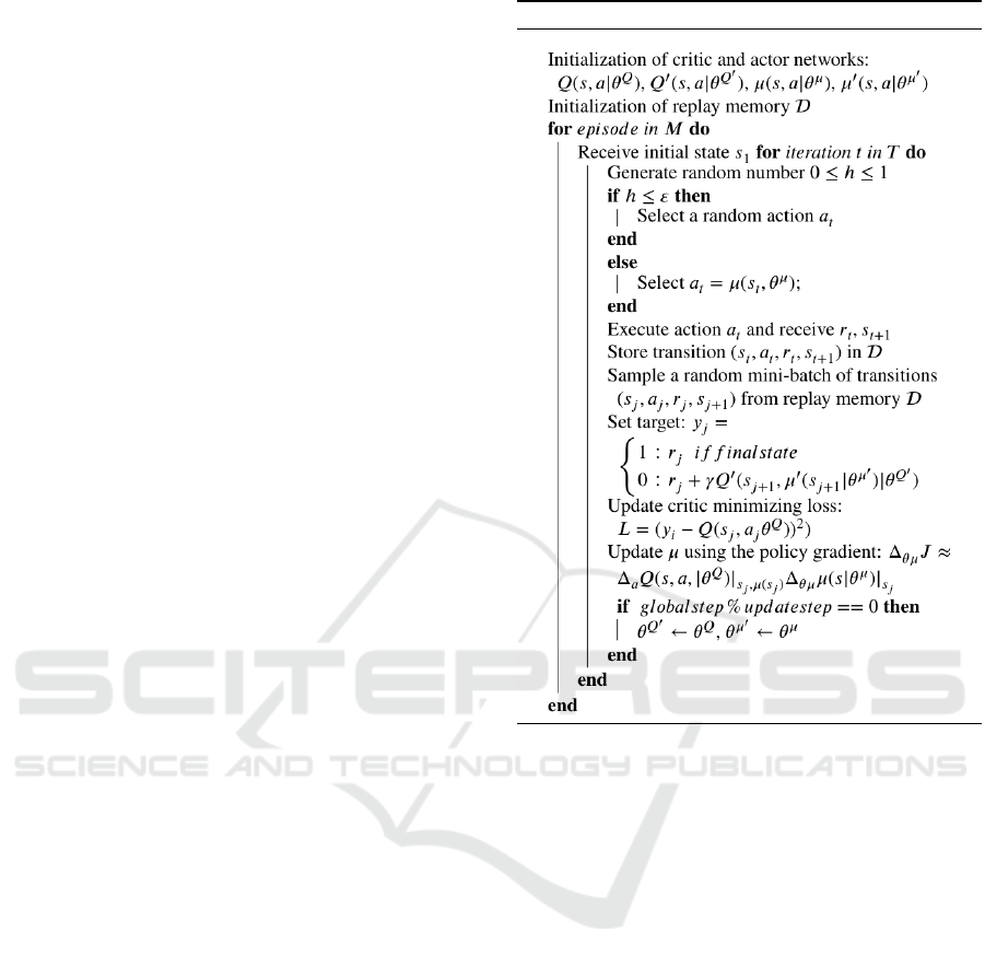
Algorithm 1: DDPG algorithm.
lects an action a
t
∈ A and performs it in the environ-
ment, which gives back a new state s
t+1
∈ S and a
reward r
t+1
, sequentially at each time-step t. The en-
vironment may also be stochastic. A and S are the
space of the actions and the space of the states, re-
spectively. The reward r
t
is the feedback signal at the
basis of the learning process from raw data, hence be-
ing higher for ”better” actions and lower for ”worse”
ones. The agent chooses an action by following a pol-
icy π that maps states to actions. A sequence with
shape s
0
,a
0
,r
1
,s
1
,a
1
,...,s
i
,a
i
,r
i+1
,s
i+1
is then gen-
erated, which can be seen as many transitions one af-
ter another. The training phase aims at making the
agent learn to maximize the return G, which is usu-
ally the discounted sum of future rewards, expressed
as
G =
∑
k=0
γ
k
R
t+k+1
(1)
The term γ is called discount factor and it regulates
the importance of rewards along the episode. It can
assume values between 0 (only the immediate reward
is important) and 1 (all future rewards are equally im-
portant). The agent is typically characterized by a pol-
icy π(a|s) which maps states to actions. A policy can
be stochastic, e.g. can give the probability of an ac-
Indoor Point-to-Point Navigation with Deep Reinforcement Learning and Ultra-Wideband
39

tion a to be taken when in state s, or deterministic,
hence giving the action directly and in this case is of-
ten denoted by µ.
Since the aim of an agent is to maximise G, it is
useful to define the expected return when an action a
t
is taken from a state s
t
and then a policy π is followed.
This is expressed by the action-value function:
Q
π
(s
t
,a
t
) = E
r
i≥t
,s
i>t
∼E,a
i>t
∼π
[R
t
| s
t
,a
t
] (2)
In many RL approaches the Bellman equation is
used:
Q
π
(s
t
,a
t
) = E
r
t
,s
t+1
∼E
[r(s
t
,a
t
)
+ γE
a
t+1
∼π
[Q
π
(s
t+1
,a
t+1
)]]
(3)
which, under target deterministic policy becomes:
Q
µ
(s
t
,a
t
) = E
r
t
,s
t+1
∼E
[r(s
t
,a
t
)
+ γ[Q
µ
(s
t+1
,a
t+1
)]]
(4)
This relationship is used to learn Q
µ
off policy,
that means that the exploited transition can also be
generated by using another stochastic behavioural
policy β. This approach can be referred to as Q-
learning. Considering a finite action space, once the
Q function is known, it is sufficient to choose the ac-
tion that maximizes the expected returns. This is also
called greedy policy:
µ(s) = argmax
a
Q(s,a) (5)
If we consider to approximate the action-value
function using a function approximator, whose pa-
rameters can be denoted as θ
Q
, the optimization can
be performed by minimizing the loss, which can be
expressed as:
L(θ
Q
) = E
s
t
∼ρ
β
,a
t
∼β,r
t
∼E
[(Q(s
t
,a
t
| θ
Q
) − y
t
)
2
] (6)
where:
y
t
= r(s
t
,a
t
) + γQ(s
t+1
,µ(s
t+1
| θ
Q
)) (7)
and ρ denotes the discounted state visitation distribu-
tion for a policy β. This procedure was recently used
along with two new feature: a replay buffer and a tar-
get network for obtaining the target y
t
(Mnih et al.,
2013)(Mnih et al., 2015).
2.2 Deep Deterministic Policy Gradient
The above seen Q-learning-related procedure cannot
be directly applied to a problem with a continuous ac-
tion space. So, we implement a version of the deep
deterministic policy gradient (DDPG) algorithm (Lil-
licrap et al., 2015) that uses an actor-critic approach to
overcome the limitations of discrete actions. Consid-
ering to be using function approximators, actor and
Figure 1: Scheme of used lidar measurements. Lower val-
ues of distance are considered more significant for obstacle
detection.
critic can be denoted respectively as µ(s | θ
µ
) and
Q(s,a | θ
Q
). The critic function is learned as done
in Q-learning, hence using the Bellman equation and
exploiting the same loss. The actor function instead
is updated by exploiting the knowledge of the pol-
icy gradient (Silver et al., 2014). Considering a start-
ing distribution J = E
r
i
,s
i
∼E,a
i
∼π
[R
1
] and applying the
chain rule to the expected return with respect to the
parameters of the actor, the policy gradient can be ob-
tained:
∆
θµ
J ≈ E
s
t
∼ρ
β
[∆
θµ
Q(s,a | θ
Q
) |
s=s
t
,a=µ(s
t
|θ
µ
)
]
= E
s
t
∼ρ
β
[∆
a
Q(s,a | θ
Q
) |
s=s
t
,a=µ(s
t
)
· ∆
θ
µ
µ(s | θ
µ
) |
s=s
t
]
(8)
The full pseudo-code is shown in Alg. 1. We
hardly update the target networks periodically instead
of performing a continuous soft update. Moreover, we
tackle the exploration-exploitation dilemma by main-
taining an ε probability to perform a random action
rather than following the policy µ. The value of ep-
silon decays during the training as:
ε = max(ε
0
ε
episode
d
,ε
min
) (9)
where ε
d
is the decay parameter.
2.3 Point-to-Point Agent Training
In this work, we deal with continuous domains, hold-
ing A ∈ R
N
(continuous control) and S ∈ R
M
(con-
tinuous state space), with N and M dimensions of ac-
tion and observation spaces. Concerning the latter,
the observation is the representation that the agent has
of the current state. In our case, the observation is a
vector with 62 elements. It is made of 60 1-D mea-
surements of the lidar, and distance and angle with
respect to the goal. During the simulation phase, we
use odometry data and magnetometer measurements
ICAART 2021 - 13th International Conference on Agents and Artificial Intelligence
40

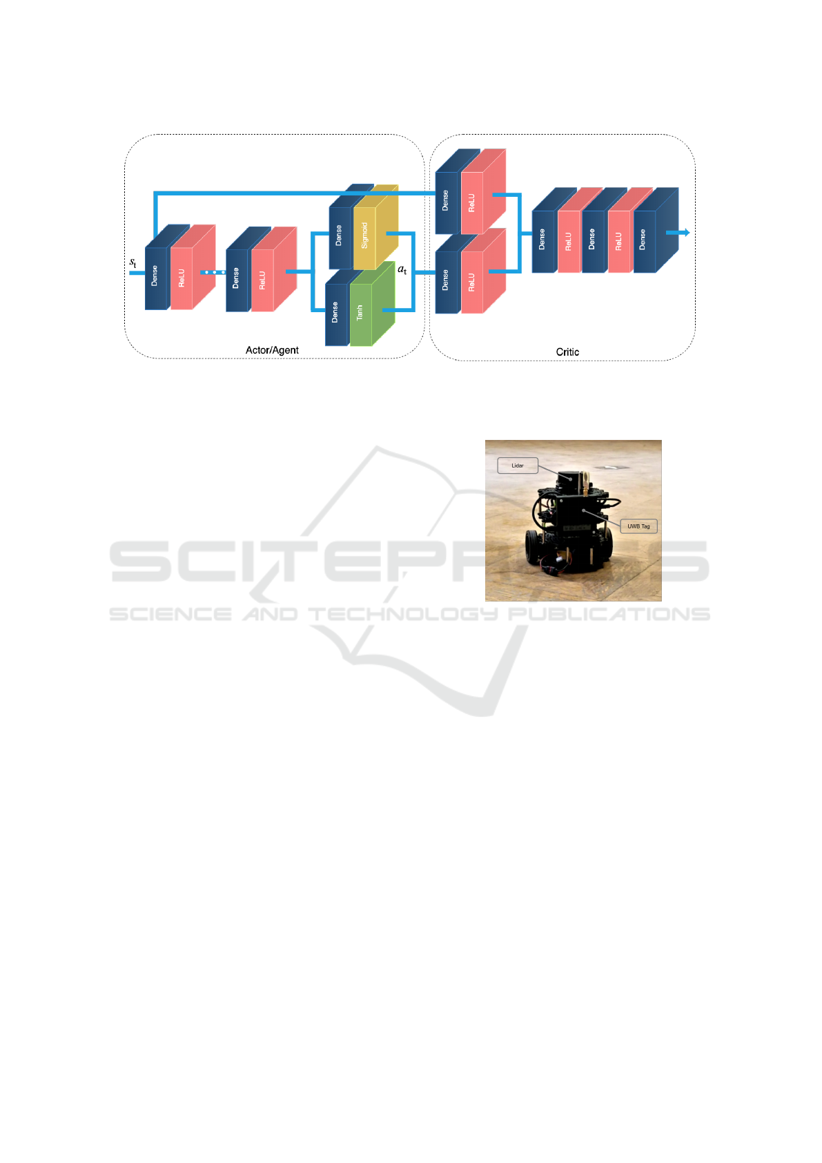
Figure 2: Graphical representation of the actor/critic architecture. During the training procedure, the actor processes the
observations of the robot s
t
with a cascade of fully connected layers producing distinct actions a
t
for the angular and linear
velocity. Subsequently, the critic network takes as input both s
t
and a
t
generating the corresponding Q value estimation. After
the training procedure, the policy learnt by the agent in simulation is exploited by the robot to navigate from point-to-point.
to compute and provide the previously mentioned dis-
tance and angle. This clearly demonstrates the robust-
ness of the trained agent, which is able to generalize
to the real scenario even without explicitly modelling
UWB localization signals during the training process.
The 1-D 60 measurements are not equally spaced. In-
stead, the whole 2π circle is split into 60 sectors, and
the minimum non-outliers are taken, to guarantee the
knowledge of nearer obstacles, as shown in Fig. 1.
The action instead is a 2-D vector, containing the
angular and the linear velocity of the robot:
• Linear velocity: the sigmoid activation function
guarantees a value between 0 and 1 since we
want the robot to only have non-negative values
of speed;
• Angular velocity: the hyperbolic tangent activa-
tion function constraints the output between −1
and 1.
According to the target network technique, we use
four networks: actor network, critic network and their
target twins, with the same architectures represented
in Fig. 2. The networks are mainly constituted by
fully connected layers with ReLU activation func-
tions, except for the final ones. The first three layers
of the actor have respectively 512, 256 and 256 neu-
rons. The critic first two hidden layers have respec-
tively 256 (state side) and 64 (action side) units. The
following hidden layers have 256 and 128 neurons se-
quentially. The last layer of the critic is a single out-
put FC with linear activation function to provide the
Q value.
Figure 3: The robotic platform used for the experimen-
tation: a Robotis TurtleBot3 Burger with a Decawave
EVB1000 Ultra-wideband tag.
3 EXPERIMENTAL DISCUSSION
AND RESULTS
In this section, we present the hardware and software
setup used during the experimentation phase. We pro-
vide a full description of the training phase of the RL
agent, with a detailed list of all the selected hyperpa-
rameters. Finally, we describe the different tests per-
formed and we present a quantitative evaluation of the
proposed local planner.
3.1 Hardware and Robotic Platform
The training of the RL agent is performed using a
workstation with an Intel Core i7 9700k CPU, along
with 64 GB of RAM. It takes around 24 hours to com-
plete. Concerning the robotic platform, we select the
Indoor Point-to-Point Navigation with Deep Reinforcement Learning and Ultra-Wideband
41

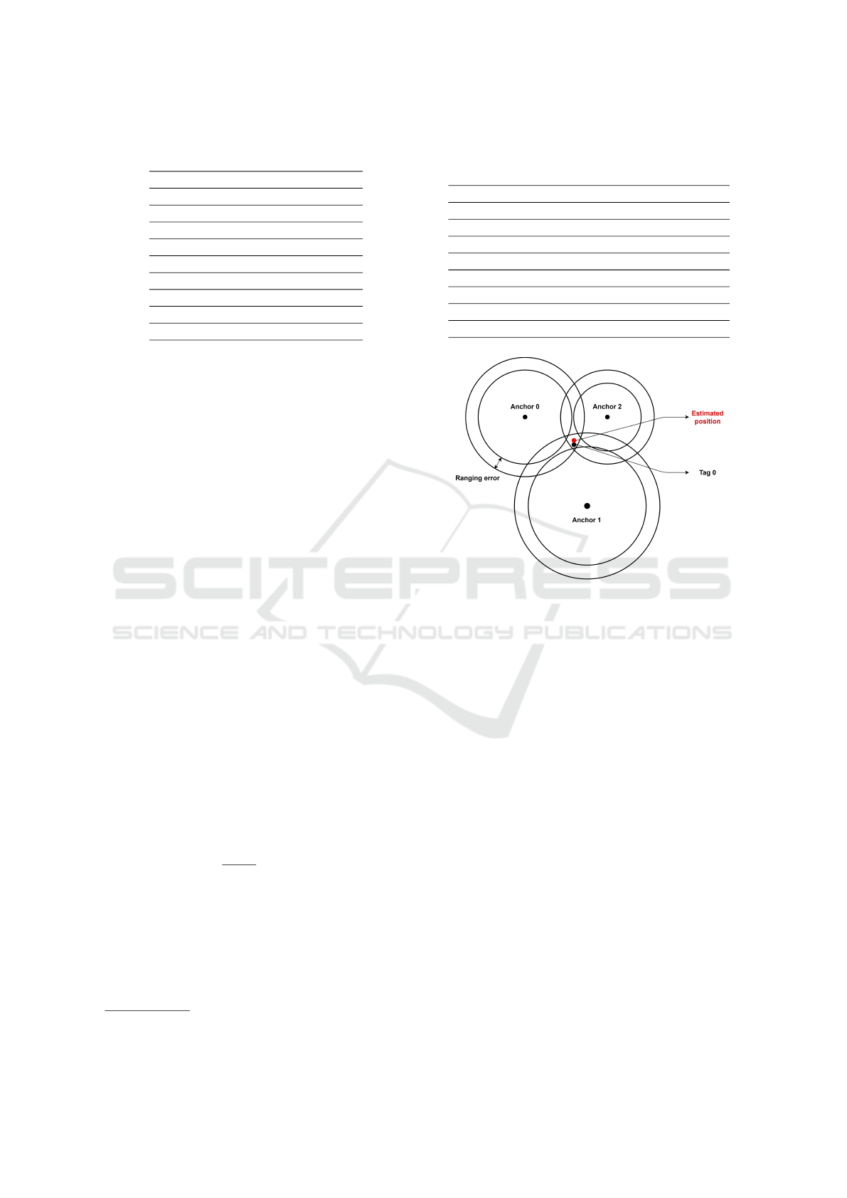
Table 1: Adopted hyperparameters in simulation during the
point-to-point agent training.
Hyper-parameters
starting epsilon 1
minimum epsilon 0.05
epsilon decay 0.998
learning rate 0.00025
discount factor 0.99
sample size 64
batch size 64
target network update 2000
deque memory maxlen 1000000
Robotis TurtleBot3 Burger model
1
, which is a low-
cost, ROS-oriented (Robot Operating System) solu-
tion. An accurate model is also provided for Gazebo
simulations. The Turtelbot3 Burger model we use is
equipped with a Raspberry Pi 3 B+. Concerning the
Ultra-wideband hardware, we use a TREK1000 eval-
uation kit by Decawave to provide the agent with the
localization data that in simulation are obtained via
odometry and magnetometer measurements. Fig. 3
shows the complete robotic platform used during the
experimentation.
3.2 RL Agent Training
The training is performed simulating both agent and
environment on Gazebo. The robot is controlled by
the actor network presented in the methodology. The
training is performed in episodes, that means the robot
is re-spawned in the same starting point. The objec-
tive for each episode is to reach a randomly spawned
goal and the reward that is given to the agent depends
on it. We use the following equation to provide re-
ward values:
R =





+1000, if goal is reached
−200, if collision occurs
3 · h
R
· 10 ·|∆d|, else,
(10)
where ∆d is the difference between distance at current
and previous instants of time, and:
h
R
= −

ω
t−1
·
1
1.2 · f
− heading

2
+ 1 (11)
is the heading reward. ω is the angular speed, while
f is the control frequency. The third part of the equa-
tion gives a positive reward when the robot is getting
closer to the goal (|∆d| contribute). Moreover, this
value is higher if it is directly pointing it (h
R
con-
tribute). The values of the hyperparameters used in
the training phase are shown in Tab. 1. The target
1
http://www.robotis.us/turtlebot-3/
Table 2: Selected settings of the robot and of the simulated
environment during the training of the deep reinforcement
learning agent.
Robot settings
lidar points 60
ctrl period 0.33
maximum angular speed 1rad/s
maximum linear speed 0.2m/s
Simulation settings
time step 0.0035s
max update rate 2000s
−
1
timeout 250s (in sim. time)
Figure 4: Estimation of the position in the x-y plan using
error affected ranging measurements.
network update sets how often the target networks are
hardly updated, in terms of steps. The same value of
learning rate is used for both actor and critic, equal to
0.00025. The discount factor is set to a value of 0.99,
as for the epsilon decay. Tab. 2 presents the environ-
ment and the robot settings used in simulation.
3.3 Ultra-Wideband Settings
In our experimental setup, we use UWB as the only
positioning method, do its robustness against the
noise in the localization measurements. The real-
time locating system (RTLS) is composed of 5 De-
cawave EVB1000 boards: 4 placed in fixed positions
(anchors) at the corners of the experimental area and
one mounted on the robotic platform. The EVB1000
boards are set to communicate using channel 2 (cen-
tral frequency 3.993 GHz) with a data rate of 6.8
Mbps, a preamble length of 128 symbols and a po-
sitioning update rate of 10 Hz. We mount the four
anchors on four tripods at slightly different heights,
with maximum height set at less than 2 meters. The
position of the anchors along the vertical axis strongly
affects the precision of the localization in the hor-
ICAART 2021 - 13th International Conference on Agents and Artificial Intelligence
42

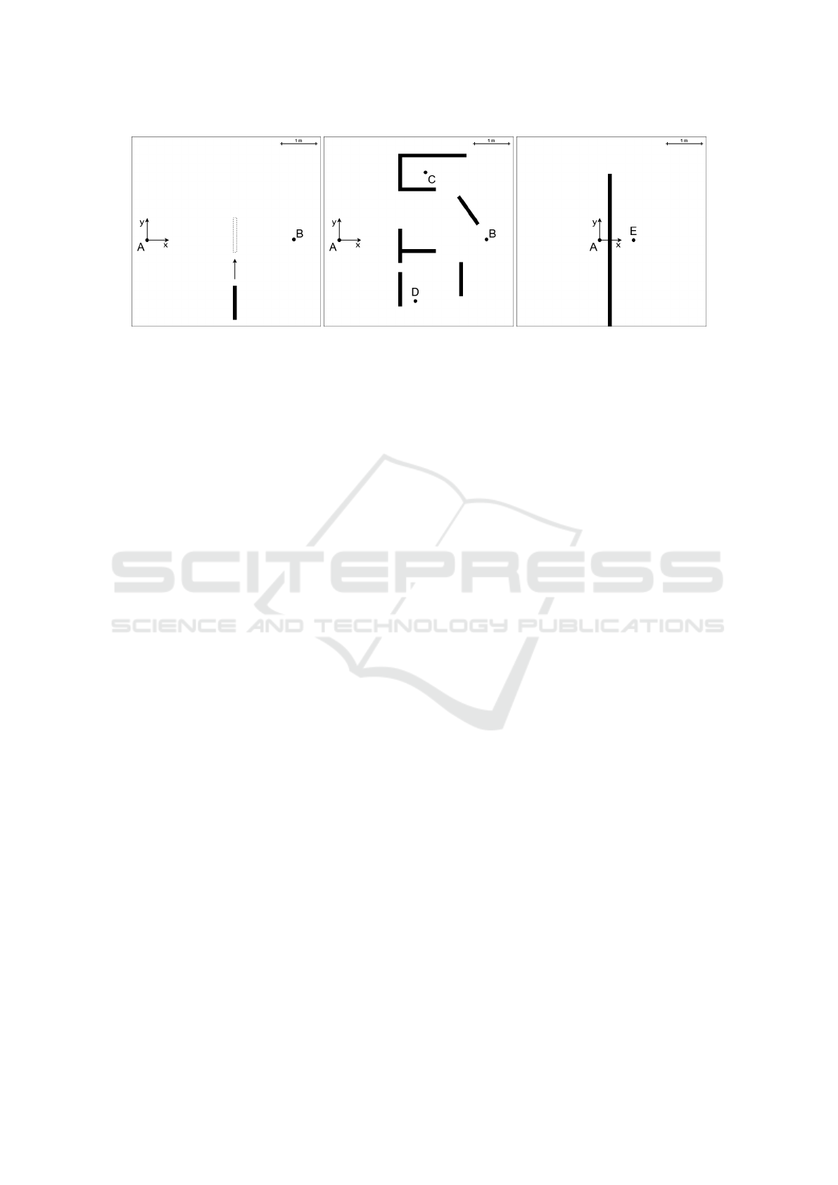
(a) Path: AB. (b) Path: ABCD. (c) Path: AE.
Figure 5: Scenarios used in the first set of tests for the local planner evaluation. Points positions: A(0, 0) m, B(4.35,0.02) m,
C(2.55, 2) m, D(2.25, −1.8) m, E(1, 0) m.
izontal (x-y) plan, increasing the height is possible
to achieve better performances. Moreover, the robot
(target) is able to move outside the area defined by
the fixed devices, and this is a critical situation for
the computation of the position. The raw ranging
data are smoothed using a simple linear Kalman fil-
ter. The measurement noise covariance, computed in
previous experiments, is set to σ
2
m
= 6.67 ∗ 10
−4
and
the process noise covariance (σ
2
p
= 10
−4
) is chosen
to obtain the desired behavior from the filter. Finally,
the position of the robot is computed as the intersec-
tion of the four spheres centered in the anchors’ po-
sitions with a radius equal to the corresponding rang-
ing measurements, as schematically shown in Fig. 4.
This is a typical nonlinear estimation problem that we
solve using the Gauss-Newton nonlinear least-squares
method, which is a well-suited algorithm for range-
based position estimation, as discussed in (Yan et al.,
2008). At each sampling step, the new position is esti-
mated starting the iteration from the last known point.
3.4 Experimental Settings
To prove the robustness and the reliability of the pro-
posed system, we perform several experimentations
that can be grouped into two test sets. In the first,
we compare our system with a classical one based on
the well-known Dynamic Window Approach (DWA)
(Fox et al., 1997) in different scenarios to prove that
our local planner achieves better performances, with
lower computational effort. In the second set of tests,
we focus on the robustness of the system to UWB
localization noise, and we compare it to the perfor-
mance obtained by humans put in the same testing
conditions of the RL agent. The achieved results
thoroughly show how the proposed system can rep-
resent a reliable and efficient local planner to enable
autonomous navigation in unknown and unstructured
environments.
In all the following tests, we fix the reference
frame on the initial position of the robot and measure
the positions with a Leica AT403 Laser Tracker. The
main metric for navigation performance is the suc-
cess rate. Each experiment is considered successful
if the robot is able to get within 20 cm to the target
position without getting stuck. Since the robot can
theoretically reach the goal also with random wander-
ing, we consider a maximum time t
max
. If the robot
is unable to reach the target position within this time
interval, the test is considered failed. Considering the
maximum linear speed of 0.22 m s
−1
of the Turtlebot3
Burger and an average path length of 5.5 m over all
the experiments, we consider 180 s as a reasonable
value for t
max
. Moreover, we consider the mean total
time t
mean
as a metric to understand how well the local
planner is able to find an optimal solution to the nav-
igation problem and RMS accelerations ˙v
RMS
,
˙
ω
RMS
as metrics for navigation smoothness. Finally, colli-
sions with static or moving obstacles are registered
for each test, since the ability to avoid them assumes
a vital relevance in robotic autonomous navigation.
3.5 Local Planner Quantitative
Evaluation
The first set of tests is aimed at comparing the pro-
posed local planner with the most used Dynamic Win-
dow Approach (DWA) (Fox et al., 1997). We use
the ROS implementation of this navigation algorithm,
based on the work of Brock et al. (Brock and Khatib,
1999). The two algorithms are compared with re-
peated tests in three different scenarios:
1. the robot has to navigate to the target point au-
tonomously and is suddenly interrupted by a mov-
ing obstacle;
Indoor Point-to-Point Navigation with Deep Reinforcement Learning and Ultra-Wideband
43

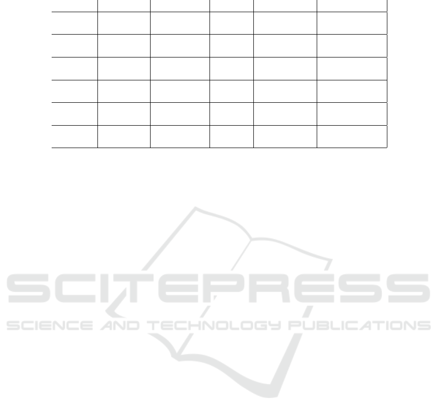
Table 3: Experimental results of the first set of tests: comparison with DWA (Fox et al., 1997) local planner.
Scenario Algorithm Success rate t
mean
[s] ˙v
RMS
[ms
−2
]
˙
ω
RMS
[rads
−2
]
S1
DWA 1 37 0.2277 1.1371
RL+UWB 1 33 0.1342 1.6382
S2
AB
DWA 0.80 48 0.3016 1.0022
RL+UWB 1 45 0.1535 2.6922
S2
BC
DWA 0.70 97 0.2866 1.6434
RL+UWB 0.91 65 0.1149 1.4719
S2
CD
DWA 0.50 129 0.2757 0.9180
RL+UWB 0.91 94 0.1050 1.5483
S2
ABCD
DWA 0.50 261 0.2880 1.1879
RL+UWB 0.91 223 0.1225 1.7528
S3
DWA 1 48 0.1920 1.1390
RL+UWB 1 31 0.1047 1.4132
2. the robot has to navigate to three waypoints in a
certain order inside a fairly complex environment;
3. the robot has to reach a goal located behind a wall,
with single opening quite far from the goal.
Fig. 5 shows a visual presentation of the first tests set
scenarios. The first one is particularly useful to eval-
uate the obstacle avoidance performance of the algo-
rithm and its ability to react to a sudden change in
the navigation environment, by following a new safer
path to reach the target. In this case, the moving ob-
stacle consists in a panel put in front of the robot while
it is navigating towards the target. The second sce-
nario shows the ability to solve subsequent point-to-
point tasks in a quite complex and unstructured envi-
ronment. The robot starts in point A and has to nav-
igate segments AB, BC, CD, subsequently. We eval-
uate performances both on the single point-to-point
tasks and on the whole path ABCD. Finally, the last
scenario is relevant to judge the ability of the algo-
rithm to adopt local sub-optimal actions that make the
robot actually increase the distance from the target, in
order to be subsequently able to reach the final goal.
In this sense, this kind of situation is useful to evalu-
ate whether the robot is able to escape local minima.
We perform a total of 30 tests for both the algo-
rithms in the three different scenarios. Tab. 3 summa-
rizes the experimentation. In general, our approach
has a higher success rate and requires, on average, less
time to reach the target. It gets lower linear acceler-
ations, but higher angular ones, resulting in a lower
smoothness on the angular control. The second sce-
nario appears to be the toughest one, in particular in
its third task CD, where the DWA success rate drops
to 0.5. In all these tests, we register no collisions with
both the algorithms. However, the main advantage of
the proposed local planner is its computational effort.
We achieve up to 400 Hz control frequency the pro-
posed RL planner. On the other hand, since the DWA
is an optimization algorithm, on the same machine it
ranges between 0.5 Hz and 5 Hz. This dramatic im-
provement in computational efficiency allows for the
proposed local planner to be completely run in an em-
bedded system on the robot itself, without the need of
a powerful machine as classic algorithms as DWA do.
We deploy the RL agent on a Raspberry Pi3 B+ em-
bedded computer, and we are able to achieve a real-
time control at about 30 Hz.
3.6 Noise Robustness and Human
Comparison
The second set of tests is aimed at comparing the
proposed algorithm with human performance, as well
as demonstrate how the RL+UWB system is highly
robust against localization noise. In literature, RL
agents are frequently compared to human agents to
prove their control performance in complex tasks
(Mnih et al., 2015; Silver et al., 2016; Mirowski et al.,
2016; Silver et al., 2018). We perform such compari-
son by putting several people in the same experimen-
tal conditions of the RL agent. Human testers are kept
in a different room with respect to the experimental
environment and can see in real-time the robot posi-
tion, the goal and the 1-D lidar range measurements,
that are exactly the same information available to the
RL planner. Fig. 7 presents the interface shown to hu-
man testers during the experimentation. Both humans
and RL agent are tested in the following scenarios,
shown in Fig. 6:
1. the robot has to navigate to the target point au-
tonomously and is suddenly interrupted by a per-
son;
2. the robot has to pass through a small opening par-
tially occluded by a moving obstacle;
3. the robot has to navigate to three waypoints in a
certain order inside a fairly complex environment;
ICAART 2021 - 13th International Conference on Agents and Artificial Intelligence
44

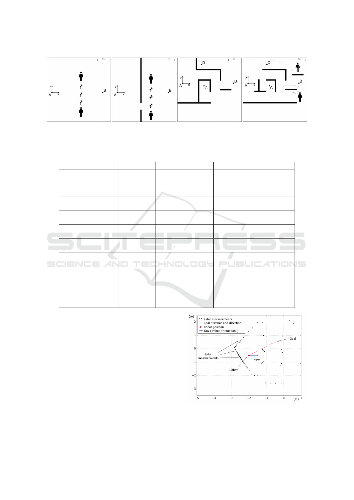
(a) Path: AB. (b) Path: AB. (c) Path: ABCD.
(d) Path: ACBD.
Figure 6: Scenarios used in the second set of tests for the comparison with human control. Points positions: A(0, 0) m,
B(4.45,0.02) m, C(1.86,−0.21) m, D(1.65, 1.65) m.
Table 4: Experimental results of the second set of tests: comparison with human control.
Scenario Agent Success rate Collisions t
mean
[s] ˙v
RMS
[ms
−2
]
˙
ω
RMS
[rads
−2
]
S1
Human 1 0 30 0.3574 2.0783
RL+UWB 1 0 29 0.3557 3.8413
S2
Human 1 0.25 42 0.3382 2.0012
RL+UWB 1 0 50 0.3333 4.5058
S3
AB
Human 1 0.25 38 1.7703 2.1109
RL+UWB 1 0 39 0.3513 4.1098
S3
BC
Human 1 0.50 36 0.3643 2.0638
RL+UWB 1 0 29 0.3495 4.1354
S3
CD
Human 0.75 0.25 97 0.3691 2.1878
RL+UWB 0 0 - - -
S3
ABCD
Human 0.75 1 161 0.3696 2.1490
RL+UWB 0 0 - - -
S4
AC
Human 1 0 49 0.3227 2.1171
RL+UWB 1 0 49 0.3230 4.5523
S4
CB
Human 1 0.25 40 0.3224 2.3882
RL+UWB 1 0 28 0.3393 4.4387
S4
BD
Human 1 0 49 0.3420 2.1848
RL+UWB 1 0 25 0.3280 4.3618
S4
ACBD
Human 1 0.25 137 0.3290 2.2301
RL+UWB 1 0 102 0.3301 4.4509
4. the robot has to navigate to three waypoints in
a certain order inside a fairly complex environ-
ment with both static and moving obstacles (peo-
ple wandering in the scenario).
In all these tests, Gaussian noise is superimposed to
UWB measurements in order to evaluate the robust-
ness of the system to localization errors. Higher un-
certainty in the UWB positioning is also caused by
the presence of people in the environments (scenarios
1, 2, 4) who obstruct the anchors and cause the NLOS
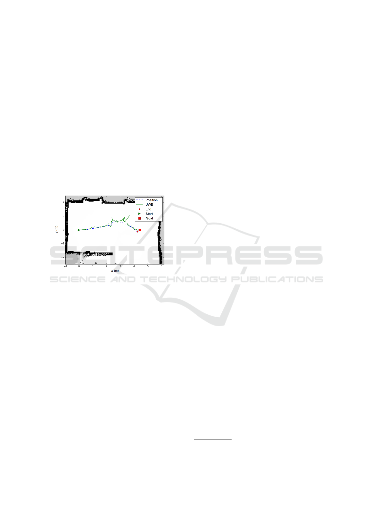
(non-line of sight) condition. Fig. 8 shows an exam-
ple of the trajectory followed by the robot in the first
scenario (path AB, interrupted by a sudden moving
person). The noisy signal of the UWB clearly gives
a high uncertainty on the position of the robot. How-
ever, the RL local planner is highly robust against lo-
calization errors and it is able to reach the goal.
Figure 7: Human interface during the second tests set.
Testers are allowed to see lidar measurements, robot pose
and goal distance and direction.
Indoor Point-to-Point Navigation with Deep Reinforcement Learning and Ultra-Wideband
45

Tab. 4 presents the results of the second set of
tests. In general, the RL+UWB appears to have
similar performances to human control, even in the
presence of localization noise. The proposed algo-
rithm appears to be particularly able in avoiding ob-
stacles, while humans result more subject to collisions
in complex environments. One interesting thing to
notice is that the RL+UWB is completely unable to
solve the CD task of scenario 3, when the robot is sur-
rounded by walls on three edges. It remains stuck,
repeating the same actions over and over. This behav-
ior can be explained by the absence of memory in this
kind of planners, that makes them unable to escape
from too narrow local minima. Humans are able to
analyze subsequent states and can understand how the
environment is actually disposed, while the RL agent
simply reacts to the current state and cannot build an
environment map.
Figure 8: Trajectory followed in a test in the first scenario
(path AB, interrupted by a sudden moving person). The
UWB added noise is clearly visible and shows how the pro-
posed local planner is highly robust against positioning er-
rors.
4 CONCLUSION
In this paper, we proposed a novel indoor local mo-
tion planner based on a strict synergy between an
autonomous agent trained with deep reinforcement
learning and ultra-wideband localization technology.
Indoor autonomous navigation is a challenging task,
and localization techniques can generate noisy and
unreliable signals. Moreover, due to the high com-
plexity of typical environments, hand-tuned classical
methodologies are highly prone to failure and require
access to a large number of computational resources.
The extensive experimentation and evaluations of our
research proved that our low-cost and power-efficient
solution has comparable performance with classical
methodologies and is robust to noise and scalable to
dynamic and unstructured environments.
ACKNOWLEDGEMENTS
This work has been developed with the contribution of
the Politecnico di Torino Interdepartmental Centre for
Service Robotics PIC4SeR
2
and SmartData@Polito
3
.
This work is partially supported by the Italian govern-
ment via the NG-UWB project (MIUR PRIN 2017).
REFERENCES
Aghi, D., Mazzia, V., and Chiaberge, M. (2020). Local mo-
tion planner for autonomous navigation in vineyards
with a rgb-d camera-based algorithm and deep learn-
ing synergy. Machines, 8(2):27.
Barraquand, J. and Latombe, J.-C. (1991). Robot mo-
tion planning: A distributed representation approach.
The International Journal of Robotics Research,
10(6):628–649.
Brock, O. and Khatib, O. (1999). High-speed navigation us-
ing the global dynamic window approach. In Proceed-
ings 1999 IEEE International Conference on Robotics
and Automation (Cat. No. 99CH36288C), volume 1,
pages 341–346. IEEE.
Cadena, C., Carlone, L., Carrillo, H., Latif, Y., Scaramuzza,
D., Neira, J., Reid, I., and Leonard, J. J. (2016). Past,
present, and future of simultaneous localization and
mapping: Toward the robust-perception age. IEEE
Transactions on robotics, 32(6):1309–1332.
Chen, C., Seff, A., Kornhauser, A., and Xiao, J. (2015).
Deepdriving: Learning affordance for direct percep-
tion in autonomous driving. In Proceedings of the
IEEE International Conference on Computer Vision,
pages 2722–2730.
Chiang, H.-T. L., Faust, A., Fiser, M., and Francis, A.
(2019). Learning navigation behaviors end-to-end
with autorl. IEEE Robotics and Automation Letters,
4(2):2007–2014.
Fox, D., Burgard, W., and Thrun, S. (1997). The dy-
namic window approach to collision avoidance. IEEE
Robotics & Automation Magazine, 4(1):23–33.
Khaliq, A., Mazzia, V., and Chiaberge, M. (2019). Refining
satellite imagery by using uav imagery for vineyard
environment: A cnn based approach. In 2019 IEEE
International Workshop on Metrology for Agriculture
and Forestry (MetroAgriFor), pages 25–29. IEEE.
Lillicrap, T. P., Hunt, J. J., Pritzel, A., Heess, N., Erez, T.,
Tassa, Y., Silver, D., and Wierstra, D. (2015). Contin-
uous control with deep reinforcement learning.
Magnago, V., Corbal
´
an, P., Picco, G., Palopoli, L.,
and Fontanelli, D. (2019). Robot localization
via odometry-assisted ultra-wideband ranging with
stochastic guarantees. In Proc. IEEE/RSJ Int. Conf.
Intell. Robots Syst.(IROS), pages 1–7.
Mazzia, V., Khaliq, A., and Chiaberge, M. (2020). Improve-
ment in land cover and crop classification based on
2
https://pic4ser.polito.it
3
https://smartdata.polito.it
ICAART 2021 - 13th International Conference on Agents and Artificial Intelligence
46

temporal features learning from sentinel-2 data using
recurrent-convolutional neural network (r-cnn). Ap-
plied Sciences, 10(1):238.
Mirowski, P., Pascanu, R., Viola, F., Soyer, H., Ballard,
A. J., Banino, A., Denil, M., Goroshin, R., Sifre,
L., Kavukcuoglu, K., et al. (2016). Learning to
navigate in complex environments. arXiv preprint
arXiv:1611.03673.
Mnih, V., Kavukcuoglu, K., Silver, D., Graves, A.,
Antonoglou, I., Wierstra, D., and Riedmiller, M.
(2013). Playing atari with deep reinforcement learn-
ing. arXiv preprint arXiv:1312.5602.
Mnih, V., Kavukcuoglu, K., Silver, D., Rusu, A. A., Veness,
J., Bellemare, M. G., Graves, A., Riedmiller, M., Fid-
jeland, A. K., Ostrovski, G., et al. (2015). Human-
level control through deep reinforcement learning.
Nature, 518(7540):529.
Mocanu, E., Mocanu, D. C., Nguyen, P. H., Liotta, A., Web-
ber, M. E., Gibescu, M., and Slootweg, J. G. (2018).
On-line building energy optimization using deep re-
inforcement learning. IEEE Transactions on Smart
Grid.
Mohanan, M. and Salgoankar, A. (2018). A survey of
robotic motion planning in dynamic environments.
Robotics and Autonomous Systems, 100:171–185.
Rigelsford, J. (2004). Introduction to autonomous mobile
robots. Industrial Robot: An International Journal.
Salvetti, F., Mazzia, V., Khaliq, A., and Chiaberge, M.
(2020). Multi-image super resolution of remotely
sensed images using residual attention deep neural
networks. Remote Sensing, 12(14):2207.
Silver, D., Huang, A., Maddison, C. J., Guez, A., Sifre, L.,
Van Den Driessche, G., Schrittwieser, J., Antonoglou,
I., Panneershelvam, V., Lanctot, M., et al. (2016).
Mastering the game of go with deep neural networks
and tree search. nature, 529(7587):484.
Silver, D., Hubert, T., Schrittwieser, J., Antonoglou, I., Lai,
M., Guez, A., Lanctot, M., Sifre, L., Kumaran, D.,
Graepel, T., et al. (2018). A general reinforcement
learning algorithm that masters chess, shogi, and go
through self-play. Science, 362(6419):1140–1144.
Silver, D., Lever, G., Heess, N., Degris, T., Wierstra, D., and
Riedmiller, M. (2014). Deterministic policy gradient
algorithms. In Proceedings of the 31st International
Conference on International Conference on Machine
Learning - Volume 32, ICML’14, page I–387–I–395.
JMLR.org.
Tamar, A., Wu, Y., Thomas, G., Levine, S., and Abbeel,
P. (2016). Value iteration networks. In Advances in
Neural Information Processing Systems, pages 2154–
2162.
Yan, J., Tiberius, C., Bellusci, G., and Janssen, G. (2008).
Feasibility of gauss-newton method for indoor posi-
tioning. In 2008 IEEE/ION Position, Location and
Navigation Symposium, pages 660–670.
Zafari, F., Gkelias, A., and Leung, K. K. (2019). A survey
of indoor localization systems and technologies. IEEE
Communications Surveys & Tutorials.
Zhu, Y., Mottaghi, R., Kolve, E., Lim, J. J., Gupta, A., Fei-
Fei, L., and Farhadi, A. (2017). Target-driven visual
navigation in indoor scenes using deep reinforcement
learning. In 2017 IEEE international conference on
robotics and automation (ICRA), pages 3357–3364.
IEEE.
Indoor Point-to-Point Navigation with Deep Reinforcement Learning and Ultra-Wideband
47