A History-based Framework for Online Continuous Action Ensembles

in Deep Reinforcement Learning

Renata Garcia Oliveira

and Wouter Caarls

Pontiﬁcal Catholic University of Rio de Janeiro, Rio de Janeiro RJ 38097, Brazil

Keywords:

Reinforcement Learning, Deep Reinforcement Learning, Continuous Ensemble Action, Ensemble

Algorithms, Hyperparameter Optimization.

Abstract:

This work seeks optimized techniques of action ensemble deep reinforcement learning to decrease the hyper-

parameter tuning effort as well as improve performance and robustness, while avoiding parallel environments

to make the system applicable to real-world robotic applications. The approach is a history-based frame-

work where different DDPG policies are trained online. The framework’s contributions lie in maintaining a

temporal moving average of policy scores, and selecting the actions of the best scoring policies using a single

environment. To measure the sensitivity of the ensemble algorithm to the hyperparameter settings, groups were

created that mix different amounts of good and bad DDPG parameterizations. The bipedal robot half cheetah

environment validated the framework’s best strategy surpassing the baseline by 45%, even with not all good

hyperparameters. It presented overall lower variance and superior results with mostly bad parameterization.

1 INTRODUCTION

Reinforcement learning (RL) (Sutton and Barto,

2018) is based on a mathematical framework known

as a Markov Decision Process (MDP). It is widely

used for controlling environments, maximizing a re-

ward signal for trial and error in order to achieve a

goal. Deep Deterministic Policy Gradient (DDPG) is

a model-free algorithm that can learn policies in high-

dimensional state space and continuous action space

(Lillicrap et al., 2016; Silver et al., 2014).

RL algorithms such as DDPG need ﬁne-tuning of

their hyperparameters to converge. The search for

best parameters can be performed by grid search. This

procedure is computationally expensive, hence there

are several hyperparameters optimization methods;

recent studies use bayesian optimization (Bertrand,

2019), bandit-based approach (Li et al., 2018), ge-

netic algorithm (Fernandez and Caarls, 2018) and se-

quential decision (Wistuba et al., 2015). Another

method for learning optimal parameters is population-

based training (PBT) (Jaderberg et al., 2017) and

CERL (Khadka et al., 2019), it uses multiple learn-

ers as a population to train neural networks inspired

by genetic algorithm, copying the best hyperparame-

https://orcid.org/0000-0001-8226-3178

https://orcid.org/0000-0001-9069-2378

ters across the population. Unlike these, population-

guided parallel policy search (Jung et al., 2020) opti-

mizes by using a soft manner to guide a better search.

The population based approaches consider multiple

environments.

As opposed to hyperparameter tuning for super-

vised learning, where the same data set can be re-used

over and over, RL demands new environment data ac-

quisition for each conﬁguration, since it is necessary

to run the control policy being optimized in the en-

vironment, which takes time. In addition, applying

this process in the real world takes much longer, and

risks damage to the robot (Tan et al., 2018). The goal

is to learn from a single environment combining an

ensemble of continuous actors while improving per-

formance and robustness.

Action ensembles in literature use pre-learned al-

gorithms. In discrete actions, ensemble algorithms

(Wiering and Van Hasselt, 2008) are combined in

a single agent using action probability aggregations,

among them the majority voting ensemble signiﬁ-

cantly outperforms others methods in ﬁnal perfor-

mance running in maze environments. For continuous

action, ensembles of neural networks (Hans and Ud-

luft, 2010) use Neural Fitted Q-Iteration and presents

advantages in majority voting action aggregation over

Q-averages aggregation in the pole balancing environ-

ment, being advisable to use different network topolo-

580

Oliveira, R. and Caarls, W.

A History-based Framework for Online Continuous Action Ensembles in Deep Reinforcement Learning.

DOI: 10.5220/0010199005800588

In Proceedings of the 13th International Conference on Agents and Artiﬁcial Intelligence (ICAART 2021) - Volume 2, pages 580-588

ISBN: 978-989-758-484-8

gies. Another study presents the data center and the

density based aggregations (Duell and Udluft, 2013),

the latter results in reliable policies in most experi-

ments with neural network-based RL in a gas turbine

simulation A recent study uses mean aggregation of

continuous action in a deep ensemble reinforcement

learning with multiple DDPG (Wu and Li, 2020) to

train autonomous vehicles in multiple environments.

As opposed to cited literature, we speciﬁcally tar-

get online learning policies in a single environment, to

make it possible the use in real system, in addition to

reducing the hyperparameter tuning effort. A History-

Based Framework is proposed to aggregate the con-

tinuous actions leading to a good result even if some

algorithms do not converge separately. The main con-

tribution resides in the use of a temporal moving av-

erage of policy scores and also in the online selection

of the best scoring policies.

This article is organized in 6 sections. Section 2

presents the background of DDPG and Ensemble Ac-

tions. Section 3 presents the History-Based Frame-

work to continuous action ensembles in DDPG. Sec-

tion 4 explains the planning and execution of the ex-

periments. Finally, sections 5 and 6 present the dis-

cussion and conclusion of the work.

2 BACKGROUND

DDPG. It is an actor-critic algorithm applicable in

continuous-action tasks with high dimensional state

spaces (Lillicrap et al., 2016). It is an approach based

on the Deterministic Policy Gradient (DPG) algo-

rithm (Silver et al., 2014). The critic Q(s, a) learns to

approximate a value function satisfying the Bellman

equation as in deep Q-learning (Mnih et al., 2014).

DDPG optimizes the critic by minimizing the loss

(Equation (1) and (2)), where the function approxi-

mator is parameterized by θ

and θ

, the former be-

longing to the training network and the latter referring

to the target network. s and a are the state and action

in a certain time step, r is the reward and s

represents

the next state. The loss function is

L(θ

) = E

(s,a,r,s

)



− Q(s, µ(s)|θ

)



(1)

where

= r

+ γQ(s

, µ(s

)|θ

) (2)

The Bellman error of the value function of the tar-

get policy is the performance objective, averaged over

the state distribution of the behaviour policy. The

policy is learned from a parameterized actor function

µ(s|θ

), which deterministically maps states to a spe-

ciﬁc action. Equation (3) presents the actor update,

which takes a step in the positive gradient criteria of

the critic with respect to the actor parameters. Ap-

plying the chain rule, J represents the expected return

over the start distribution and ρ

a different (stochas-

tic) behavior policy.

∇

J =

∼ρ



∇

Q(s, a|θ

s=s

,a=µ(s

)

∇

µ(s|θ

s=s

)



(3)

Taking advantage of off-policy data, experiments are

stored for use as a Replay Memory, inducing sam-

ple independence. The samples s, a, r, s

are generated

by exploring sequentially the environment and storing

them in the replay memory (R ). Every time step, a

minibatch is sampled uniformly from the replay mem-

ory, updating the actor and critic. This memory size is

chosen big enough to avoid overﬁtting (Liu and Zou,

2018).

Note that y

in Eq (2) depends on θ

, a target

network used to stabilize the network learning with

a time delay. This “soft” target update considers the

exponentially decaying average for actor and critic

networks parameters as in Equation (4). This tech-

nique stabilizes the problem of learning the action-

value function and brings the problem closer to the

case of supervised learning (Lillicrap et al., 2016).

0(t)

= τθ

(t−1)

+ (1 − τ)θ

0(t−1)

with τ ∈ [0, 1] (4)

The exploration in continuous action spaces is a chal-

lenge in RL. A noise N is added to sample the pol-

icy π = µ(s

|θ

) + N . The N uses the Ornstein-

Uhlenbeck process (Uhlenbeck and Ornstein, 1930)

to generate temporally correlated exploration for ex-

ploration efﬁciency in physical environments that

have momentum (N θ = 0.15 and N σ = 1). The

Ornstein-Uhlenbeck process models the velocity of a

Brownian particle with friction, which results in tem-

porally correlated values centered around zero (Lilli-

crap et al., 2016).

Ensemble Aggregation. These techniques below

form a base case in experiments. Figure 1 illustrates

the interaction.

• Density Based: is a way to extend majority voting

to continuous action spaces. It seeks the action

with the highest density (d

) in the space of actions

(Duell and Udluft, 2013).

The density d

is calculated for each action a

in the action ensemble of cardinality N using an

isotropic Gaussian density over its k dimensions,

where each action dimension is normalized to

[−1;1]. The distance parameter r is using value

A History-based Framework for Online Continuous Action Ensembles in Deep Reinforcement Learning

581

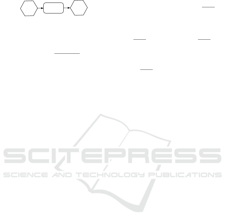
(1)

Ensemble

Aggregation

(A)

Action

Ensemble

(B)

Center

Action

Figure 1: Conventional Ensemble Aggregation Strategy.

0.025. After calculating all actions’ densities, the

action with the highest density value is chosen.

∑

j=1

−

∑

l=1

(

−a

)

(5)

• Data Center: in the ﬁrst step, the Euclidean dis-

tance is calculated for each action with respect

to the mean of the action ensemble. The action

with the longest distance is removed and the pro-

cedure is repeated until only two actions remain

(Duell and Udluft, 2013). Finally, the average of

the last two actions is the chosen action. This is a

parameter-free algorithm.

• Mean: this function returns the arithmetic mean of

the ensemble actions, or sum of all values divided

by the total number of values. If we are dealing

primarily with well-tuned hyperparameters algo-

rithms and up to 3 learners agent, this should lead

to a good ensemble action (Wu and Li, 2020).

3 HISTORY-BASED

FRAMEWORK

Ordinarily, ensemble aggregations consider pre-

learned policies, while this study aims to perform on-

line action aggregation. Assuming that policy perfor-

mance is time-correlated, the framework uses histor-

ical performance to make decisions. As such, poli-

cies with bad performance in the past can be dis-

carded from the aggregation. The Ensemble Frame-

work, presented in Figure 2, was created to select the

best ensemble action. In order to explore the best way

to deﬁne historical performance, the framework al-

lows different scoring functions. Before explaining

the framework step by step, it is important to high-

light its mechanisms.

Performance History Parameter. Although con-

sidering that the ensemble can make a better trade-off

between exploration and exploitation (Wiering and

Van Hasselt, 2008), it has been found empirically that

it can be difﬁcult for the ensemble aggregations to

maintain consistency when simply selecting the ac-

tion of the highest scoring algorithm in the ensem-

ble. Therefore, an exponentially weighted moving

average ﬁlter is applied, reducing the action chatter-

ing between the algorithms. For this, the scores vari-

able accumulates performance at each time step using

the historical learning rate α

= 0.01 (chosen empiri-

cally) as shown in Equation (6).

scores = α

· scores + (1 − α

) · scores (6)

Active Set Aggregation. It was created to take ad-

vantage of action ﬁltering that becomes possible due

to the performance history. The group is ranked ac-

cording to scores which allows ﬁltering the actions of

the best performing parametrizations. Thus, the best

actions compose a new action ensemble and a new ag-

gregation is performed to select the best action from

the active set.

3.1 Framework

This section presents the framework as a structure of

functions and intermediate data that allow applying

the exponential moving average ﬁlter, using various

techniques and evaluatons in order to ﬁnd the most ef-

ﬁcient among the environments. At the beginning of

Figure 2, the Framework seeks to score the ensemble

of actions — (A) Action Ensemble — by an aggrega-

tion strategy, thus the (1) Ensemble Aggregation uses

methods described in Section 2 to ﬁnd (B) Center Ac-

tion. This step is only necessary when the Squared

Euclidean Distance is used in the next function —

(2) Scoring. Otherwise, another scoring function that

does not require a center action is used.

The (A) and (B) data serve as input to (2) Scoring

which calculates a weighting of values, a score, for

each action — (C) Scores. The following methods

are speciﬁcally used or adapted for this scoring step:

Data Center Ranking, Density Raking and Squared

Euclidean Distance.

Data Center Ranking. The data center ranking

uses the concept of data center (Section 2). During the

process of selecting the center element, the one far-

thest from the center is selected to be removed. Data

Center Ranking returns the step at which the partic-

ular policy’s action was removed, where the smallest

value is the center itself.

Density Scores. The density of each action (d

) is

presented in Section 2. In Density Based Aggrega-

tion, the density information d

assigned to each ac-

tion is returned.

ICAART 2021 - 13th International Conference on Agents and Artiﬁcial Intelligence

582

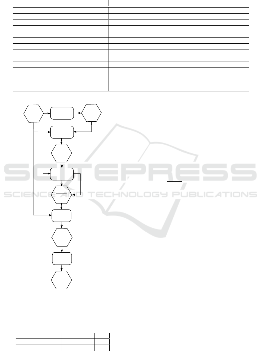
Table 1: Table with the hyperparameters’ description used to build each algorithm of the ensemble.

Hyperparameters Value Description

discount factor 0.98 or 0.99 Discount factor used in the Q-learning update.

reward scale 0.001, 0.1 or 1 Scaling factor applied to the environment’s rewards.

soft target update rate 0.01 Update rate of the target network weights.

target network 10 or 100 Steps number, or frequency, with which the target

update interval network parameters are updated.

learning rate 0.001 and 0.0001 Update rate used by AdamOptimizer.

replay steps 32 to 512 Number of minibatches used in a single step.

minibatch size 32 to 512 Number of transitions from the environment used in batch to

update the network.

layer size 50 to 400 Number of neurons in regular densely-connected NN layers

activation layer relu or softmax Output function of the hidden layers.

replay memory size 1000000 Size of the replay memory array that stores the agent’s

experiences in the environment.

observation steps 1000 Observation period to start replay memory using random policy.

(1)

Ensemble

Aggregation

(A)

Action

Ensemble

(2)

Scoring

(F)

Final

Action

(3)

Moving

Average

(4)

Percentile

Filtering

(D)

Scores

(5)

Active Set

Aggregation

(E)

Active Set

Actions

(C)

Scores

(B)

Center

Action

Figure 2: History-Based Framework for Ensemble Aggre-

gation.

Table 2: Composition of test conﬁgurations. The values

indicate how many parameterizations of each category were

included resulting in a group of 16 algorithms.

parametrizations good mid bad

best 12 8 4

worst 4 8 12

Squared Euclidean Distance. This is a well know

approach, very effective and widely used in the liter-

ature (Krislock and Wolkowicz, 2012). Equation (7)

presents the square of the difference between a policy

action and some aggregate action ¯a. ¯a can be cal-

culated using any of the ensemble aggregation tech-

niques described in Section 2.

∑

j=1

i j

− ¯a)

(7)

The (3) Moving Average uses the (C) Scores to up-

date the (D) Scores, history based variable, presented

in Equation (6). The function of the framework is the

(4) Percentile Filtering, where the speciﬁed percent-

age of the (A) Action Ensemble is selected based on

the order of scores to form the (E) Active Set Actions.

The idea is to use the scores’ history to ﬁlter the best

actions, safeguarding those policies that perform well

over time. Finally, the (F) Final Action is selected by

the (5) Active Set Aggregation. The aggregation used

here is Best, Data Center, Density Based and Mean.

The best aggregation selects the best action based on

the scores; in this conﬁguration ﬂow , the (4) Per-

centile Filtering function is not relevant.

The code used in the framework is available in

GRL (https://github.com/renata-garcia/grl).

4 EXPERIMENTS

In order to verify the efﬁciency of actor ensembles,

we used an approach testing three groups of good and

bad parametrizations with different algorithms. For

this, 32 DDPG agents with different hyperparame-

ters were individually tested. Table 1 presents the

hyperparameters values which were derived from the

DDPG presented in literature (Lillicrap et al., 2016).

A History-based Framework for Online Continuous Action Ensembles in Deep Reinforcement Learning

583

Note that, not necessarily good hyperparameters in

one environment will be good in the other. As such,

the classiﬁcation of a parameterization as either good

or bad depends on the environment.

Three groups were created and called good, mid

and bad. The groups were created to measure the

interference of bad hyperparameters on the methods.

The average end performance of 31 (10 in case of Half

Cheetah) learning runs was used to order the individ-

ual parameterizations. The 12 best were classiﬁed as

good, and the 12 worst as bad. The good, mid and bad

groups contain different amounts of good and bad pa-

rameterizations, as deﬁned in Table 2.

Since ensemble strategies for continuous rein-

forcement learning use pre-learned algorithms (Duell

and Udluft, 2013), such simulations were performed

for comparison purposes. The base case considers

just the data center, density based and mean strate-

gies.

Table 3 introduces the history-based framework

instances (Section 3). The ﬁrst set of algorithms cho-

sen are the base case strategies highlighted at the top

of the table. A composition of acronyms was created

to enable the identiﬁcation of the conﬁguration used

in the History-Based Framework.

• DC: Data Center;

• DB: Density Based;

• M: Mean;

• DCR: Data Center Ranking;

• DS: Density Scores;

• ED: Euclidean Distance Squared.

Initially a class of instances was chosen considering

performing only history-based score ﬁltering while

choosing the best scoring policy at the end of the pro-

cess. These three strategies are indicated in the table

by: DCR-B, DS-B and M-ED-B.

Another experiment was to perform active set ag-

gregation. For this, after history-based ﬁltering 25%

of the actions with the best moving average scores are

selected and used to calculate the ﬁnal action. These

three strategies are indicated in the table by: DCR-

DC, DS-DB, and M-ED-M.

Finally, other experiments were performed based

on the observed performance of the previous strate-

gies. These three strategies are presented at the end

of table: M-ED-DC, M-ED-DB and DC-ED-DC.

In the comparative result, we always show the

mean and the 95% conﬁdence interval over 31 runs

(10 in case of Half Cheetah), considering that ran-

domly observed samples larger than 30 may be sup-

posed normally distributed (Triola, 2015, p.280). The

strategies presented in bold numbers are those whose

mean is within 95% conﬁdence interval of best en-

semble result. Strategies with a mean within or above

the 95% conﬁdence interval of the best single policy

are marked with an asterisk.

In order to measure the overall performance of the

framework setups to select the strategy used for vali-

dation in the Half Cheetah v2 environment, the aver-

age relative regret is calculated as in Equation 8. For

such a performance test, m represents the set of all

strategies for the group and the environment selected,

so the n strategies are compared with the best strategy

in that set. The result is normalized by the maximum

value and added up, summarizing the error according

to the best result obtained in each set of strategies.

The strategy with the least error is the one chosen for

testing with the new environment.

argmin

∑



max(x

) − x

i j

max(x

)



(8)

4.1 Ensemble of Pre-trained Algorithms

In ensemble research, it is common to use previ-

ously trained algorithms. The tables presented below

are simulations with pre-learned algorithms. Table 4

presents the inverted pendulum environment, Tables 5

and 6 present cart pole and cart double pole environ-

ments. All tables show that many ensemble strategies

presented have performance equal to or better than the

best base case.

In the good group, almost all the strategies per-

form better than the best single policy. The exception

is the cart double pole environment, that in this case

only DC-ED-DC stands out. Analyzing the tables, the

best results are found predominantly in the new strate-

gies created by the history based framework.

Looking at the mid group, it is interesting to note

that some strategies maintain performance, although

half of the algorithms participating in the ensemble do

not learn. For the bad group, only the cart double pole

maintains convergence, probably because, in this test

case, it already begins learning near the equilibrium

end point.

4.2 Ensemble Online Training

In ensemble online training, the individual DDPG

policies are trained from scratch during execution,

learning together. The Table 4 presents the inverted

pendulum environment, the Table 5 and 6 present cart

pole and cart double pole environment. All tables

show that many ensemble strategies presented have

performance equal to or better than the best base case,

mainly for the good group.

ICAART 2021 - 13th International Conference on Agents and Artiﬁcial Intelligence

584

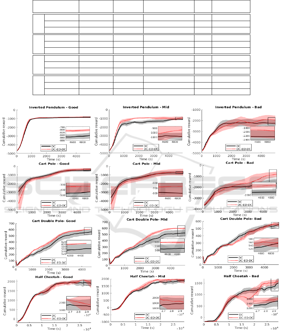
Table 3: Ensemble Strategies Conﬁguration.

strategy

ensemble

aggregation

percentile

ﬁltering

scoring

active set

aggregation

BASE

DC — — — 1.0 data center

DB — — — 1.0 density based

M — — — 1.0 mean

DCR-B — — data center ranking 0.01 best

DS-B — — density scores 0.01 best

M-ED-B mean — euclidean distance 0.01 best

DCR-DC — 25% data center ranking 0.01 data center

DS-DB — 25% density scores 0.01 density based

M-ED-M mean 25% euclidean distance 0.01 mean

M-ED-DC mean 25% euclidean distance 0.01 data center

M-ED-DB mean 25% euclidean distance 0.01 density based

DC-ED-DC data center 25% euclidean distance 0.01 data center

Figure 3: Illustration of DC and DC-ED-DC Learning curves.

In the mid group, cart pole does not present good con-

vergence. The bad group of cart pole presents perfor-

mance compared to mid for the DC-ED-DC strategy.

This environment performs better when policies are

more consistent. The DC-ED-DC strategy presented

the lowest error, Equation (8), having 2.3% average

relative regret. Figure 3 shows an illustration of the

learning curves with strategy DC and DC-ED-DC.

A History-based Framework for Online Continuous Action Ensembles in Deep Reinforcement Learning

585

4.3 Half Cheetah Test

Half cheetah (Todorov et al., 2012) is a complex en-

vironment chosen to validate the strategy of online

continuous action ensembles. It seeks the goal of

a bipedal walk. The half cheetah v2 environment

is tested with DC (best base case strategy) and DC-

ED-DC (best strategy with the lowest error method

as described in the Section 4) for comparison of re-

sults. Table 7 presents the pre-learned and online

learning ensemble strategies’ performance in the half

cheetah environment respectively. The noteworthy re-

sult is that half cheetah learns consistently better for

online learning when compared to the best individ-

ual simulations. Considering the best single parame-

terization in our set, the DC-ED-DC online learning

strategy shows 45% improvement in the good group

(2057±72 vs. 1419±73). Overall, the DC-ED-DC is

consistently better than, or equal (mid group), to the

base case DC. Besides that, training policies online

presents much better results than using pre-learned

policies.

Finally, to test the decreased hyperparameter tun-

ing effort in our approach, random continuous values

of the hyperparameters’ intervals described in Sec-

tion 3 were generated. Note that, due to the random

choice, the chosen parameters naturally tend to fall

more in the middle of the range than at the extremes,

generating more acceptable average values (Table 1).

For a random test, 30 ensembles with 16 parameteri-

zations were generated and run once. In the previous

experiments, the formation for groups always ensured

that at least 4 algorithms (good group) were not able

to converge. In contrast, for the random generation no

such control was made. The random Half Cheetah v2

hyperparameter ensemble using the DC-ED-DC strat-

egy resulted in mean performance of 3684±626.

5 DISCUSSION

In literature, the density-based aggregation strategy

showed better results in the experiments performed

(Wiering and Van Hasselt, 2008; Hans and Udluft,

2010; Duell and Udluft, 2013), although the case

studies analyzed in this article have shown more con-

sistent data center results. One reason may be the

need to parameterize density, which may have nega-

tively inﬂuenced performance. Another consideration

is that both the off-policy algorithm and the environ-

ments are different. Still, there are good results in the

combined strategies of the framework that include the

density algorithm.

Regarding the separation of the tests into groups,

the good group presented better results as expected.

Another point is that the best ensemble strategies in

the good group perform considerably better than the

best individual algorithm, while the density based

strategy performs less consistently. That is, the best

ensemble results improve robustness and accuracy as

expected (Zhang and Ma, 2012). Although the best

strategy varies with group and environment, DC-ED-

DC showed more consistent overall performance.

Looking at the other groups, the mid group for

some cases was able to keep up with the expected

good performance allowing signiﬁcant leeway in

choosing hyperparameter realizations. In the bad

group, the cart double pole and half cheetah environ-

ments surprisingly presented performance compara-

ble to the best tuned run. The former environment

already started in the ﬁnal position equilibrium. The

latter showed the ability to maintain excellent perfor-

mance over the best individual algorithm, mainly be-

cause of the 45% improvement demonstrated in the

good group.

The ﬁnal fully randomized validation test demon-

strated the performance of hyperparameters found

randomly within the composition expected in a real-

istic DDPG implementation. In the half cheetah envi-

ronment, it can be seen that the strategies performed

surprisingly well compared to the single run.

6 CONCLUSION

This article proposed the use of continuous action en-

sembles while learning control policies from scratch.

It demonstrated a reduction in the need for hyperpa-

rameter tuning in DDPG algorithms when testing in

the half cheetah environment. To achieve this we in-

troduced a history-based framework that considers the

ensemble’s historical performance.

The framework proposed is capable of capturing

different compositions of ensemble strategies, pre-

senting a combined ensemble strategy as the one that

performed the best. The best strategy DC-ED-DC,

takes the squared euclidean distance of each action

from the average found by the data center, performs

the moving average by updating the scores, selects

25% of the actions with best scores and applies the

data center algorithm again. This paper made compar-

isons with ensemble strategies presented in the state

of the art and demonstrated that the chosen strategy

outperforms the baseline algorithms. It also demon-

strated the advantage in simulation of using an ensem-

ble algorithm over individual algorithms.

In the benchmark environments, pre-learned

strategies mostly showed better results than online

ICAART 2021 - 13th International Conference on Agents and Artiﬁcial Intelligence

586

Table 4: Pendulum results for different ensemble strategies (31 runs).

strategy

pre-learned learning online learning

good mid bad good mid bad

BASE

DC -779±11* -894±89 -2327±367 -850±25 -1075±80 -2244±321

DB -846±75 -1406±189 -2553±279 -1594±264 -2633±342 -2810±254

M -1416±115 -2851±116 -4043±62 -2835±286 -3574±172 -4234±108

DCR-B -775±10* -874±176 -2388±428 -804±17* -841±59 -2477±413

DS-B -794±22* -1188±325 -3339±206 -1783±343 -2233±376 -3468±79

M-ED-B -1067±353 -1490±509 -3359±518 -810±18 -1358±442 -2343±584

DCR-DC -770±10* -876±180 -2386±430 -791±13* -1008±176 -2341±375

DS-DB -796±33* -1471±398 -3433±135 -846±24 -1105±94 -2346±379

M-ED-M -793±20* -884±63 -2174±486 -894±159 -1139±251 -2369±374

M-ED-DC -778±13* -786±12* -1765±489 -790±11* -783±12* -1677±444

M-ED-DB -782±11* -799±13* -1713±486 -793±10* -861±77 -1448±306

DC-ED-DC -775±11* -864±182 -2066±471 -806±14 -974±201 -1913±400

Table 5: Cart Pole results for different ensemble strategies (31 runs).

strategy

pre-learned learning online learning

good mid bad good mid bad

BASE

DC -392±51* -507±162 -1062±247 -463±170 -783±261 -1684±364

DB -931±138 -1189±144 -1582±183 -1077±206 -1317±279 -1322±214

M -516±109 -878±222 -1637±233 -2153±254 -2805±249 -3411±294

DCR-B -306±54* -571±230 -1180±326 -434±143 -831±319 -1895±435

DS-B -860±148 -1373±173 -2190±240 -920±272 -2020±379 -2316±365

M-ED-B -379±115* -985±326 -2349±542 -379±99* -1382±410 -2483±392

DCR-DC -275±54* -550±220 -1141±313 -727±351 -812±303 -1450±440

DS-DB -380±54* -510±157 -1062±249 -462±164 -735±288 -1338±289

M-ED-M -268±27* -363±160* -924±247 -632±158 -1851±431 -2624±504

M-ED-DC -244±20* -315±144* -1083±418 -296±94* -913±441 -2474±604

M-ED-DB -263±24* -352±157* -953±269 -236±24* -766±377 -1659±531

DC-ED-DC -228±15* -362±170* -837±291 -340±121* -677±367 -912±291

Table 6: Cart Double Pole results for different ensemble strategies (31 runs).

strategy

pre-learned learning online learning

good mid bad good mid bad

BASE

DC 609±10 554±27 485±32 565±42 392±60 551±33

DB 222±62 225±65 183±57 278±61 234±49 296±65

M 535±42 435±45 317±35 88±12 89±11 84±11

DCR-B 603±18 502±42 436±43 612±2 598±12 577±26

DS-B 292±64 258±58 218±53 523±51 368±52 477±48

M-ED-B 577±27 477±51 406±47 552±41 419±52 287±48

DCR-DC 613±3 509±39 435±39 611±2 595±12 560±27

DS-DB 610±7 555±26 499±33 247±31 530±48 462±57

M-ED-M 603±10 546±38 479±40 485±36 292±40 258±29

M-ED-DC 611±3 557±33 494±40 606±7 571±25 467±45

M-ED-DB 606±8 561±29 488±39 606±6 599±10 534±31

DC-ED-DC 614±3* 587±24 500±41 606±5 600±10 560±27

Table 7: Half Cheetah v2 validation results (10 runs).

strategy

pre-learned learning online learning

good mid bad good mid bad

DC 1324±144 1043±249 1002±146 1945±222* 1870±201* 1325±322

DC-ED-DC 1501±39* 817±459 1166±83 2057±72* 1962±229* 1515±174*

A History-based Framework for Online Continuous Action Ensembles in Deep Reinforcement Learning

587

learning. However, evaluating the half cheetah en-

vironment, the approach to online learning policies

made a very signiﬁcant difference. Improving per-

formance for both the base case strategy and the best

strategy, DC-ED-DC. Online learning and the use of

a single environment have advantages in the applica-

bility of the system in real-world robotic applications.

For future work, we would like to test with other

environments. A limitation of this work is that it only

uses the policies’ actions. It would be interesting to

also consider other variables, such as their value func-

tion, as ensemble or incorporating the value functions

into the framework.

REFERENCES

Bertrand, H. (2019). Hyper-parameter optimization in deep

learning and transfer learning: applications to medi-

cal imaging. PhD thesis, Universit

e Paris-Saclay.

Duell, S. and Udluft, S. (2013). Ensembles for continu-

ous actions in reinforcement learning. In ESANN 2013

proceedings, pages 24–26, Bruges, Belgium.

Fernandez, F. C. and Caarls, W. (2018). Parameters tun-

ing and optimization for reinforcement learning al-

gorithms using evolutionary computing. In Interna-

tional Conference on Information Systems and Com-

puter Science (INCISCOS), pages 301––305, Quito,

Equador. IEEE.

Hans, A. and Udluft, S. (2010). Ensembles of neural net-

works for robust reinforcement learning. In 2010

Ninth International Conference on Machine Learning

and Applications, pages 401–406, Washington, USA.

IEEE.

Jaderberg, M., Dalibard, V., Osindero, S., Czarnecki,

W. M., Donahue, J., Razavi, A., Vinyals, O., Green,

T., Dunning, I., Simonyan, K., et al. (2017). Pop-

ulation based training of neural networks. CoRR,

abs/1711.09846.

Jung, W., Park, G., and Sung, Y. (2020). Population-

guided parallel policy search for reinforcement learn-

ing. arXiv preprint arXiv:2001.02907.

Khadka, S., Majumdar, S., Nassar, T., Dwiel, Z., Tumer,

E., Miret, S., Liu, Y., and Tumer, K. (2019). Collab-

orative evolutionary reinforcement learning. In Pro-

ceedings of the 36th International Conference on Ma-

chine Learning, volume 97 of Proceedings of Machine

Learning Research, pages 3341–3350, Long Beach,

California, USA. PMLR.

Krislock, N. and Wolkowicz, H. (2012). Euclidean distance

matrices and applications. In Handbook on Semideﬁ-

nite, Conic and Polynomial Optimization, pages 879–

914. Springer, Boston, MA.

Li, L., Jamieson, K., DeSalvo, G., Rostamizadeh, A., and

Talwalkar, A. (2018). Hyperband: A novel bandit-

based approach to hyperparameter optimization. Jour-

nal of Machine Learning Research, 18(1):6765–6816.

Lillicrap, T. P., Hunt, J. J., Pritzel, A., Heess, N., Erez, T.,

Tassa, Y., Silver, D., and Wierstra, D. (2016). Con-

tinuous control with deep reinforcement learning. In

Proceedings of International Conference on Learning

Representations, San Juan, Puerto Rico.

Liu, R. and Zou, J. (2018). The effects of memory replay in

reinforcement learning. In 56th Annual Allerton Con-

ference on Communication, Control, and Comput-

ing (Allerton), pages 478–485, Monticello, IL, USA.

IEEE.

Mnih, V., Heess, N., Graves, A., et al. (2014). Recurrent

models of visual attention. In Advances in neural in-

formation processing systems.

Silver, D., Lever, G., Heess, N., Degris, T., Wierstra, D., and

Riedmiller, M. (2014). Deterministic policy gradient

algorithms. In Proceedings of the 31st International

Conference on International Conference on Machine

Learning, volume 32, pages 387–395, Bejing, China.

JMLR.org.

Sutton, R. S. and Barto, A. G. (2018). Introduction to Re-

inforcement Learning. MIT Press, Cambridge, MA,

USA.

Tan, J., Zhang, T., Coumans, E., Iscen, A., Bai, Y., Hafner,

D., Bohez, S., and Vanhoucke, V. (2018). Sim-to-

real: Learning agile locomotion for quadruped robots.

arXiv preprint arXiv:1804.10332.

Todorov, E., Erez, T., and Tassa, Y. (2012). Mujoco:

A physics engine for model-based control. In 2012

IEEE/RSJ International Conference on Intelligent

Robots and Systems, pages 5026–5033. IEEE.

Triola, M. F. (2015). Elementary Statistics Technology Up-

date. Pearson Education, Rio de Janeiro, Reprint

(Translated), 11th edition.

Uhlenbeck, G. E. and Ornstein, L. S. (1930). On the theory

of the brownian motion. Physical review, 36(5):823.

Wiering, M. A. and Van Hasselt, H. (2008). Ensemble algo-

rithms in reinforcement learning. IEEE Transactions

on Systems, Man, and Cybernetics, Part B (Cybernet-

ics), 38(4):930–936.

Wistuba, M., Schilling, N., and Schmidt-Thieme, L. (2015).

Sequential model-free hyperparameter tuning. In

2015 IEEE International Conference on Data Mining,

pages 1033–1038.

Wu, J. and Li, H. (2020). Deep ensemble reinforcement

learning with multiple deep deterministic policy gra-

dient algorithm. Mathematical Problems in Engineer-

ing, 6:1–12.

Zhang, C. and Ma, Y. (2012). Ensemble machine learning:

methods and applications. Springer Science & Busi-

ness Media.

ICAART 2021 - 13th International Conference on Agents and Artiﬁcial Intelligence

588