Imperfect Oracles: The Effect of Strategic Information on Stock Markets

Miklos Borsi

Department of Computer Science, University of Bristol, Bristol, U.K.

Keywords:

Economic Agent Models, Multi-Agent Systems, Stock Markets.

Abstract:

Modern ﬁnancial market dynamics warrant detailed analysis due to their signiﬁcant impact on the world. This,

however, often proves intractable; massive numbers of agents, strategies and their change over time in reaction

to each other leads to difﬁculties in both theoretical and simulational approaches. Notable work has been done

on strategy dominance in stock markets with respect to the ratios of agents with certain strategies. Perfect

knowledge of the strategies employed could then put an individual agent at a consistent trading advantage.

This research reports the effects of imperfect oracles on the system - dispensing noisy information about

strategies - information which would normally be hidden from market participants. The effect and achievable

proﬁts of a singular trader with access to an oracle were tested exhaustively with previously unexplored factors

such as changing order schedules. Additionally, the effect of noise on strategic information was traced through

its effect on trader efﬁciency.

1 INTRODUCTION

A line of research was started by Vernon Smith’s ex-

periments in a paper (Smith, 1962) studying the trad-

ing behaviour of humans and allocative efﬁciency of

the market as a whole in a Continuous Double Auc-

tion, the style of market mechanism used in almost all

ﬁnancial exchanges around the world. This work was

groundbreaking for its experimental approach to eco-

nomic theory which previously often held unclear or

inaccurate prior beliefs about its claims. For example,

the number of participating agents in a double auction

that achieves a good equilibrium was deﬁned as “nu-

merous” or with the common mathematical approx-

imation “close to inﬁnite”. In the real, reproducible

situation however, the “invisible hand” of the market

was shown to be in effect from as little as 8 agents, 4

buyers and 4 sellers, who were also untrained for the

situation.

Initial work by Gode and Sunder (Gode and Sun-

der, 1993) indicated that traders with practically zero

intelligence - but some constraints - can produce the

invisible hand effect as well. This was later proven by

Cliff to be a mere byproduct of the underlying proba-

bility distribution and the supply-demand curves used

(Cliff and Bruten, 1997).

Cliff proposed an algorithm called Zero Intel-

ligence Plus that emulated the previous attempt to

https://orcid.org/0000-0002-2185-7404

make a minimally intelligent trading algorithm. In

IBM’s 2001 experiments (Das et al., 2001) algo-

rithmic traders were able to outperform humans and

made 7% more proﬁt on average. The algorithms in-

cluded ZIP, Kaplan’s Sniper and Gjerstad-Dickhaut

(Gjerstad and Dickhaut, 1998) (Tesauro and Bredin,

2002) (Rust et al., 1992) (Rust et al., 1994).

The next addition to the algorithmic roster came in

2008 with Vytelingum’s paper on the Adaptive Ag-

gressive trading strategy (Vytelingum, 2006), which

has been shown to be dominant over human traders in

every scenario.

The introductory study claimed that it is dominant

over the other algorithms previously mentioned but

that claim has not fully held up in subsequent research

by other authors. Different ratios of trading agents

in the market lead to different strategies being dom-

inant. It is not enough to pit two algorithms against

each other in varying ratios and declare a winner if

all pairwise scenarios are one-sided. One must con-

sider the entire trading environment with other traders

and strategies in the background, as well as different

market conditions - changes in supply or demand over

time or a shift in price. See (Snashall and Cliff, 2019)

for a more detailed discussion of when and why AA

does not always dominate.

The simulations discussed in this paper are

based on (Cliff, 2018), available on GitHub at

https://github.com/davecliff/BristolStockExchange.

Borsi, M.

Imperfect Oracles: The Effect of Strategic Information on Stock Markets.

DOI: 10.5220/0010198201970204

In Proceedings of the 13th International Conference on Agents and Artiﬁcial Intelligence (ICAART 2021) - Volume 1, pages 197-204

ISBN: 978-989-758-484-8

197

1.1 An Argument for Strategic Analysis

There is a constant stream of research aimed at dis-

cerning market trends and the effects of various real-

world phenomena on them. While this is a useful pur-

suit in general, there is an argument for taking a dif-

ferent approach to market dynamics.

An intuitive approach to the research hypothe-

sis would be as such: imagine a rock-paper-scissors

game played by thousands. If one particular player

were to know that 60% of the other players always

show rock, said knowledgeable player would adapt

their strategy to show more papers and such on aver-

age win more matches.

Of course, this is an extremely simpliﬁed view.

Stock markets have many more variables, informa-

tion and more complex strategies. These strategies

often adapt to market conditions every second. Yet

still, past research has shown that in certain condi-

tions, certain algorithms are dominant over other al-

gorithms. If one agent was given information about

what algorithms the others were following - but not

their internal variables - could they reliably pick a

dominant algorithm for themselves? And would the

addition of another agent into the trader pool lessen

this dominant algorithm advantage?

The research hypothesis was that if traders were

in possession of perfect strategic information, then

they would be able to signiﬁcantly outperform other

traders not in possession of said information, in a ma-

jority of cases. In addition, this advantage was ex-

pected to decrease once noise is added to the infor-

mation.

The high-level objective of this research project

was to establish an upper bound for proﬁt gained from

strategic information in a market and analyse the loss

in proﬁt from noise in the information. Speciﬁcally,

the aims were:

1. Establish an upper bound for advantage gain-able

from perfect knowledge of the strategies used by

other traders in a stock market.

2. Introduce noise to the strategic information

through a prediction simulation with a distorted

trader strategy ratio.

3. Map the severity of the noise to the loss in advan-

tage.

4. Examine the underlying trader ratio dynamics.

5. Check the effect of different order schedules on

occurring phenomena.

2 EXPERIMENTS

This section will explain the approach taken

to experiment design, focusing on what factors

were accurately measured and what other factors

may inﬂuence the results. All parameters af-

fecting the simulation are shown and discussed,

and the code is available online on GitHub at

https://github.com/borsim/imperfect oracles for easy

reproducibility. As previously mentioned, all possible

combinations of traders have been tried, with some

constraints. Combinations included at least 1 of each

trader type and had an equal number of buyers and

sellers for each strategy. These experiments are novel

in the way that they focus on two previously unex-

plored factors in stock market dynamics: dynamic and

varied supply/demand schedules; and strategic infor-

mation. Neither of these factors was previously indi-

vidually tested in depth and their combination brings

additional interactions to be discussed as well.

2.1 Strategic Information

Strategic information is at the core of the research hy-

pothesis; it was tested exhaustively. Every single pos-

sible combination of the discussed four trading algo-

rithms was simulated for every order schedule. This

ensured a good coverage of all possible scenarios of

strategies in the market. Trader ratios of higher granu-

larity that are not directly mapped out by these experi-

ments may be approximated by interpolating from the

closest ratio points.

2.2 Supply/Demand Schedules

Supply/demand schedules cannot be exhaustively

tested: the number of possibilities is dependent on

multiple potentially inﬁnite variables. To produce

a good coverage of scenarios a randomization ap-

proach was taken. Order schedules were crafted from

a multi-dimensional space. They were composed of

a number of sub-schedules, each with its own set of

parameters. The only constraint was that supply and

demand schedules do not change independently; sub-

schedules on the supply and demand side were re-

spectively equally long in duration. The number of

dimensions in this space varied based on the ﬁrst ran-

domized parameter, the number of sub-schedules.

Simulations were run for a number of timesteps.

Each timestep allowed each trader to act and react

once, issue orders and update internal values. The full

duration was divided into intervals - this controlled

the frequency of customer order replenishment and

change cycles.

ICAART 2021 - 13th International Conference on Agents and Artiﬁcial Intelligence

198

• Drawn once per order schedule:

– Number of sub-schedules (integer)

– Duration of sub-schedules (integer)

– Time mode (set of possible values)

• Drawn once per sub-schedule:

– Volatility (integer)

– Midprice change (integer)

– Step mode (set of possible values)

The full order schedules were crafted with the se-

quence of steps shown in Algorithm 1.

2.2.1 General Experiment Parameters

Simulations were ran for 240 timesteps, split into at

most 8 intervals of 30 steps. These intervals each con-

tained orders arriving to the traders. Orders prices in

this interval averaged 100 ± 40, with each individual

order being at most 60 away from the midprice. The

timing of the orders is set by the deployment function.

The market contained a total of 32, 16 buy-only and

16 sell-only agents. Every possible combination of

traders was tried for 100 random schedules.

• Time Parameters: duration: 240, interval: 30,

maximum number of sub-schedules: 8

• Order Schedule Parameters: midprice: 100,

maximum volatility: 60, maximum midprice

change: 40

• Order Deployment Parameters: stepmode:

ﬁxed/jittered/random, timemode: periodic/drip-

poisson/drip-jittered/drip-ﬁxed

• Trader Parameters: number of buyers: 16, num-

ber of sellers: 16

• Simulation Parameters: number of order sched-

ules: 100, trials for a given trader combination and

given schedule: 1

2.3 Establishing the Baseline

The ﬁrst experiment established a baseline, a clear

limit for the maximum possible efﬁciency/proﬁt

achievable by a trader with access to a perfect ora-

cle providing information about the strategies of other

market participants. See Figure 1 for an overview of

the experiment design.

A “control group” market simulation was per-

formed for a given order schedule and a given com-

bination of traders. The simulation returns the aver-

age proﬁt achieved by traders of particular types. This

serves as the oracle. The trader type with the highest

average proﬁt was deemed “dominant”. There was

Algorithm 1: Creating series of random order sched-

ules.

Draw timemode with even probability from

{periodic, drip − poisson, drip −

jittered, drip − f ixed}

Draw # of sub-schedules with even

probability from {1, 2, ..., max schedules}

for (num intervals -

max schedules) do

Extend an evenly drawn random

sub-schedule’s duration by

interval length

end

supply schedules = {}

demand schedules = {}

for num schedules do

for {supply-side, demand-side} do

Draw volatility with even probability

from {0, 1, ..., max volatility}

Draw midprice change with even

probability from {mid price −

max change, ..., mid price +

max

hange}

Draw stepmode with even probability

from { f ixed, random, jittered}

Set price range lower bound to

mid price + mid price change −

volatility

Set price range upper bound to

mid price + mid price change +

volatility

Set schedule step mode to the

random step mode Set sub-schedule

duration to value calculated before

the loop

end

Append sub-schedule to respective list

end

return order schedule = {timemode,

supply schedules, demand schedules}

no distinction between buyers and sellers for the pur-

poses of strategy dominance, their account balances

were pooled to obtain the average. An additional

trader of this dominant type was added to the buyer

and the seller pool - this was to take into account the

effect of an intelligent agent on the market. Simulat-

ing a market then counting the best outcome will be,

simply put, the best. Simulating a market and slightly

changing the conditions this way will show if the ob-

servations have actionable value and whether some-

thing optimal in one setting could remain close to op-

timal in another.

The second simulation was performed with the

Imperfect Oracles: The Effect of Strategic Information on Stock Markets

199

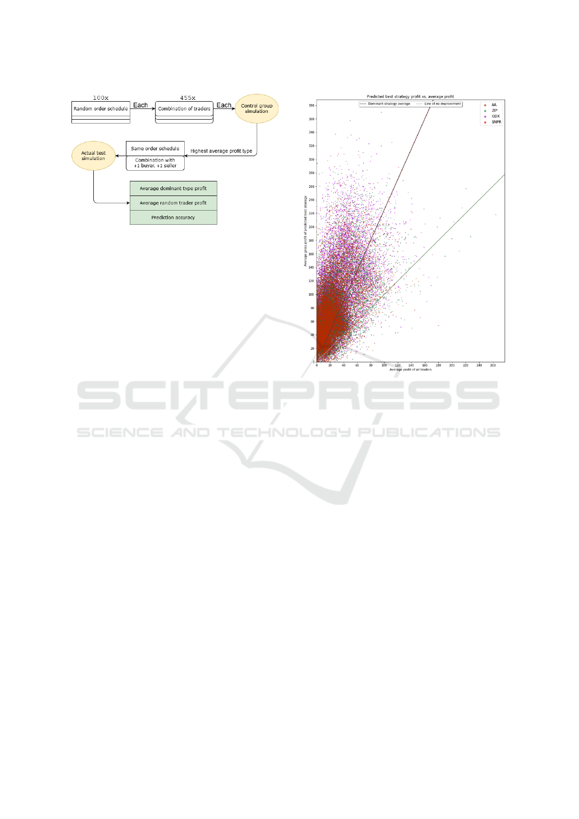
Figure 1: Design of Experiment 1.

thusly expanded pool, this time to obtain the real data.

Between the two simulations trader strategy ratios

and overall supply/demand patterns were shared. Par-

ticular orders may be different if the stepmode con-

tained randomness - i.e. it was not ﬁxed. The se-

quence of order arrivals may also differ.

The expected result of the experiment was that

traders following the optimal strategy determined in

the control simulation would usually dominate in the

repeated simulation. The concrete amount of proﬁt

earned of course depended on the supply/demand

schedule the simulation was performed with. For this

reason the target end result of the experiment was a

ratio; a multiplier on the average trader’s proﬁt.

2.3.1 Results of Experiment 1

The results of Experiment 1 can be viewed in this rep-

resentation on Figure 2. It shows a comparison of how

the strategy predicted as dominant fared in the sec-

ond simulation with the expanded trader pool. The

axes mark the gross average proﬁt per trader of the

predicted dominant type and the colour of points in-

dicates which strategy it is. For added visibility the

“breakeven line” is also plotted - on this line the pre-

dicted best type trader earned exactly as much as the

market average.

The data conﬁrmed the abovementioned expecta-

tions. A number of points fell below the breakeven

line but the majority are above and the data could be

reasonably ﬁt on a line. Predicting the best strategy

would, indeed, on average keep a trader above market

average.

2.4 Experiment 2

Experiment 2 attempted to measure the effect of the

noise described in the experiment design section. A

similar overall design was adopted for Experiment 2.

The signiﬁcant difference was the presence of a dis-

tortion between the prediction and the actual test ra-

Figure 2: Overall results of Experiment 1.

tios. Additionally, the number of order schedules and

trader combinations varied; this was only a numerical

difference and does not have an effect on methodol-

ogy.

Experiment 2 was not immediately conclusive.

Smaller scale trials were run ﬁrst to conﬁrm the pres-

ence (or lack thereof) of correlation before com-

mitting a large amount of computational resources.

Methodology was then adapted to reduce the noise in

the resulting data. Finally a large trial was performed

to provide more accurate numerical output showcas-

ing the merit of the previous changes. All components

of Experiment 2 had the market session duration ex-

tended from 240 to 330 timesteps.

2.4.1 Deﬁnition of Noise Used in this Experiment

One could have selected a different deﬁnition of noise

and it would not inﬂuence the validity of the results

derived here. It is possible to conduct analysis on

different noise patterns by looking purely at the data

points and connecting any two as a prediction and re-

sult into a different noise deﬁnition. The particular

noise function for this research was chosen for sim-

plicity and intuitive ease. It is parametrized by a sin-

gle parameter p. Each trader in the “real” point has p

probability of being viewed as one following a strat-

egy that is not the same as their true strategy. The

ICAART 2021 - 13th International Conference on Agents and Artiﬁcial Intelligence

200

“mistaken” strategy is chosen with an even probabil-

ity from the strategies present in the market, exclud-

ing the “true” strategy. As such p scales the expected

distance of the prediction point from the real point

and the direction was chosen uniformly from the set

of available points. By this deﬁnition maximum noise

was achieved when all traders have an equal probabil-

ity of being seen as any strategy.

max

= 1 − (

|S|

)

where S is the set of possible strategies and |S| denotes

the number of elements in S.

2.4.2 Inconclusive Trial

The ﬁrst trial closely followed Experiment 1. It also

involved 100 random order schedules. Each order

schedule was assigned a noise p with the ﬁrst hav-

ing 0%, the second 0.75% following to the 100th hav-

ing (75 − 0.75)% and each of these schedules had all

trader combinations trialed once. The line ﬁt coefﬁ-

cient was less than 0.0003 away from horizontal and

visual observation did not reveal strong trends that

were covered with noise or outliers. This means that

there was no evidence that in this case the prediction

conferred a valuable piece of information.

The number of incorrect predictions - cases where

the predicted best type did not earn the highest aver-

age proﬁt - was expected to have an upwards slope as

noise in the prediction ratios increased. While it did

have an upwards slope, the data surrounding it was

very noisy and the change itself was fairly small com-

pared to the full set. With a coefﬁcient of 0.01, at the

highest noise level (where on average each trader is

assigned a type through a roll of a 4 sided die) on av-

erage 7.5 more incorrect predictions were made. This

was a change of 1.5% when in the context of a full

set of 455 prediction-result pairs, the change being a

result of going from zero noise to the maximum possi-

ble noise. Combined with the previous result on prof-

its this suggested that these predictions are just not

particularly good. Over half of them were incorrect

from the outset.

2.4.3 Reduced Randomness in Order Schedules

A followup mini-experiment aimed to check whether

the randomisation of order schedules had too much of

an effect on the outcomes of the previous, inconclu-

sive trial. For this experiment the order schedule was

set to a very simple base case reminiscent of those of

Vernon Smith. The supply and demand ranges had

equal limits, prices were allocated at even steps in

these ranges and resupplied to all traders periodically.

Save for the order-trader allocations and the order of

incoming orders from the set everything else was de-

terministic. This schedule was similarly sampled at

10 distinct noise probabilities.

The line’s slope coefﬁcient was −0.001 (per 1%

of probability). While this was an order of magnitude

greater than that of the previous experiment it was still

lacking the expected, slightly more marked decrease.

While the overall number of incorrect predictions was

lower in the very simple and deterministic schedule,

the environment was still noisy and the smaller num-

ber of points in this mini-experiment even produced a

downward trend. Considering how poor the ﬁt was it

should just be regarded as no evidence for a correla-

tion.

2.4.4 Averaged Samples

The next mini-experiment focused on the low predic-

tion accuracy shown so far. It sampled the simple

order schedule at 10 evenly spaced probabilities and

introduced a large change in how predictions were

made. More than one prediction was made each time -

in this case, 10. The predicted best trader was the one

that has the highest average proﬁt in the sum of the 10

predictions combined. The real data trials were done

in a similar fashion; the ﬁnal value for a prediction-

real pair was the average proﬁt in the 10 trials. Note

that each prediction used the same (noisy) trader ratio

combination. Trader ratios were not re-randomized

in-between predictions.

As a result of these changes the range of proﬁts

was much narrower. Because multiple trials were av-

eraged with a simple mean calculation that is linear

in its treatment of outliers, the averaged values were

lower as well when contrasted to the least-squares ﬁt

of the previous dataset. The data was far more com-

pact with a range of just 0.5 − 3 instead of 0 − 10,

indicating signiﬁcantly improved prediction accuracy.

Instead of proﬁt multiplier values of 5 and beyond, no

single averaged-trial went above 2.5. However, the

slope of the proﬁt line was still very close to hori-

zontal with a coefﬁcient of 0.001. Despite that, this

coefﬁcient was objectively a more useful value due to

how the narrower and more regular data range led to a

stronger implication of a cause and effect rather than

random noise.

Prediction accuracy further supports the above ar-

gument. The previous prediction accuracy line ﬁt is

of very poor quality and as such exact metrics like

the residuals of the ﬁt were meaningless in context.

The line ﬁt of this experiment, however, was far bet-

ter. It shows the expected clear upward trend - more

noise in the prediction resulted in more wrong pre-

dictions. This trend was also signiﬁcantly higher in

Imperfect Oracles: The Effect of Strategic Information on Stock Markets

201

impact than the previous existing trends. Going from

277 wrong predictions at no noise to 297 at maximum

noise it nearly tripled the previous prediction error

change with a better ﬁt.

For the large scale simulation repeated predictions

and real trials appeared to be a must.

2.4.5 Large-scale Experiment: Repeated

Predictions & Randomized Schedules

One additional change was made in addition to the

previously discussed ones. Due to its low perfor-

mance and unlikeliness of being the best on its own

merit, SNPR traders were taken out of the pool of pos-

sibilities. This resulted in a number of changes to the

starting parameters of the simulation:

• The total number of participating traders de-

creased with the number of available strategies to

4 ∗ 3 = 12 for the prediction trials and 12 + 2 for

the real trials

• The total number of possible trader combinations

dropped from 455 to 55

• The maximum possible noise probability lowered

to 66.6%

Due to how passive and nonadaptive SNPR traders

have proven to be, this change had an additional bene-

ﬁcial effect. The three advanced algorithms were now

in closer contest with fewer bystanders, meaning that

the proﬁt ratio being measured is closer to 1. Previ-

ously all of them had a fair amount of extra proﬁt just

by taking advantage of bad SNPR trades.

This large trial was done on 10 different and ran-

domized order schedules. In one of the schedules

the randomizer produced an unfavourable schedule,

resulting in few to none trades in most of the trials

and as such the data from that was discarded. The

other schedules were tested at 14 distinct noise prob-

abilities in the range of 0% − 65% with increments

of 5%. Each probability point was tested for all 55

trader combinations and each trader combination had

a set of 50 prediction subtrials and 50 real subtrials.

Before the summaries relating to the main hypoth-

esis of this research are presented, a slight correction

in evaluation methods must be made. Previous, less

exhaustive experiments did not show the phenomena

presented below in an impactful way when plotting

proﬁt so the credibility of using least squares line ﬁts

for them has not changed. For this subsection how-

ever, the least squares ﬁt on its own was no longer

an accurate enough tool. The market average proﬁt

should, under every condition, stay constant. In cases

where a line ﬁt would indicate this not being the case,

the line ﬁt is wrong. The market average does not

change with noise and it was taken from all trader

combinations equally for each probability. The target

of analysis is the difference in slopes between the two

lines of market average and enhanced trader average.

Analysis of cases where the market average was not

ﬂat was problematic - though less so than it appears

due to the comparison being point-wise rather than

line-wise. Still, the least-squares ﬁt in some complex

schedules should be taken with a grain of salt.

The observed phenomena still hinted at being the

closest to ﬁtting on a line. Fits of higher degree poly-

nomials were attempted but the higher-rank coefﬁ-

cients were close to 0. Even after increasing pre-

diction accuracy some outlier removal steps still had

to be taken, especially with the re-inclusion of more

complex order schedules. The data range has a com-

plex structure with traders sometimes earning extraor-

dinarily high proﬁts - outliers on the upper end were

far more common than those on the lower end. Out-

liers were removed with a method common in statis-

tics but with slightly different parameters. Generally,

points outside 1.5 times the inter-quartile range are

considered outliers. For the purposes of not losing

too much important data - it should be noted that even

these outliers awerere a result of 50 + 50 individual

data points - this interquartile range requirement was

loosened. The central range was the interdecile range

(between 10% and 90%). The multiplier for accept-

able points was 1 times this range from the edges.

Figure 3 shows the line ﬁts on all schedules. The

colour of the line indicates how good the line ﬁt is; a

darker colour has closer to 0 residuals. The lightest

colour was set as the maximum residuals out of the 9

line ﬁts.

The majority of trends displayed a clear down-

wards slope, among which were the three closest ﬁts.

One third of the studied order schedules displayed an

upwards slope of moderate uncertainty. These trends

are closely paired with the prediction accuracy graphs

in Figure 4, which shows four lines with a downwards

slope where upwards was the expected direction -

more noise meaning more prediction errors. Three of

those coincided with the upwards proﬁt schedules and

one poor line ﬁt of prediction accuracy had a down-

ward slope on the proﬁt graph.

The overall result of the large-scale experiment

supported the research hypothesis. The majority of

order schedules tested show an above-average proﬁt

earned from good predictions that steadily decreased

over increasing prediction noise in strategic informa-

tion. Figure 5 is a visualization of distribution dif-

ferences in the trial proﬁts. It presents comparisons

through nonparametric Wilcoxon tests of the distribu-

tions involved in the nine order schedules.

ICAART 2021 - 13th International Conference on Agents and Artiﬁcial Intelligence

202

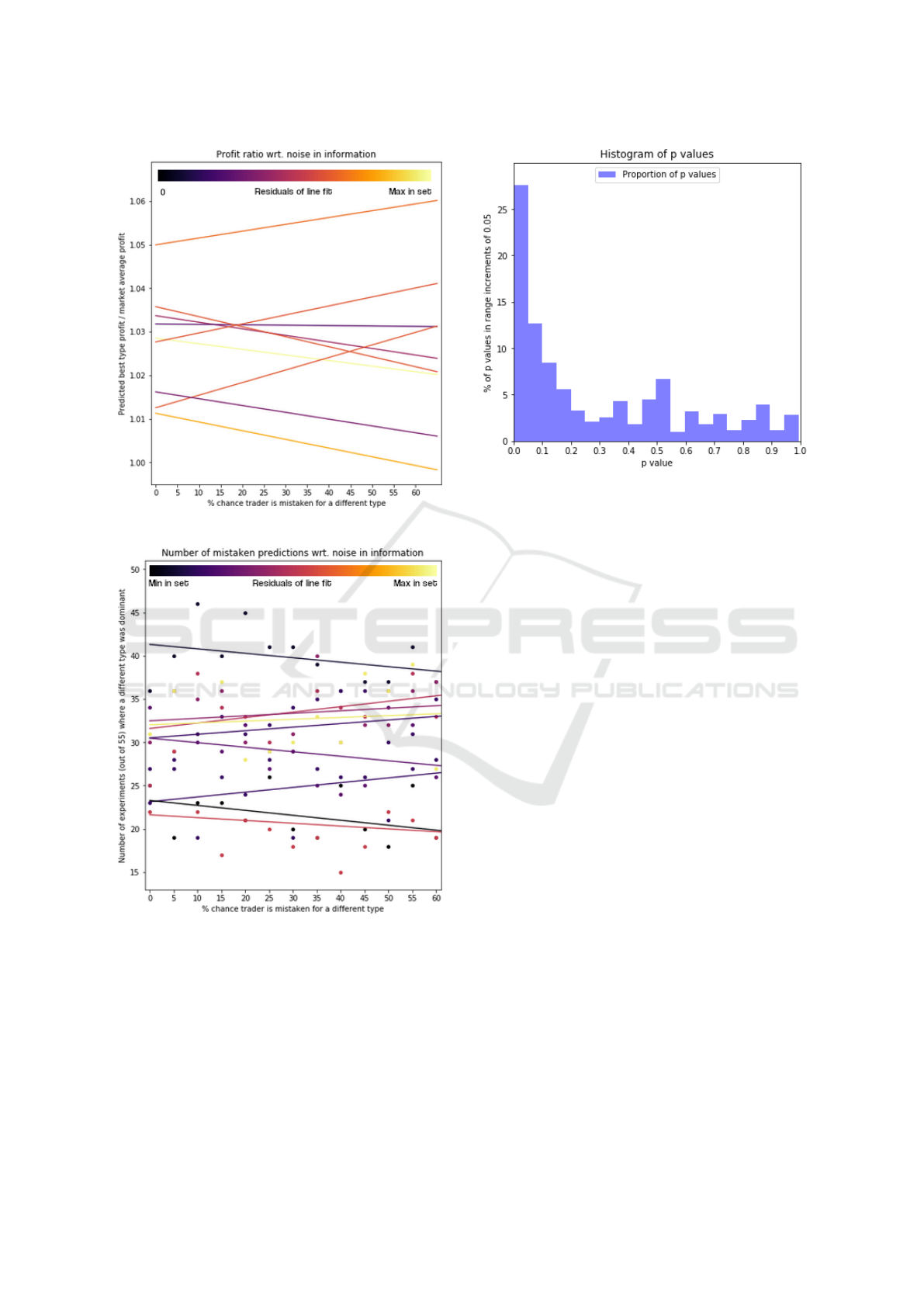
Figure 3: Proﬁt trends for 9 order schedules.

Figure 4: Prediction accuracy for 9 order schedules.

Individual data points are a pairwise comparison be-

tween the noiseless prediction-result distribution and

a noisy prediction-result distribution. Small p values

indicate strong certainty that the samples were drawn

from different distributions. A large portion of these

tests indicate that the samples with noise involved can

usually be distinguished from samples without pre-

diction noise. A possible explanation for the uncer-

tain predictions and upwards proﬁt trends could be

Figure 5: P values of Wilcoxon tests.

that certain order schedules spawned more compli-

cated strategic dynamics. For the majority of sched-

ules the addition of two extra traders of a kind did

not nullify the advantage of having had access to pre-

dictions. However, for the schedules that show nega-

tive correlations, this alteration in trader ratios might

have ended up working against the traders with access

to an oracle, pushing them over the boundary where

the predicted strategy was no longer the optimal one.

Such a scenario could have arisen when most of the

strategic landscape was dominated by a single trader

with very small pockets of other types. Figure 6 and

Figure 7 show a comparison between Schedule 3 -

where predictions performed well - and Schedule 7

where they did not.

3 CONCLUSIONS

The fairness and regulatory tools of ﬁnancial mar-

kets draw notable attention, especially after reces-

sions like the 2008 housing crash or the fallout of the

2020 COVID pandemic. It is vital to have scientiﬁ-

cally estimated bounds for what advantage is reason-

able as a function of access to information. This ex-

ploratory study suggests an approximate 10% proﬁt

advantage difference between perfect and no informa-

tion in most cases. Excessive advantage could prove

to be a strong hint towards requiring further, manual

investigation of a market participant.

As well as conﬁrming the initial hypothesis, this

research explored the most signiﬁcant factors inﬂu-

encing market predictions in a simulated environ-

ment. Future research now has a proven process to use

Imperfect Oracles: The Effect of Strategic Information on Stock Markets

203

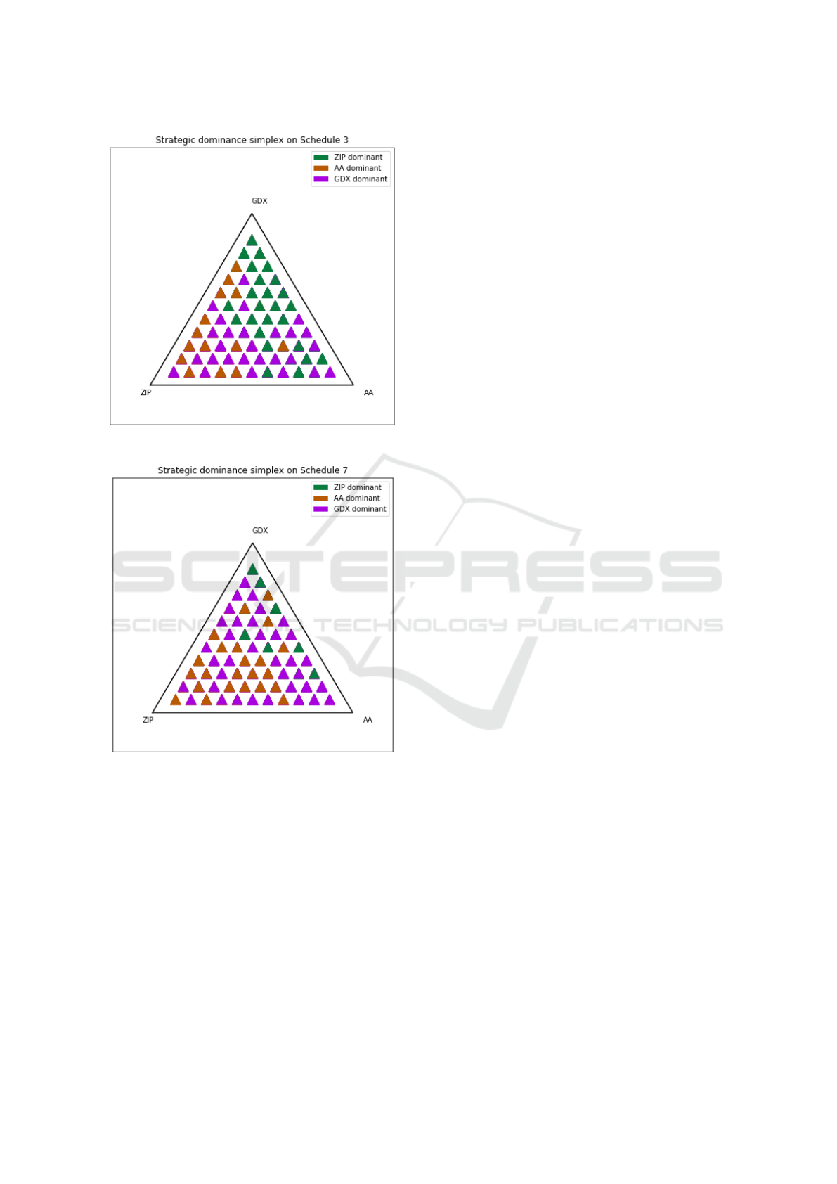
Figure 6: Well-predictable order schedule.

Figure 7: Badly-predictable order schedule.

as a basis, with knowledge of the primary obstacles in

assessing predictions, such as the need for an aver-

age prediction set, as opposed to perfect knowledge

of the current market state. Some failure cases of the

proposed prediction system were also unveiled, where

a counter-intuitive correlation was present. The fail-

ure cases were supported in evidence of their differing

nature from two independent sources of experiment

data, proﬁt ratio and prediction accuracy. Follow-

ing work can either avoid said failure cases or delve

deeper into why they produce the results in question.

This project extended the Bristol Stock Exchange

simulator with more functionality. These extensions

are open for anyone to copy, use or modify. The data

pipeline of the analysis is also published online and

may be used directly on any experiment data ﬁle with

no additional steps.

All data points in the data ﬁles may be reinter-

preted in their relation to each other. The data ob-

tained remains useful as one may perform an analysis

of a different noise phenomenon without the need to

re-generate hundreds of thousands of lines of data.

REFERENCES

Cliff, D. (2018). Bse: A minimal simulation of a limit-

order-book stock exchange. In Affenzeller, M., Bruz-

zone, A., Jimenez, E., Longo, F., Merkuryev, Y., and

Piera, M., editors, 30th European Modeling and Simu-

lation Symposium (EMSS 2018), pages 194–203, Italy.

DIME University of Genoa.

Cliff, D. and Bruten, J. (1997). Zero is not enough: On the

lower limit of agent intelligence for continuous double

auction markets.

Das, R., Hanson, J. E., Kephart, J. O., and Tesauro, G.

(2001). Agent-human interactions in the continuous

double auction. In International joint conference on

artiﬁcial intelligence, volume 17, pages 1169–1178.

Lawrence Erlbaum Associates Ltd.

Gjerstad, S. and Dickhaut, J. (1998). Price formation in

double auctions. Games and Economic Behavior,

22(1):1 – 29.

Gode, D. K. and Sunder, S. (1993). Allocative efﬁciency

of markets with zero-intelligence traders: Market as a

partial substitute for individual rationality. Journal of

Political Economy, 101(1):119–137.

Rust, J., Miller, J., and Palmer, R. (1992). The Double

Auction Market: Institutions, Theories, and Evidence,

chapter Behavior of trading automata in a computer-

ized double auction market. Addison-Wesley, Red-

wood City, CA.

Rust, J., Miller, J. H., and Palmer, R. (1994). Characterizing

effective trading strategies: Insights from a computer-

ized double auction tournament. Journal of Economic

Dynamics and Control, 18(1):61 – 96. Special Issue

on Computer Science and Economics.

Smith, V. L. (1962). An experimental study of competi-

tive market behavior. Journal of political economy,

70(2):111–137.

Snashall, D. and Cliff, D. (2019). Adaptive-aggressive

traders don’t dominate. In ICAART.

Tesauro, G. and Bredin, J. L. (2002). Strategic sequential

bidding in auctions using dynamic programming. In

Proceedings of the First International Joint Confer-

ence on Autonomous Agents and Multiagent Systems:

Part 2, AAMAS ’02, page 591–598, New York, NY,

USA. Association for Computing Machinery.

Vytelingum, P. (2006). The Structure and Behaviour of the

Continuous Double Auction. PhD thesis, University

of Southampton.

ICAART 2021 - 13th International Conference on Agents and Artiﬁcial Intelligence

204